INSTRUMENTAL VARIABLES ESTIMATION WITH
MIXED DATA SAMPLING (MIDAS)
Stephen Goldberger
A dissertation submitted to the faculty of the University of North Carolina at Chapel Hill in partial fulfillment of the requirements for the degree of Doctor of Philosophy in the Department of Economics.
Chapel Hill 2013
Approved by:
Dr. Eric Ghysels
Dr. Saraswata Chaudhuri
Dr. Neville Francis
Dr. David Guilkey
c
2013
Stephen Goldberger ALL RIGHTS RESERVED
Abstract
STEPHEN GOLDBERGER: INSTRUMENTAL VARIABLES ESTIMATION WITH MIXED DATA SAMPLING (MIDAS).
(Under the direction of Dr. Eric Ghysels.)
In most discrete time series models, the instrumental variables (IV) of estimation are the
same time frequency as the error term. This is the case even if the underlying theoretical
model allows instruments of a higher time frequency. This dissertation shows the asymptotic
variance of IV parameter estimates may improve when instruments of a higher time frequency
than the error term are utilized. In particular this dissertation shows improvements within the
Mixed Data Sampling (MIDAS) framework for dealing with data series of mixed frequencies.
The estimates improve in terms of asymptotic variance under three separate series of
as-sumptions and methodologies for incorporating higher frequency instruments. First, a general
methodology is outlined for constructing asymptotically better instruments for martingale
dif-ference sequence errors. Second, an argument is made for using MIDAS forecasts to construct
the asymptotically optimal instruments for these martingale difference sequence errors. Finally
for the the assumption of moving average errors being conditionally zero given the information
set, mixed frequency information instruments lead to improvements in parameter estimates.
In addition to mixed frequency instruments, considering mixed frequency moment conditions
also improves estimation. In all three cases, the proposed methods are illustrated on asset
Acknowledgments
I am grateful for all the help and guidance I’ve received over the past 5 years in crafting this
dissertation. I am thankful for the help of my advisor Dr. Eric Ghysels and the members of
my committee: Dr. Saraswata Chaudhuri, Dr. David Guilkey, Dr. Neville Francis, and Dr.
Jonathan Hill. Additionally I’d like to thank all the professors and students I’ve met over the
last 5 years at UNC, who have consistently helped to push the bounds of my understanding
of Economics. Lastly I’d like to thank my beloved wife Dr. Burcu Aydin and my parents for
all their support.
Table of Contents
Abstract . . . iv
List of Tables . . . viii
List of Figures. . . ix
1 Introduction . . . 1
1.1 Motivation . . . 1
1.2 Organization . . . 3
1.3 Background and Related Work . . . 4
2 MIDAS Instruments for More than One Parameter . . . 6
2.1 Motivation . . . 6
2.2 Methodology . . . 8
2.3 Empirical Results . . . 12
2.3.1 Term Structure: Cox-Ingersoll-Ross . . . 13
2.3.2 Integrated Volatility . . . 17
2.4 Conclusion . . . 24
3 Optimal MIDAS Instruments for MDS Errors . . . 25
3.1 Motivation . . . 25
3.2 Affine SDFs and Optimal Instruments . . . 28
3.2.1 Model and GMM Estimation . . . 29
3.2.3 Pseudo-Higher Frequency Test Assets . . . 37
3.3 Methodology . . . 40
3.3.1 Quarterly Horizon Test Assets . . . 41
3.3.2 Psuedo-Higher Frequency Test Assets . . . 44
3.4 Empirical Results . . . 45
3.5 Conclusion . . . 52
3.6 Tables of Results . . . 54
4 Optimal MIDAS Instruments for Moving Average Errors . . . 65
4.1 Motivation . . . 65
4.2 Model and GMM Estimation . . . 66
4.3 Mixed Frequency Information Sets . . . 71
4.4 Methodology . . . 74
4.4.1 Low Frequency Moment condition . . . 75
4.4.2 Mixed Frequency Moment condition . . . 78
4.5 Empirical Results . . . 79
4.6 Conclusion . . . 91
4.7 Tables of Results . . . 92
5 Conclusion . . . 100
A Appendix . . . 101
A.1 Daily Data Time Series from Chapters 3 and 4 . . . 101
A.2 Proof that High Frequency Noncentrality Parameter is Larger . . . 104
A.3 Construction of Σt and Σt . . . 106
A.4 Construction of Risk Free Moment Condition . . . 108
Bibliography . . . 111
List of Tables
2.1 Cox Ingersoll Ross Results . . . 15
2.2 Integrated Volatility Results: Euro . . . 21
2.3 Integrated Volatility Results: Yen . . . 22
3.1 Fixed Instruments . . . 54
3.2 Optimal for Market Portfolio . . . 55
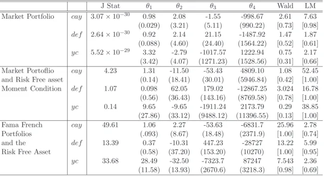
3.3 Optimal for Market, Augmented by Risk Free Moment . . . 56
3.4 Optimal for Market Portfolio and Risk Free Asset. . . 57
3.5 Optimal for 4 Fama French Portfolios, Augmented by Risk Free Moment . . . . 58
3.6 Optimal for 4 Fama French and Risk Free Asset. . . 59
3.7 Fixed Instruments for Low Frequency and Pseudo-higher Frequency Returns . 60 3.8 Optimal for Market and Pseudo-Higher Frequency Market . . . 61
3.9 Optimal for Market, Pseudo-higher Frequency Market, and Risk Free Asset . . 62
3.10 Optimal for Fama French and Pseudo-higher Frequency Fama French. . . 63
3.11 Optimal for Fama French, Pseudo-higher Frequency and Risk Free Asset . . . . 64
4.1 Fixed Instruments . . . 92
4.2 Optimal for Jtlag Low Frequency Moment Condition . . . 93
4.3 Optimal for Jtlag and Mixed Frequency Moment Condition . . . 94
4.4 Mean Square Forecast Error . . . 95
4.5 Optimal for Jt∞ and Low Frequency Moment Condition: Almon . . . 96
4.6 Optimal for Jt∞ and Low Frequency Moment Condition: Beta . . . 97
4.7 Optimal for Jt∞ and Mixed Frequency Moment Condition: Almon . . . 98
A.1 Daily Data Time Series by Name and Classification . . . 101
List of Figures
2.1 MIDAS 1 Weights . . . 15
2.2 MIDAS 2 Weights . . . 16
2.3 Daily Integrated Volatility Euro. . . 21
2.4 Daily Integrated Volatility Yen . . . 22
2.5 MIDAS Weights Euro . . . 23
2.6 MIDAS Weights Yen . . . 23
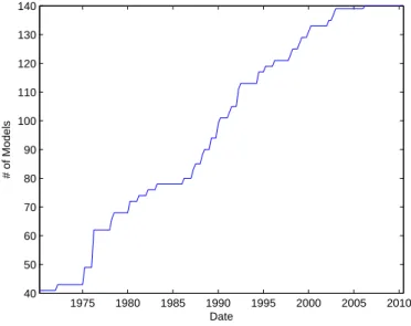
3.1 Number of Models used for Forecast Combinations . . . 48
3.2 Weights for forecast of Et[Rt+1] by Daily Time Series classification . . . 48
3.3 Number of models used in forecast by Daily Time Series classification . . . 49
3.4 Average weight within each Time Series classification in forecast ofEt[Rt+1] . . 50
4.1 Autocorrelations without Restriction, Low Frequency Moment Condition . . . 84
4.2 Autocorrelations with Restriction, Low Frequency Moment Condition . . . 84
4.3 Autocorrelations without Restriction, Mixed Frequency Moment Condition . . 85
Chapter 1
Introduction
1.1 Motivation
Consider a vector time series Yt=1,..t∗ for a fixed time frequency 4t. Suppose in a given
theoretical model, there exists a vector h(θ, Yt=1,..t∗), a function of a K×1 parameter vector
θ as well as the data up to and including time t∗. Furthermore, there exists a θ0, the true
value of the parameters, such thatE[h(θ0, Yt=1,..t+1)|σ(Yt, Yt−1, ...)] = 0. The error vectort
is defined at the true value θ0:
t≡h(θ0, Yτ=1,..t) (1.1)
From repeated application of the law of iterated expectations, the theoretical model
equiv-alently saysEt[t+i] = 0,i≥1. In other words, the model states that {t+i}i≥1 is a martingale
difference sequence with respect to σ(Yt, ...), the natural filtration with respect to the data
series Yt.
Now consider any subset Zt∈σ(Yt, Yt−1, ...). Consider any specificzt∗ ∈Zt and apply the
Law of Iterated Expectations:
E[zt∗t+1] = E[Et[zt∗t+1]]
= E[ztEt[t+1]
= 0
where z∗t is the instrument of choice as a specific case of Generalized Method of Moments
(GMM) as outlined inHansen(1982). The GMM optimal weighting matrix is used to estimate
the true parameter θ0. Instrumental variables can be used as long as the GMM regularity
conditions are satisfied and there are at least an M number of instruments in the set Zt such
thatM ≥K. In other words, one can estimateθ0as long as the model is just or over-identified.
With this framework in place, the question then becomes: Which instruments should one use
to estimate θ0?
Just choosing any and all instruments available can result in a large number of moment
con-ditions which can cause problems as seen inHan and Phillips(2006) andKoenker and Machado
(1999) among others. Under certain regularity conditions in GMM estimation, the parameter
values are consistently estimated no matter which instruments are chosen. It seems natural
that the instruments that yield the most efficient estimates for parameters, or the instruments
which yield the smallest asymptotic variance for the parameter estimates should be chosen.
In the case of just identification, where K=M, and the total number of instruments inZt is
M, the optimal instruments are trivially the only instruments chosen with the optimal
weight-ing matrix for GMM estimation (See Anatolyev (2007)). However, in almost all econometric
specifications for this framework, there will be over-identification.
The choice of optimal instruments in instrumental variables estimation for a time series
Yt=1,...,T with a martingale difference sequence (MDS) has been explored in many earlier
pa-pers. InHayashi and Sims(1983), an optimal IV-estimator utilizing forward-filtering is defined
for a specific model in which instruments are not explicitly exogenous and serial correlation is
allowed in the error term. Hansen and Singelton(1996) define optimal instruments for Linear
Asset Pricing Models (LAPM’s) with moving average errors. Nagel and Singleton(2011) find
optimal instruments for Conditional Asset Pricing Models in the case where there is a
Stochas-tic Discount Factor as an affine function of factors. In the simple case whereyt=x0tβ+tand
E[t+1 |σ(Zt,Zt−1...)] = 0,Chamberlain (1987) finds an explicit form for the optimal
instru-ments when there is no serial correlation in t. In the case of serial correlation, a much more
complicated form for the optimal instrument is required depending on the nature of the
explicit examples and defining their optimal instruments given assumptions like conditional
heteroscedasticity and homoscedasticity. For the earlier assumption that {t+i}i≥1 is a
mar-tingale difference sequence the optimal instrument asymptotically is known fromChamberlain
(1987). This instrument is problematic in application however, since it is not observable and
assumptions regarding the conditional variance of the error are required for its construction.
Consider a second time series YtHF−i N
of a higher frequency thanYt. The index i indicates
the higher frequency observation counting back from time t. Suppose the underlying model
allows the further assumption that E[t+1|σ(Yt, YtHF−I N
, Yt−1, YtHF−1−I N
, ...)] = 0. Then any high
frequency subset ZHF t−i
N ∈
σ(Yt, YtHF−I N
, ...) is a valid instrument for estimation as well.
Addi-tionally, any function of both the low and high frequency instrument sets, F(Zt, ZtHF−i N
), is
a valid instrument as well. This additional information creates a new, stronger restriction
on parameter estimation. This dissertation will explore how this stronger assumption can be
used for estimation of models with martingale difference sequence errors to improve parameter
estimates.
1.2 Organization
This dissertation considers two possible methodologies for utilizing higher frequency
instru-ments to improve the estimation of parameters in terms of the asymptotic standard errors.
In Chapter 2, a very general methodology is outlined, where no assumptions on the second
moments of the errors are made beyond the GMM regularity condition that the variance is
finite. This methodology is designed for higher frequency instruments which give smaller
asymptotic variance by construction. The instruments are chosen from the set of instruments
with smallest estimated asymptotic variance from the data. The method is tested by
con-sidering the Cox, Ingersoll, and Ross (1985) model for the short term interest rate and the
Bollerslev and Zhou (2002) model for integrated volatility.
In Chapter 3, the optimal instruments from Chamberlain (1987) for an MDS error
se-quence is constructed using mixed frequency data. In particular they are applied to the
affine stochastic discount factor asset pricing model from Nagel and Singleton (2011). The
optimal instruments for this asset pricing model are known, but they consist of the
prod-uct of two conditional moments. Chapter 3 proposes the MIDAS forecasting method from
Andreou, Ghysels, and Kourtellos (2010) to be used to construct these conditional moments
using mixed frequency data. The results from estimating according to these MIDAS
opti-mal instruments are compared to the original results from Nagel and Singleton (2011).
Im-provements with regard to the asymptotic standard errors are found. In addition to mixed
frequency instruments, mixed frequency moment conditions or error terms are considered for
estimation as well. In other words the error terms are a function of low and high frequency
data: t≡h(θ0, Yt=1,..t, YtHF=1,..t).
Mixed frequency data leads one to consider errors of different forecast horizons beyond
the next low frequency period. Chapter 4 considers the instruments in situations where the
following moment condition holds: E[t+m|σ(Yt, YtHF, Yt−1, YtHF−1, ...)] = 0 form >1. Errors of
this form are moving average errors of order M−1. The optimal instruments for these errors
are not the same as for an MDS since the autocorrelation must be accounted for. Chapter 4
proposes the IV estimation of this model and construction of the optimal instruments for a
mixed frequency information set. The methodology is then applied to the constant relative
risk aversion linear asset pricing model ofHansen and Singelton (1996).
These three distinct methodologies all entail mixing the frequencies of the data available to
the econometrician. Furthermore, they utilize the MIDAS (Mixed Data Sampling) framework
developed in Ghysels, Santa-Clara, and Valkanov (2005), Andreou, Ghysels, and Kourtellos
(2010a), Ghysels(2012) and other papers.
1.3 Background and Related Work
Mixed Data Sampling or MIDAS refers to the regression models and filtering methods
de-veloped by Ghysels et al with regard to data sampled at different frequencies. Work
deal-ing with this form of regression modeldeal-ing includeGhysels, Santa-Clara, and Valkanov (2005),
Ghysels, Sinko, and Valkanov (2007), andAndreou, Ghysels, and Kourtellos (2010a). In
use of daily financial time series to forecast quarterly and monthly macroeconomic variables,
which is of particular interest to this dissertation. Ghysels and Wright (2010) deals with
MI-DAS instruments and the first chapter of this dissertation is primarily concerned with
improv-ing their methodology by extendimprov-ing it to IV-models with a vector of parameters as opposed
to a scalar. For IV estimation of a scalar, Ghysels and Wright (2010) designed a device for
reducing the dimensionality of instruments in a time series context by using a lag
polyno-mial function of basic instruments. In particular if instruments of a higher frequency are
considered in the lag polynomial there are improvements in small sample performance. The
device involves iterating between solving for the GMM estimate for a particular parameterized
lag polynomial, and solving for the parameterized lag polynomial that leads to the smallest
asymptotic variance for that GMM estimate.
Optimal instrument research with regard to time series models is detailed in Anatolyev
(2007). This dissertation is particularly interested in the optimal instruments ofChamberlain
(1987) from that survey for a martingale difference sequence. The instrument is the conditional
score multiplied by the inverse of the conditional variance of the error. Nagel and Singleton
(2011) considers application of that optimal instrument to an asset pricing model with an
affine stochastic discount factor. The conditional score and variance are estimated using
local-ized polynomial regressions and improvements are found from considering the corresponding
optimal instruments.
Hansen and Singelton (1996) discusses the optimal instruments for errors of a longer
fore-cast horizon. Form >1, an error termt+mwill exhibit autocorrelation, namely the errors will
be moving average errors of order m−1. Hansen and Singelton (1996) discusses the optimal
instruments for linear models at this greater forecast horizon. The paper finds improvements
in small sample estimation from using the instruments.
Chapter 2
MIDAS Instruments for More than One Parameter
2.1 Motivation
Let Yt=1,..t∗ be a vector time series for a fixed time frequency 4t. There is an MDS error
vector t defined at the trueK dimensional parameter value θ0:
t ≡ h(θ0, Yτ=1,..t) (2.1)
E[h(θ0, Yτ=1,..t+1)|σ(Yt, Yt−1, ...)] = 0 (2.2)
For some subset of instrumentsZt∈ σ(Yt, Yt−1, ...), θ0 can be estimated according to
instru-mental variables from the moment conditionE[ztt+1] = 0. This chapter designs a very general
methodology which is applicable to any and all time series models which assume errors which
are martingale difference sequences with respect to a filtration. The method is feasible for
any and all econometric models for which one can acquire higher frequency data points for
Yt and assume the error is conditionally zero for said data points. The proposed instruments
will lead to smaller estimated asymptotic standard errors. This is accomplished by extending
Ghysels and Wright (2010) and developing a MIDAS instrument procedure for the situation
in which the number of parameters K can be greater than 1.
The assumption that the error is a martingale difference sequence is a powerful one: Given
all the information contained in{Zt−i}(i≥0), the instrument subset ofσ(Yt, ...), the expectation
for the error is zero. Suppose the time frequency is one month and zA
t ∈ Zt is the price of
asset A. The data containszA
t ,∀t, and att∗, the model says that the expectation oft∗
not just given the price of asset A at the beginning of month t∗, but given the entire price
history of A up to the beginning of montht∗. Suppose the value ofzA t−i
r
for anyt∈ {1,2, ..t∗},
andi∈ {0,1,2, ..., r} is such thatzAt−i r ∈
Zt∗. Namely, previous higher frequency observations
of instruments are contained in the given instrument set Zt. This means that they are valid
instruments for estimation, since it is assumed thatE[t+1|ztA∗−i r
] = 0.
When estimating the parameters according to Instrumental Variables, one should choose
instruments containing as much of the information as feasible about the current state of the
world, or the conditioning information set Ft =σ(Yt, ...). In particular, instead of just using
data realized at timet, one could use the entire history of data between timetand t−1. The
simplest way to do this would be to use{zA t−i
r}
, i∈ {0, ..., r} as an instrument for estimation.
However if each of the high frequency instruments are stacked into a vector zt, it can be
difficult to invert the matrix ˆS = ˆE[(zt⊗t+1)(zt⊗t+1)0] used in optimal GMM estimation
due to its size. Also inverting may be especially difficult if the data is at a very high frequency
and zA t−i
r
and zA t−i+1
r
are quite similar for all t and i, meaning the matrix may be less than
full rank or ill-behaved in practice. In order to avoid this problem, a solution used in MIDAS
regressions discussed inGhysels, Sinko, and Valkanov(2007) is adopted to this case. In MIDAS
regressions, instead of running a regression on each of thezA t−i
r
data points, a weighted average
of the r observationszA t−i
r
betweent andt−1 is used. In this chapter, a weighted sum of the
instrumentszA t−i
r
are constructed to create a single, new instrument for instrumental variables
estimation. This process for the case where the vectorθ0is a one dimensional scalar is outlined
inGhysels and Wright(2010). That procedure will be adapted for the case whereθ0is aK×1
dimensional vector, K≥1.
Replacing the naive higher frequency instrument specification with a single MIDAS
instru-ment reduces the chosen instruinstru-ment set significantly, allowing for ease in estimation as fewer
moments need to be matched while still ensuring that the restriction that the error be
orthog-onal to the higher frequency previous instruments is not lost. There is a trade off between
using many instruments and ease of estimation. This procedure aims to minimize that trade
off, and reduce the loss of information that comes with reducing the set of instruments used
in estimation.
2.2 Methodology
As in Ghysels and Wright (2010), consider the moment condition Et[h(θ0, Yi=1,...,t+1)] = 0
where{Yt}Tt=1 is a time series, but unlike in Ghysels and Wright letθbe aK×1,K ≥1 vector
of parameters where θ0 is its true value, and h(θ, Yt) is a vector function (possibly scalar).
Recall that t=h(θ0, Yi=1,...,t) in other words a functionh(·) evaluated at the true valueθ0.
Let ∆tbe the initial sampling frequency (i.e., a month, day, quarter, etc) and the number of
higher frequency observations contained within ∆tto ber(i.e. r≈20 daily observations for
ev-ery month). Considerz∗t, one possible higher frequency instrument such that the data includes
observations {zt∗−0 r
, zt∗−1 r
, ...,}. A weighted sum of ther+ 1 instruments{zt∗−0 r
, z∗t−1 r
, ..., zt∗−r r} parameterized by a vector α(i) is constructed. This parameter vector is indexed by i, the ith
moment condition of theM dimensional moment vector. LetDbe the number of instruments
chosen for estimation. Because θ is K ×1, if the dimension of the error vector is C ≥ 1,
C·D≥M ≥K in order to estimateθ0. It is not necessary that allD instruments be MIDAS
instruments, only at least one in order to follow this methodology. In other words, replace
each of the moments for the element c of the error vector t:
E
zt∗
−0rhc,t+1(θ, Yt)
zt∗
−1rhc,t+1(θ, Yt)
.
.
.
zt∗−r
rhc,t+1(θ, Yt)
with a single moment:
E r X j=0
wj(α(i))Ljzt∗
hc,t+1(θ, Yt)
where L is the lag operator operating at smaller sampling frequency 1r. Call the
Pr
j=0wj(α(i)) = 1, however in many applications it may make sense to do so.
The potential weighting schemes are numerous. The weighting scheme to use is based on
matters of convenience, theory and observation. For example, volatility over a trading day has
been found empirically to be smile shaped as there are more trades and price movements at
the beginning and end of the trading day. A smile shaped weighting scheme over the previous
day’s price process for an asset might grant a superior instrument. Two possible weighting
schemes will be introduced below.
One possible weighting scheme is a normalized exponential Almon lag polynomial. Either
in the unrestricted: wu
j or restricted: wrj forms below.
wuj = wj(α1, α2)
wuj = e
α1j+α2j2
Pr
m=0eα1m+α2m
2
wrj = wj(α1,0)
Depending on the magnitude of α1 and α2, the unrestricted weighting scheme is upward,
downward, or smile shaped weighting over the size of the lag. For the restricted model,α1 >0
indicates upward weighting (more weight on older observations) and α1 < 0 is downward. If
α1 = 0 there is equal weighting, or a simple average.
A second weighting scheme utilized is the normalized beta probability density function.
Define xj ≡ ((rj−−1)1)2. Consider the following specifications, unrestricted or restricted, zero or
nonzero weighting on the previous lag:
wu,nzj = wj(α1, α2, α3)
wu,nzj = x
α1−1
j (1−xj)α2−1
Pr m=1x
α1−1
m (1−xm)α2−1
+α3
wr,nzj = wj(1, α2, α3)
wju,z = wj(α1, α2,0)
wjr,z = wj(1, α2,0)
Once an appropriate parameterized weighting scheme wj(α(i))j={0,...,r} and higher
fre-quency data series of interest z∗t are chosen, define:
Ljz∗t ≡ z∗t
−jr (2.3)
b(α(i), L) ≡ r
X
j=0
wj(α(i))Lj (2.4)
fi ≡ b(α(i), L)zt∗ hc(θ, Yt) (2.5)
Thus fi is an element of the moment vector f(Yt, θ, α), constructed with a MIDAS
in-strument. It follows from the earlier extension of the law of iterated expectations that
E[fi(Yt, θ0, α(i))] = 0 for any possible value of α(i). This serves as one moment condition.
Since the vectorθ isK dimensional, only one of the M ≥K moments required for estimation
has been chosen. It is possible to either continue this process to define more MIDAS
instru-ment moinstru-ment conditions or choose another instruinstru-ment to get the proper number of moinstru-ment
conditions needed for estimation.
The M moment conditions are then assembled into a vector f(Yt, θ, α) where at least one
of the conditions is MIDAS-IV as defined earlier. The vectorα consists of the parametersα(i)
which are components of the various MIDAS instruments used to assemble the M moments.
Hence it could contain elements of different dimensions, i.e. α(i) could be an element of R2
and α(j) could be an element of R4.
Note that depending on the specification, if C ≥2, one may decide not to use the same
MIDAS instrument for each of the C elements of the error vector. For example, one may
choose the samezt∗for each of the elements of the error vector, but allow for different weighting
schemes. Alternatively, one can choose completely different z∗t and z∗∗t depending on which
element of the error vector is being multiplied by the instrument. This provides some more
flexibility in estimation.
0, the GMM estimator fromHansen (1982) can be defined as follows for all values of α:
b
θ(α) ≡ arg min
θ
1
T T
X
t=1
f(Yt, θ, α)0W f(Yt, θ, α) (2.6)
where W is the GMM weighting matrix. W is selected to be the optimal weighting matrix
according to continuously updating GMM estimation fromHansen, Heaton, and Yaron(1996),
namely Ω(b θ, α)−1 whereΩ(b θ, α) is a consistent estimate of Ω(θ, α) =E[f(Yt, θ, α)f(Yt, θ, α)0].
The procedure is initialized by choosing a value ofαarbitrarily, and finding the GMM estimate
b
θ=θb(α) by continuously updating GMM estimation.
Define:
D(α, θ) ≡ E
∂f(Yt, θ, α) ∂θ
(2.7)
Under the usual GMM regularity conditions, the asymptotic distribution of the GMM
estima-tor for any given value of α is:
√
T(θb(α)−θ0)→dN
0,(D(α, θ0)0Ω(θ0, α)−1D(α, θ0))−1
This is a multivariate normal distribution. Given that the goal is efficiency in estimation and
that this distribution holds for any and all possible values of the vector α, one should choose
the value of α which gives the smallest asymptotic variance. Since the asymptotic variance
is a K ×K matrix, the natural measure of size is its norm, where the matrix norm || · || is
induced by the euclidean norm inRK. Recall that the induced norm of aa×bmatrixAgiven
normed spaces (Ra,|| · ||) and (Rb,|| · ||) is:
||A||= max{||Ax||:x∈Rb,
||x|| ≤1}
where the euclidean norm in RK is defined as:
||x||=
v u u tXK
i=1 x2i
It follows that one should choose the value of α as:
α0(θ0) ≡ argminα
(D(α, θ0)0Ω(θ0, α)−1D(α, θ0))−1 (2.8)
Unfortunately this value cannot be calculated directly from the data as neither the true
func-tional form for the asymptotic variance, nor the true value of θ0 is known. Instead, the
feasible problem can be solved by replacing D(α, θ) with a consistent estimate Db(α,θb) =
1 T
PT
t=1(∂f(Yt,θ, αb )/(∂θ) whereθbis the consistent estimate of θ0 from Equation 2.6.
Conse-quently, the value of α can be chosen as:
b
α(θb) ≡ argminα
(Db(α,θb)0Ω(b θ, αb )−1Db(α,θb))−1 (2.9)
It may be the case that θb(α) 6=θb(αb) , as there is now a new weighting scheme and hence a
new instrument for IV estimation. Hence take the new valueαb and estimateθ0a second time.
Then take the new estimate for θ0 and estimate a new α. Repeat this process and iterate
between finding the values defined by Equations (2.6) and (2.9) until convergence is reached.
Note that the MIDAS Instruments procedure outlined in Ghysels and Wright (2010) is a
special case of this method where θis a scalar. In this case, the definition of αb(θ) (Equation
2.9) reduces to:
b
α(θ) = argmaxαDb(α, θ)0Ω(b θ, α)−1Db(α, θ) (2.10)
which is the estimation procedure for α outlined in Ghysels and Wright (2010). Equivalence
holds since maximizing a positive scalar value is identical to minimizing its reciprocal, and for
a positive scalar a,||1a||= 1a.
2.3 Empirical Results
This procedure is applied to two financial time series models: Cox, Ingersoll, and Ross(1985)
2.3.1 Term Structure: Cox-Ingersoll-Ross
In Chan, Karolyi, Longstaff, and Sanders (1992), a GMM method is outlined as an
estima-tion procedure for the following Cox-Ingersoll-Ross continuous short term interest rate model
(Cox, Ingersoll, and Ross (1985)):
drt = a(b−rt)dt+σ√rtdWt (2.11)
where Wt is a Wiener Process andrt is the short term interest rate. Given daily one month
yield data from St. Louis Federal Reserve from July 31, 2001 to June 25, 2010, the following
formulation is an discrete time approximation of the Cox Ingersoll-Ross model:
yt+1−yt = a+b(yt) +t+1 (2.12)
Et[t+1] = 0 (2.13)
Et[2t+1] = σ2yt (2.14)
Et[t+1t+j+1] = 0 (2.15)
where ∆tis one month. Thus one can form the following vector of error terms:
h(θ, Yt) =
yt+1−yt−a−b(yt)
(yt+1−yt−a−b(yt))2−σ2yt
such that Et[h(θ0, Yt+1)] = 0. The vector of parameters θ has 3 dimensions, containing the
values a,b, andσ whereas the vector h(θ, Yt) has 2 dimensions; at least two instruments are
needed in order to estimate according to GMM. First follow Chan (1992) and use a constant
and the yield at time t as instruments as a baseline model. MIDAS instruments are compared
to this baseline model to judge if there are improvements in estimation. Initially the same
MIDAS instrument is used for both elements of the error term vector, then two separate MIDAS
instruments are used for each element of the error vector to see if there are improvements in
the asymtotic standard errors.
The weighting scheme utilized is the restricted normalized almon weighting scheme. So for
a parameter α(i), the weights on the lagged j∈ {0,1, ...,20} observation is
wj =
eα(i)j
Pr m=0eα
(i)m
Also it is required that α(i) ≤0, forcing a downward weighting scheme for the instruments to
ensure the most recent instruments are weighted more heavily than the less recent instruments
within the previous low frequency time interval.
Initial moment conditions from Chan, et al. (2 stage GMM):
E
h1(θ, Yt)
h2(θ, Yt)
yth1(θ, Yt)
yth2(θ, Yt)
= 0
MIDAS moment conditions (single MIDAS instrument):
E
h1(θ, Yt)
h2(θ, Yt)
b(α, L)yth1(θ, Yt)
b(α, L)yth2(θ, Yt)
= 0
In the specification outlined in this chapter. α(3) =α(4) =α, a scalar
MIDAS moment conditions (two separate MIDAS instruments):
E
h1(θ, Yt)
h2(θ, Yt)
b(α1, L)yth1(θ, Yt)
b(α2, L)yth2(θ, Yt)
= 0
two separate MIDAS parameters.
All three econometric specifications give 4 moment conditions for 3 parameters, which is
over-identification, and a solution can be found.
The Newey West optimal weighting matrix is estimated with 200 lags or roughly ten
months. There are 2207 daily observations. Overlapping observations are used, wherer = 20 is
the last 20 daily observations for each time periodt. Thus ∆tis equal to 21 daily observations
into the future. The results are listed in Table 2.1.
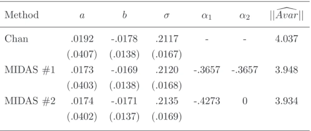
Table 2.1: Cox Ingersoll Ross Results
Method a b σ α1 α2 ||Avar[||
Chan .0192 -.0178 .2117 - - 4.037
(.0407) (.0138) (.0167)
MIDAS #1 .0173 -.0169 .2120 -.3657 -.3657 3.948 (.0403) (.0138) (.0168)
MIDAS #2 .0174 -.0171 .2135 -.4273 0 3.934 (.0402) (.0137) (.0169)
Figure 2.1: MIDAS 1 Weights
0 5 10 15 20
0 0.05 0.1 0.15 0.2 0.25 0.3 0.35
Lagged Yield
Weight
The improvement in the standard errors is minimal. In order to shrink the norm of the
Figure 2.2: MIDAS 2 Weights
0 5 10 15 20
0 0.05 0.1 0.15 0.2 0.25 0.3 0.35
Lagged Yield
Weight
ε1 weight ε2 weight
asymptotic variance, the standard errors in estimation ofσ increase in order to get a decrease
in standard errors for a. Whether or not this is an improvement is unclear.
As constructed, the following weighting scheme for the parameters αmean that in the case
of the first specification of MIDAS instruments, there is downward weighting as lag length
increases. The most recent yields are given more weight than the less recent ones. The
Cox-Ingersoll-Ross Model of the term structure is a Markov order one model, which means the
price of the asset at timetis sufficient information to describe the current state of the world.
The fact that some yields from the previous period are valuable as an instrument in terms of
minimizing the asymptotic variance is evidence that the model is misspecified. Given that the
model is a discrete time approximation of a continuous time process, this is not surprising.
Once different parameters are allowed for the error term and for the volatility, the optimal
MIDAS weighting parameter for the error remains a downward weighting scheme, but the
parameter for the volatility instead is essentially an even weight of each of the past 20 days’
monthly yields. This indicates that there is some persistence in the volatility, and perhaps a
more sophisticated stochastic volatility model would be preferable. Not only is there an issue
with the discretization, but perhaps the fundamental model is incorrect and the process is not
that this is the case.
2.3.2 Integrated Volatility
In Bollerslev and Zhou (2002) a stochastic volatility model is estimated by GMM. The log
price processpt is defined as follows:
dpt = µtdt+
p
VtdBt
dVt = κ(θ−Vt)dt+σ
p
VtdWt
whereVt is a scalar latent volatility process,µt is the mean and (dBt, dWt) are two brownian
motions. The parameter κ is considered to be the mean reversion parameter, θ the long run
mean of the volatility process, andσ the volatility of the volatility. In order for the process to
be well defined, it is required that κ >0,θ >0, andσ2 ≤2κθ.
The fundamental issue facing estimation of stochastic volatility models by GMM is that the
volatility processVt is unobservable. As a result, usually alternative estimation techniques are
utilized like Efficient Method of Moments (EMM) and Markov Chain Monte Carlo estimation
(MCMC). However, if there are several high frequency observations of the log price pt, then
one can find an estimate for the quadratic variation from timetto T, defined as follows:
[p, p]GT −[p, p]Gt ≡ lim ||G||→0
P
X
i=1 h
pt+i
P(T−t)−pt+ i−1
P (T−t)
i2
where G is the partition of the interval from t to T, ||G|| is the mesh of G (the size of the
longest subinterval), andP is the number of subintervals fromttoT. The theory of quadratic
variation says that :
lim
N→∞
2N
X
i=1 h
pt+ i
2N(T−t)−pt+ i−1 2N(T−t)
i2 →a.s.
Z T
t
v(ps, Vs, s;ξ)ds=Vt,T
. In other words, the quadratic variation for finer and finer frequency observations converges
in the limit to the integrated volatility from timet to T.
So if there is a high frequency data set with many intradaily observations for a particular
asset, an econometrician can find the integrated volatility Vt,T from day t to day t+ 1 (or
any future dayT) by taking the sum of the differences in log price squared. For example, the
Euro to U.S. Dollar (Euro/Dollar, price of Euros in Dollars) exchange rate observed every ten
minutes over a 24 hour period is used in this section to estimate the integrated volatility of the
log price process over the course of a day. If this data set is of a sufficiently high frequency, the
integrated volatility can effectively be treated as observable. Bollerslev and Zhou normalize
and consider (T −t) as one day, and define the integrated volatility over the course of a day
as Vt,t+1 = PPi=1 h
pt+i P −pt+
i−1 P
i2
where P is the number of intraperiod intervals observed.
With an observable integrated volatility process, a GMM estimator can be derived.
Bollerslev and Zhou define a vector of moments as follows:
ht(ξ) =
E[Vt+1,t+2|Gt]− Vt+1,t+2
E[V2
t+1,t+2|Gt]− Vt2+1,t+2
Where Gt is the sigma algebra generated by only being able to observe the log price process
pt (and thus the integrated volatility). The symbol ξ represents the vector of parameters.
Note that by construction the conditional expectation of ht(ξ) on Gt is zero. They derive
the following form for the conditional moments E[Vt+1,t+2|Gt] and E[Vt2+1,t+2|Gt]. For more
information on these derivations consult their appendix:
E[Vt+1,t+2|Gt] = αE[Vt,t+1|Gt] +β
where
α = e−κ
β = θ(1−e−κ)
H = e−2κ
I = 1
a[a
2(C+ 2αβ) + (α−α2)(2αβ+A)]
J = −b
a[a
2(C+ 2αβ) + (α−α2)(2ab+A)] + [a2(D+β2) +β(2ab+A) + (1−α2)(b2+B)]
and
a = 1
κ(1−e
−κ)
b = θ− θ κ(1−e
−κ)
A = σ
2
κ2[
1
κ −2e
−κ− 1 κe
−2κ]
B = σ
2
κ2[θ(1 + 2e
−κ) + θ
2κ(e
−κ+ 5)(e−κ−1)]
C = σ
2
κ (e
−κ−e−2κ)
D = σ
2θ
2κ (1−e
−κ)2
So it is possible to construct a two dimensional vector ht(ξ) defined as:
ht(ξ) =
αE[Vt,t+1|Gt] +β− Vt+1,t+2
HE[V2
t,t+1|Gt] +IE[Vt,t+1|Gt] +J− Vt2+1,t+2
with three parameters to estimate: κ, θ, and σ. Note thatht(ξ) is expected to be zero
condi-tionally on the observable information at timet(Gt). This lends itself to instrumental variables
estimation, where any variables known at tare applicable. Bollerslev and Zhou construct the
following moment conditions with the integrated volatility from time t−1 to time t:
gt(ξ) =
ht,1(ξ)
ht,2(ξ)
Vt−1,tht,1(ξ)
Vt−1,tht,2(ξ)
Vt2−1,tht,1(ξ)
Vt2−1,tht,2(ξ) = 0
which has 6 moment conditions for 3 parameters so the model can be estimated. This
disserta-tion improves this estimadisserta-tion by replacing the instruments with MIDAS instruments. Instead
of Vt−1,t consider the instrument with normalized Almon weights defined as follows:
zt(γ) =b(γ, L)(4pt)2 =
P
PP j=1eγj
∗ P
X
i=1 h
eγi(pt−1+i
P −pt−1+ i−1
P ) 2i = P X i=1 h
wi(pt−1+i
P −pt−1+ i−1
P )
2i
In other words, replace the integrated volatility over the last period as an instrument with
a weighted sum of the log price differences squared. The sum of the weights are normalized
to be equal to P, which is equivalent to the sum of the weights used to find the quadratic
variation, i.e. equal weighting. These weights are completely described by the parameter γ.
The parameterγ is found by the MIDAS instruments procedure outlined in this chapter. The
following are the moment conditions used in estimation:
gt(γ;ξ) =
ht,1(ξ)
ht,2(ξ)
zt(γ)ht,1(ξ)
zt(γ)ht,2(ξ)
zt(γ)2ht,1(ξ)
zt(γ)2ht,2(ξ)
Figure 2.3: Daily Integrated Volatility Euro
0 200 400 600 800 1000 1200 1400 1600 1800 0
1 2 3 4 5 6 7 8x 10
−4
time t Realized Volatility Euro
from August 3rd 2008 to September 2nd 2010 is collected from Forexrate.co.uk. After removing
poor data due to holidays, missing values etc, there are 1815 days worth of data, almost
always with 144 intradaily ten minute sampled observations for the 24 hour trading day. The
integrated volatility is graphed in Figures 2.3 and 2.4. This data is used to estimate the
parameters of the simple stochastic volatility model outlined earlier, first using the previous
day’s integrated volatility as an instrument, and then using the MIDAS instruments procedure.
Results are listed in Tables 2.2 and 2.3. Note that in both cases, the requirements thatκ >0,
θ >0, andσ2 ≤2κθ are satisfied.
Table 2.2: Integrated Volatility Results: Euro
Method κ θ σ γ ||Avar[||
B and Z .2526 2.778 ×10⁻⁵ -.0030 - .4293
(.0153) (3.573 ×10⁻⁶) (2.195 ×10⁻⁵)
MIDAS .2714 2.781 ×10⁻⁵ -.0031 .0090 .2731 (.0122) (3.589 ×10⁻⁶) (1.676 ×10⁻⁵)
Figure 2.4: Daily Integrated Volatility Yen
0 200 400 600 800 1000 1200 1400 1600 1800 0
0.1 0.2 0.3 0.4 0.5 0.6 0.7 0.8 0.9
1x 10
−3
time t Realized Volatility Yen
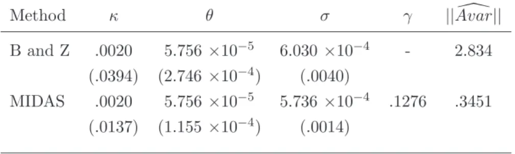
Table 2.3: Integrated Volatility Results: Yen
Method κ θ σ γ ||Avar[||
B and Z .0020 5.756×10⁻⁵ 6.030×10⁻⁴ - 2.834
(.0394) (2.746 ×10⁻⁴) (.0040)
MIDAS .0020 5.756×10⁻⁵ 5.736×10⁻⁴ .1276 .3451 (.0137) (1.155 ×10⁻⁴) (.0014)
The first conclusion from looking at the results is that the estimates are basically identical
for both procedures, which is to be expected since both procedures lead to consistent estimates.
In both cases there is a clear improvement in the size of the standard errors, in particular for
the case of the Yen/Dollar exchange rate. Since ifα was 0, the MIDAS specification would be
identical to Bollerslev and Zhou’s, it only makes sense that there would be improvements in
the asymptotic standard errors. Looking at the MIDAS weighting scheme, in both cases a lot
of weight is put on the trades made from midnight to 4:00 AM the previous trading day. Since
Figure 2.5: MIDAS Weights Euro
0 50 100 150
0.4 0.6 0.8 1 1.2 1.4 1.6 1.8 2
Value of i for Lagged Observation t − i/P (10 minutes)
Weights
MIDAS Weights over Log Price Difference Squared
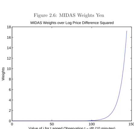
Figure 2.6: MIDAS Weights Yen
0 50 100 150
0 2 4 6 8 10 12 14 16 18
Value of i for Lagged Observation t − i/P (10 minutes)
Weights
MIDAS Weights over Log Price Difference Squared
Time in London, Midnight to 4 AM is equivalent to 9 AM to 1 PM in Japan, and roughly
5PM to 9PM in America. Thus the weighting for the Yen makes sense, but the weighting for
Euro is counter intuitive.
2.4 Conclusion
The MIDAS Instruments methodology for more than one parameter gives improved asymptotic
standard errors by construction. It chooses instruments for the explicit purpose of minimizing
those standard errors, or rather, the estimate of those standard errors from a given sample.
Since in both empirical examples, the MIDAS Instruments methodology nests the initial
in-strumental variables estimation procedure (choose αnegative and very large in absolute value
for Term Structure example, choose γ = 0 for integrated volatility example) this procedure
chooses better instruments for estimation. An econometrician cannot do worse by applying
this methodology, given the model is correctly specified. Since almost any weighting scheme
can be considered, this gives a very large framework for improved estimation.
Martingale difference sequence errors are quite common in many time series models, and
even if mixed frequency data is not admissible, the methodology can be applied to a weighted
sum or average of lagged instruments with identical sampling frequency as the initial time
series. In fact, the basic idea could even be applied in a non time series context. As long as
the expectation of a function is zero given more than one instrument, there is a parameterized
Chapter 3
Optimal MIDAS Instruments for MDS Errors
3.1 Motivation
The large majority of discrete time asset pricing models are only concerned with time series of
a fixed sampling frequency. By only considering data occurring at a single time frequency, a lot
of information available to agents in the economy is ignored by the models. This information
is potentially very useful in properly pricing assets. This chapter combines time series of
different fixed frequencies in order to improve parameter estimation and testing of discrete
time asset pricing models with martingale difference sequence errors. The goal is accomplished
by considering the optimal instruments, in other words the instruments which are theoretically
efficient given the assumptions.
Hansen and Richard (1987) showed that under suitable regularity conditions there is a
unique stochastic discount factor (SDF) mt+1(θ0) that prices all payoffs (in a given payoff
space) according to:
E[mt+1(θ0)Rt+1|Jt] = ι
where Jt is the information set of agents in the economy and Rt is an N-vector (with ι a
unit vector of the same dimension) of so called test assets used to estimate, test or appraise
the empirical specification. The econometric implementation of the above model uses a GMM
estimation procedure involving instrumental variables and amounts to conditioning down the
above fundamental pricing equation to an information set that typically consists of lagged
This means that a model estimated with quarterly data usually involves lagged quarterly
re-turns and consumption as instruments. The assumption of quarterly pricing kernal estimation
does not imply that instruments should involve data sampled at the same frequency. Agents
know much more than past quarterly consumption.
To illustrate this further, consider the pricing of a single asset (i.e.N = 1) and let quarterly
log per capita consumption growth be the sum of three monthly log per capita consumption
growths in quarterly ∆t: ∆ct≡∆c(1)t + ∆c (2) t + ∆c
(3)
t ,where ∆c (i)
t refers to the change in log
consumption in month iof quarter t. Typically the econometrician will consider the moment
conditions:
E[(mt+1(θ0)Rt+1−1)×
1
∆c(1)t + ∆c(2)t + ∆c(3)t
Rt
] = 0
where Rt is the previous quarter’s return. Denote the information set by JtLF when it only
consists of same/low frequency data, or formally:
JtLF =σ({Rt−i}i=0,1,..,{∆ct−i}i=0,1,..,{xt−i}i=0,1,..)
where {xt} is a time series vector of data assumed to be known and of interest to the
repre-sentative agent.
Break down variable ∆ctinto its individual terms, and construct new instruments and new
moment conditions:
E[(mt+1(θ0)Rt+1−1)×
∆c(1)t
∆c(2)t
∆c(3)t
] = 0
As such consider a mixed frequencyJM F
t information setting, defined as:
JtM F =σ({R(t−j)i}{i=0,1,..,j=1,2,...,NR},{∆c
(j)
where the letter iindicates the quarter, andj represents a higher frequency past observation
within that quarter. The highest frequency consumption reported is monthly thus j can only
equal 3 at most for consumption observations, but returns and{x(tj−)i}may be recorded at much
higher frequencies within a given quarter. Is this instrument choice necessarily inadmissible
just because ∆c(tj) is a monthly time series instead of quarterly?
The notion that higher frequency data being utilized generates a host of interesting
is-sues. It is desirable to avoid large dimensional estimation problems, where a multitude
of moments are constructed, using many potentially redundant or weak instruments (see
e.g. Koenker and Machado (1999), Han and Phillips (2006), Newey and Windmeijer (2009),
among others). Therefore one may wonder how to use high frequency data without a
pro-liferation of moment conditions. What about optimal GMM instruments? It turns out that
the very notion of optimal GMM instruments (see e.g. Chamberlain (1987), Hansen (1985),
Hansen, Heaton, and Ogaki(1988),Hansen and Singelton(1996), among others) is for a given
data filtration. If the filtration changes, the design of optimal instruments potentially change
as well. This chapter will show how to address this - namely how to take advantage of mixed
frequency data to construct more efficient optimal instruments. In fact, this chapter will show
that under suitable regularity conditions, there will always be improvements in terms of
effi-ciency and therefore specification tests with better (local asymptotic) power can be designed.
While the idea of using mixed frequency data is generic, this chapter will primarily focus on
situations where one also knows how to construct optimal instruments. In particular, the case
of affine SDFs as inNagel and Singleton(2011) is considered, i.e.mt+1(θ0) =θ0ft+1whereft+1
are stochastic risk factors (components within{xt−i}). The parameters are estimated using the
optimal choice of instruments in IV estimation, i.e. the instruments such that the asymptotic
covariance matrix is smallest among all GMM estimators. In the case of an affine SDF, the
form of the optimal instrument,A∗t =Eh∂ht+1(θ0)
∂θ |Jt
i
(V art[ht+1(θ0)])−1 is known. Note that
this instrument is the product of two conditional moments. As such the optimal instrument is
fundamentally determined by the corresponding conditional information set or filtration. An
econometrician who uses Jt=JtLF in estimation has a different optimal instrument than one
usingJt=JtM F or any other feasible filtration defined by the model, since A∗t will clearly be
different depending on the choice of Jt. Thus using the optimal instruments for estimation
requires choosing a filtration. In other words, efficiency is not just a matter of
implement-ing optimal instruments, but also decidimplement-ing what exactly is the conditionimplement-ing information and
considering the corresponding optimal instruments for that information.
In particular, this chapter considers the optimal instruments for a given filtration and the
corresponding conditional moments that go into its construction. In addition, it considers
the corresponding optimal Wald and Lagrange Multiplier hypothesis tests as described in
Nagel and Singleton (2011) and proves under suitable regularity conditions that considering
optimal instruments using a mixed frequency filtration as opposed to a low frequency one
leads to a more powerful test under local alternatives. The notion of psuedo-higher frequency
horizon test assets are also introduced in order to potentially improve estimation. These test
assets of a pseudo-higher frequency horizon are low frequency horizon test assets, but are
constructed in such a way that the traditional low frequency portfolio assets can be considered
as buying and selling these higher frequency assets at different points throughout the model’s
horizon.
Finally, the methodology is applied to the empirical application of Nagel and Singleton
(2011) to find smaller asymptotic standard errors for parameter estimates and a more powerful
Wald and Lagrange Multiplier test.
3.2 Affine SDFs and Optimal Instruments
Under fairly mild conditions pertaining to the absence of arbitrage and the law of one price,
Hansen and Richard (1987) show that there is a unique stochastic discount factor (SDF)
mt+1(θ0) that prices all payoffs (in a given payoff space) according to:
E[mt+1(θ0)Rt+1|Jt] = ι
where Rt+1 is an N sized vector of gross asset returns,ι is an N sized unit vector, and Jt is
the information set of the representative agent. The particular class of mt+1(θ0) of interest
assuming a mixed frequency Jtand its implications on hypothesis testing follows.
3.2.1 Model and GMM Estimation
Various models define mt+1 differently, but recently, Nagel and Singleton (2011) focused on
SDFs that are affine in ft,a set of observed priced factors, in particular:
mt+1(θ0) = θ00ft+1 (3.1)
where ft+1 is aM ×1 vector of conditional risk factors. The parameters of interest θ can be
written using two subvectors β and γ such that:
mt+1(θ0) = mt+1(β0, γ0) (3.2)
mt+1(θ0) = β00fβ,t+1+γ00fγ,t+1 (3.3)
The parameter vector θ0 is broken into two separate subvectors for the purpose of hypothesis
testing later, namely to test the null hypothesis that γ0 = 0. An example of an affine SDF
would be:
mt+1(θ0) = (θ10+θ02at) + (θ03+θ04at)∆ct+1 (3.4)
where ∆ct is quarterly consumption growth, whereas various choices for at include but are
not limited to the consumption-wealth ratio of Lettau and Ludvigson (2001), the corporate
bond spread of Jagannathan and Wang (1996), or the labor income-consumption ratio of
Santos and Veronesi (2006). With this definition of the stochastic discount factor, define a
pricing error vector as:
ht+1(θ0) = mt+1(θ0)Rt+1−ι (3.5)
It is clear that the following holds:
E[ht+1(θ0)|Jt] = 0N (3.6)
where 0N is aN×1 vector of zeros. This states that the pricing error is a martingale difference
sequence with respect to the information setJt. If any matrixAt ∈Jtsuch that At isK2 ×N
(K2 ≥ K where K is the dimension of θ), and E[At(∂ht+1(θ0)/∂θ)] has full rank then At is
an admissible instrument for GMM estimation according to the moment condition:
E[Atht+1(θ0)] = 0 (3.7)
For any admissible instrument At, the GMM estimate (with optimal weighting matrix) forθ0
is defined as:
ˆ
θA = argmin
θ
1
T T
X
t=1
Atht+1(θ) !0
(ΣbA0)−1 1
T T
X
t=1
Atht+1(θ) !
(3.8)
whereT is the number of observations, andΣbA
0 is a consistent estimate of the matrix
ΣA
0 = E
Atht+1(θ0)ht+1(θ)0A0t
(3.9)
and the asymptotic covariance matrix for the estimator is
ΩA
0 = E
At
∂ht+1(θ0) ∂θ
−1
ΣA 0E
∂h
t+1(θ0)0 ∂θ A
0
t
−1
(3.10)
No matter what admissible instrument is chosen, under regularity conditions, ˆθA will be a
consistent estimate of θ0. Nagel and Singleton (2011) advocate the use of optimal GMM
instruments to exploit the pricing equation more efficiently. As shown inChamberlain(1987),
Hansen (1985), and Hansen, Heaton, and Ogaki (1988), the optimal instrument which leads
to the asymptotically efficient estimator for a martingale difference sequence is as follows.
where
Ψθt0 ≡ E
∂ht+1(θ0) ∂θ
Jt
0
(3.12)
Σt ≡ Eht+1(θ0)ht+1(θ0)0|Jt (3.13)
≡ V ar[ht+1(θ0)|Jt] (3.14)
This instrument is the conditional score multiplied by the inverse of the conditional variance
of the error term. The first term in the instrument captures the sensitivity of the error to
changes in parameters whereas the second normalizes the error’s conditional variance to a unit
vector. This instrument is not traditionally found in Jt, as a result, feasible estimates must
be used instead in application. This chapter aims to construct better, more feasible estimates
for the optimal instrument by reconsidering the form of Jt and allowing for mixed frequency
observations to be in the information set. The methodology section outlines the procedure
used for estimation.
With these instruments the asymptotic covariance matrix for the estimator simplifies to
ΩA0∗ = E[Ψθt0Σ−t1Ψθt]−1 (3.15)
Nagel and Singleton (2011) estimate the conditional moments using local polynomial
regres-sion and a global polynomial approximation.
As noted before, the approach of Nagel and Singleton (2011) can be characterized as
using the information set JLF
t with same/low frequency data. The instruments are
con-structed from data of the same frequency as the error term. How can one formulate
in-struments with the mixed frequency filtration JM F
t and take advantage of all the
informa-tion known to the representative investor? This chapter uses an extension of the MIDAS
framework introduced in Ghysels, Santa-Clara, and Valkanov(2005) and further developed in
Andreou, Ghysels, and Kourtellos (2010) to accomplish this. For introductory purposes, first
consider the circumstances when Rt+1 is a scalar. In this case the first part of the optimal
instrument becomes:
E
∂ht+1(θ0) ∂θ |J
M F t
0
= E
∂(θ00ft+1)Rt+1−1
∂θ |J
M F t
0
= Eft+1Rt+1|JtM F
0
which is aK×1 vector of conditional moments:
E
f1,t+1Rt+1
.
fK,t+1Rt+1 |
JtM F
Similarly the second part of the optimal instrument becomes (if not considering the inverse
just yet):
V arht+1(θ0)|JtM F
= V ar(θ00ft+1)Rt+1−1|JtM F
= V ar(θ00ft+1)Rt+1|JtM F
=
K
X
i=1
θ20,iV arfi,t+1Rt+1|JtM F
+2X
i6=j
θ0,iθ0,jCov[fj,t+1Rt+1, fi,t+1Rt+1|JtM F]
Which requires the estimation of the following K×K covariance matrix:
V ar
f1,t+1Rt+1
.
fK,t+1Rt+1 |J
M F t
To deal with the potential large cross-section of daily series contained withinJtM F,Andreou, Ghysels, and Kourtellos
(2010) proposes to run ADL-MIDAS regressions, selecting one series from five main classes of
assets - equities, foreign exchange, corporate risk, commodities prices and fixed income - and
then combine the regression predictions via model averaging. The assets used in the
limited to two sets of data: a set of time series beginning in 1986, and another set beginning
in 1999. The reason for the two separate sets is that paper only considers model averaging
for forecasts involving data sets of the exact same length even though more and more daily
data becomes available at different times throughout the time frame of interest. Instead here
this procedure is augmented by constantly incorporating the newer model predictions as they
become available, such that more models are averaged as the prediction comes closer to the
present day, and data is not separated depending on availability. More detail on this procedure
is given in the methodology section.
In the case where the pricing error is not a scalar, ADL-MIDAS regressions are used in
order to estimate the new expected partial derivatives and all the covariance (off diagonal)
terms in the pricing error’s conditional covariance matrix. Namely the following conditional
moments need to be found:
E
ft+1Ri,t+1
|JtM F
for all asset returns indexed by iand
Cov(fm,t+1Ri,t+1, fn,t+1Rj,t+1|JtM F)
for all asset returns indexed byi, j, and risk factors indexed bym, n. This information can
be thought of as residing in a 4 dimensional array, which is less convenient than simply being
a matrix as in the case whereN = 1. Notice that if N = 1 then this simplifies to determining
the conditional moments and covariance matrix outlined earlier. Although conceiving of a 4
dimensional array is less convenient, the principle remains the same. The optimal instrument
simply consists of a number of conditional moments which have to be properly constructed
and ordered. Creating the optimal instrument entails estimating the conditional moments and
organizing them as the product of K ×N matrix Ψt and the N ×N matrix Σt. Thus as
before, ADL-MIDAS regressions are used for the new conditional moments of interest and to
construct these matrices. Using these MIDAS estimates for the conditional forecasts one can
construct the two matrices that composeA∗
t and estimate the parameters of interest using the
instrument known to be optimal.
Now consider the situation whenN >1 and the test assets are expressed in a vector. The
first part of the optimal instrument becomes:
E
∂ht+1(θ0) ∂θ |J
M F t
0
= E
∂(θ00ft+1)Rt+1−1
∂θ |J
M F t 0 = E
f1,t+1R1,t+1 ... f1,t+1RN,t+1
f2,t+1R1,t+1 ... f2,t+1RN,t+1
. ... .
fK,t+1R1,t+1 ... fK,t+1RN,t+1 |JtM F
0
which is aK×N vector of conditional moments.
The second part of the optimal instrument becomes (before taking the inverse):
V arht+1(θ0)|JtM F
= V ar(θ00ft+1)Rt+1−ι|JtM F
This is a N×N conditional covariance matrix. The diagonal element (m, m) is:
Σt,(m,m) = V ar(θ00ft+1)Rm,t+1−1|JtM F
=
K
X
i=1
θ02,iV arfi,t+1Rm,t+1|JtM F
+2X
i6=j
θ0,iθ0,jCov[fj,t+1Rm,t+1, fi,t+1Rm,t+1|JtM F]
and the off diagonal element (m, n), m6=nis:
Σt,(m,n) = Cov
(θ00ft+1)Rm,t+1−1,(θ00ft+1)Rn,t+1−1|JtM F
= K X i=1 K X j=1
θ0,iθ0,jCovfi,t+1Rm,t+1, fj,t+1Rn,t+1|JtM F
Thus to assemble all the moments that are contained in Σtfor all factorsi, jand test assets
Cov(fm,t+1Ri,t+1, fm,t+1Rj,t+1|JtM F)
3.2.2 Hypothesis Testing
After the estimates for the optimal instruments and the resulting GMM estimator are
assem-bled, consider the relevant hypothesis tests for the estimator. Consider the parameters θ0,
which can be broken into two subvectors β0 andγ0. The hypothesis test is whether or not γ0
is composed of zeros. DefineGto be the dimension ofγ0and ΩAγγ to be theG×Gsubmatrix of
the asymptotic covariance matrix, i.e. ΩAγγ =RWΩAR0W whereRW is aK dimensional vector
of ones (if θi is part ofγ) and zeros (otherwise). If the corresponding Wald statistic is defined
asWT(A∗), then under the null hypothesisH0 :γ0 = 0 the following holds:
WT(A)≡ T γT0 ΩAγγ
−1 γT
D
→χ2(G) (3.16)
As inNagel and Singleton (2011) the local power of this test is under consideration. Consider
a local alternative H1T : γ0 = δ/ √
T where δ is some nonzero G×1 vector. Under the
local alternative, since √T(γA
T −γ0)→ N(δ,ΩAγγ), the asymptotic distribution of ςTW(A) is a
noncentral chi-square distribution with non-centrality parameter as follows:
N C(A) = δ0(ΩAγγ)−1δ (3.17)
N C(A) = δ0(RWΩAR0W)−1δ (3.18)
This holds for any instrumentAthus it also holds for the optimal instrumentA∗and any
stand-in optimal stand-instrument estimate constructed from the stand-information set JM F
t . The question is
whether or not certain constructed optimal instruments result in more powerful Wald tests
than others. If a decomposition is employed as in Engle(2002) andHalbleib and Voev (2011)
of the conditional covariance matrix Σt to DtRtDt where Dt is a diagonal matrix of positive
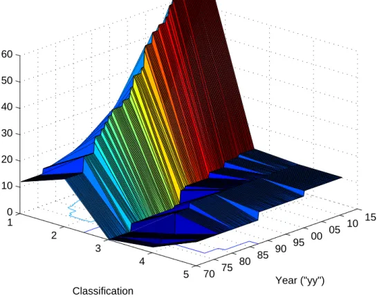
![Figure 3.4: Average weight within each Time Series classification in forecast of E t [R t+1 ] 1 2 3 4 5 70 75 80 85 90 95 00 05 10 1500.010.020.030.040.05 Year ("yy") Classification](https://thumb-us.123doks.com/thumbv2/123dok_us/8269783.2190472/59.918.192.752.168.600/figure-average-weight-time-series-classification-forecast-classification.webp)
![Table 3.3: Optimal for Market, Augmented by Risk Free Moment Affine SDF J Stat θ 1 θ 2 θ 3 θ 4 Wald LM Almon Σ t cay 0.17 1.16 2.29 -40.95 713.22 414.05 2.99 (0.035) (4.78) (1.62) (213.27) [1.00] [0.78] def 0.0036 2.51 -82.06 -219.53 8158.45 187.22 35.07 (](https://thumb-us.123doks.com/thumbv2/123dok_us/8269783.2190472/65.918.147.778.185.643/table-optimal-market-augmented-risk-moment-affine-almon.webp)

