Audio-Visual Particle Flow SMC-PHD Filtering for
Multi-Speaker Tracking
Yang Liu,
Student Member, IEEE,
Volkan Kılıc¸, Jian Guan, Wenwu Wang,
Senior Member, IEEE,
Abstract—Sequential Monte Carlo probability hypothesis den-sity (SMC-PHD) filtering is a popular method used recently for audio-visual (AV) multi-speaker tracking. However, due to the weight degeneracy problem, the posterior distribution can be represented poorly by the estimated probability, when only a few particles are present around the peak of the likelihood density function. To address this issue, we propose a new framework where particle flow (PF) is used to migrate particles smoothly from the prior to the posterior probability density. We consider both zero and non-zero diffusion particle flows (ZPF/NPF), and developed two new algorithms, AV-ZPF-SMC-PHD and AV-NPF-SMC-PHD, where the speaker states from the previous frames are also considered for particle relocation. The proposed algorithms are compared systematically with several baseline tracking meth-ods using the AV16.3, AVDIAR and CLEAR datasets, and are shown to offer improved tracking accuracy and average effective sample size (ESS).
Index Terms—Audio-Visual Tracking, Sequential Monte Carlo, PHD filter, Particle Flow, Optimal Proposal Distribution.
I. INTRODUCTION
M
ULTI-SPEAKER tracking has drawn increasing atten-tion in applicaatten-tions, such as security surveillance [1], and human-computer interaction [2]. However, the measure-ments used in multi-speaker tracking, either audio [3] or visual [4], often contain noise, clutter, and missing data [5], [6]. For example, in visual tracking, the tracking result is often affected by occlusions and the limited field of view of cameras [4], while in audio tracking, speakers are not always detectable when strong background noise and room reverberations are present in the measurements or when the speakers are silent.To address this problem, different modalities can be ex-ploited jointly for their complementarity. For example, speak-ers can be tracked using audio information, if they are vi-sually occluded, likewise, they can be tracked with visual information, when the audio information becomes unreliable, e.g. due to the presence of acoustic noise. Other modalities, such as thermal vision and laser rangefinders, could also be considered, however, we will focus on audio-visual sensors, as in [7], due to their widespread use, low cost, and easy installation [8]. More specifically, in our work, we consider the visual measurements obtained by the CAMShift [9] or a Y. Liu and W. Wang are with the Centre for Vision, Speech and Signal Pro-cessing, University of Surrey, Guildford, GU2 7XH, U.K. E-mails:{yangliu, w.wang}@surrey.ac.uk.
V. Kılıc¸ is with Department of Electrical and Electronics Engineer-ing, Izmir Katip Celebi University, 35620 Cigli-Izmir, Turkey. E-mail: [email protected].
J. Guan is with College of Computer Science and Technology, Harbin Engineering University, Harbin, 150001, China. E-mail: [email protected].
face detector [10], and the audio measurements, such as the direction of arrival (DOA) of the sources [11].
To fuse the audio-visual data, the Bayesian inference frame-work is a popular choice, which provides an intuitive way for the estimation of speaker states [12] from the measurements. Early methods include the Kalman filter (KF) [13], extended Kalman filter (EKF) [14] and particle filter [15], which can be used for a fixed and known number of speakers, while more recent methods include random finite sets (RFS) [16], Gaussian mixture (GM) PHD filter [6], sequential Monte Carlo (SMC) PHD filter [17], cardinalized PHD filter [18], and generalized labeled multi-Bernoulli (GLMB) RFS [19], which can be employed to track an unknown and time-variant number of speakers. The SMC-PHD filter uses a set of random particles to estimate the posterior density, as a result, it often suffers from the weight degeneracy problem [20], i.e. the weights of most particles will become negligible, while only a few remain significant, during the iterations in the particle propagation process.
To address the issue, several ideas have been developed. The SMC methods exploit the most recent measurements or the unscented transformation to approximate the optimal proposal distribution and to minimize the variance of the importance weights, as in e.g. the auxiliary particle filter [21], unscented particle filter [22], auxiliary SMC-PHD filter [23] and unscented auxiliary cardinalized PHD filter [24]. Another idea is based on the Markov Chain Monte Carlo method [25], as performed in the well-known resample-move algorithm [26], where the particles are drawn to represent independent samples from the target posterior. Finally, an idea based on bridging densities [27], [28], [29] has also been developed for approaching the true posterior density from the tractable prior density. This method offers theoretical elegance and promising performance, but involves complicated approximation of the optimal bridging densities.
In this paper, we propose a new method to address the weight degeneracy issue, based on particle flow [30], [31], [32]. Different from the above-mentioned techniques, such as the popular particle re-sampling technique, our method aims to improve the effective sample size with a particle relocation strategy designed using particle flow. More specifically, the particles are migrated from the prior to the posterior distri-bution, using a homotopy function which defines the flow in synthetic time and incorporated for particle update at each time frame [33].
According to the different assumptions employed for solv-ing the homotopy function, particle flow can be divided into five classes: incompressible particle flow [34], zero diffusion
particle flow (ZPF) [32], Coulomb's law particle flow [35], zero-curvature particle flow [36] and non-zero diffusion par-ticle flow (NPF) [37]. In this work, we consider ZPF and NPF. The ZPF is easy to implement [38] and widely used [39], [40], [41]. NPF does not assume any particular form of the prior density and likelihood function [37]. NPF offers slightly better performance than ZPF. Note that, we do not consider the other types of particle flows for the following reasons. Incompressible particle flow equation only works on some special prior densities, such as Gaussian density [42]. Coulomb's law and zero-curvature particle flows are sensitive to initialization of the state vector [36].
Zero particle flow has been used previously to improve the particle filter by reducing the number of particles in the particle flow particle filter (PFPF) [43] and theδ-GLMB particle filter [44], and to improve the Gaussian mixture PHD filter in [29] for an unknown number of targets. However, there are several main differences between our proposed methods and these methods. First, particle flow is used to improve the SMC-PHD filter in our method, mainly for particle relocation and weight update in order to mitigate the weight degeneracy issue. Second, only ZPF has been considered in the previous methods, while we have also developed a new method using NPF. Third, the mean and covariance of the particles are es-timated by a clustering technique, while in previous methods, these are estimated using EKF [43], Gaussian mixture model [29], or label information [44]. Fourth, our proposed methods offer significant performance improvements and computational advantages compared with these previous methods.
To demonstrate the advantages of the proposed method, we consider a recent baseline i.e. audio-visual SMC-PHD (AV-SMC-PHD) filter introduced in [5], and developed two new algorithms, namely, AV-ZPF-SMC-PHD and AV-NPF-SMC-PHD. We compare systematically the proposed algorithms with several other state-of-the-art methods, such as the sparse-AVMS-SMC-PHD filter in [5], where mean-shift (MS) was used for particle relocation.
Preliminary results of this work were presented in confer-ence papers [20] [7] [45]. This paper provides a comprehensive treatment of the proposed methods together with new improve-ments and experimental results. First, the direction of arrival (DOA) and color histograms are both used for deriving the particle flow. When speakers are not detected with the DOA information or the color histograms, particle states can still be updated with particle flow. Second, the speaker states and weights in the previous frames are used for relocating particles in terms of DOA, in order to reduce the adverse impact of acoustic noise on particle relocation. Third, we perform extensive experiments on the AV16.3 [46], AVDIAR [47] and CLEAR [48] datasets, and compare the proposed method with several baseline methods including the PF-PF [41], ZPF-GPF-PHD [29], sparse-AVMS-SMC-PHD [5] filters, auxiliary SMC-PHD filter [23], and a deep learning based face detector [10].
This paper is organized as follows. The next section dis-cusses the problems and background. Section III presents the details of the proposed methods. In Section IV, the proposed algorithms are compared with several baseline algorithms
based on comprehensive experiments. Finally, Section V con-cludes the paper.
II. PROBLEMSTATEMENTANDBACKGROUND This section describes the problem formulation, the SMC-PHD filter, the particle flow filter, and a baseline AV-SMC-PHD algorithm. We assume that the speaker dynamics and measurements are described as a Markov state-space signal model: {m˜jk}N˜k j=1=Fm˜ {m˜jk−1}N˜k−1 j=1 ,τk (1) Zk =Fz {m˜jk}N˜k j=1,ςk +k (2)
wherem˜jk ∈RM represents the state vector for thejth speaker at timek, and ˜ is used to distinguish the speaker state from the particle state used later. The statem˜jk = [xjk, yjk,x˙jk,y˙jk]T consists of positions (xjk, yjk) and velocities ( ˙xjk,y˙kj), while the observation is a noisy version of the position. Hence M = 4. For 3D calculations, the speaker state is set as
˜ mjk = [xjk, yjk, wkj,x˙kj,y˙kj,w˙jk]T, where(xj k, y j k, w j k)is the 3D
position of the jth speaker and ( ˙xjk,y˙kj,w˙jk) is the speaker velocity. At time k, m˜jk is approximated by Nk particles
{mik}Nk
i=1 with weights {ω
i k}
Nk
i=1. Let Zk denote the set of
measurements at timek, defined as[{m˚ok}Ok
o=1,{m˘
u k}
Uk
u=1]for
audio-visual measurements, whereOk andUk are the number
of audio ˚ and visual ˘ measurements, respectively. τk
and ςk are system excitation and measurement noise terms,
respectively. k is the clutter term. Fm˜ is the transition
model and Fz is the nonlinear measurement model. A list
of important notations is given in Table I, whereo anduare the indices of audio and visual measurements.
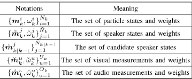
TABLE I: List of important Notations
Notations Meaning
{mik, ωik}Nk
i=1 The set of particle states and weights
{m˜jk,ω˜kj}N˜k
j=1 The set of speaker states and weights
{m˜jk|k−1}jN˜=1k|k−1 The set of candidate speaker states
{m˘u k,ω˘ku}
Uk
u=1 The set of visual measurements and weights
{m˚o k,˚ωok}
Ok
o=1 The set of audio measurements and weights
A. SMC-PHD filter
In the prediction step [49], the particles are obtained by the proposal distribution qk(mik|k−1|mik−1,Zk), with weights
ωki|k−1= φk|k−1(mik|k−1|m i k−1)ω i k−1 qk(mik|k−1|mik−1,Zk) , i= 1, ..., Nk−1 (3)
whereφk|k−1is the analogue of the state transition probability.
NB particles are sampled from the new born importance
functionpk with weights
ωki|k−1= γk(m i k|k−1) NBpk(mik|k−1|Zk) , i=Nk−1+ 1, . . . , Nk−1+NB (4)
where γk is the probability of the new born speaker, whose
integral approximates the average number of speakers in the state space. In the update step, the weights are calculated as
ωik= 1−piD,k+ X zr k∈Zk piD,khi,rk κk+P Nk i=1piD,kh i,r k ωki|k−1 ωki|k−1 (5) in which κk denotes the clutter intensity of the rth
measure-ment zr
k at time k. piD,k is the detection probability of the
ith particle at time k. κk and piD,k can be assumed known
a priori and constant as in [50]. Alternatively, a model of Beta-Gaussian mixtures can be used to estimate unknown κk
and pi
D,k as in [51]. h i,r
k is the likelihood of the ith particle
for the rth measurement, which can be estimated in terms of their Bhattacharyya distance [52] or Euclidean distance [53] with a Gaussian distribution. The number of speakers N˜k is
estimated as the sum of the weights. The states and weights of the speakers {m˜jk,ω˜kj}N˜k
j=1 can be calculated using e.g.
k-means clustering method [54] or multi-expected a posterior (MEAP) [55]. Finally, resampling is performed when the ESS is smaller than half of the number of particles. Resampling was proposed originally in [56] and popularised in [57]. According to the different strategies taken for selecting the particles, the resampling methods mainly fall into three cate-gories: multinomial resampling [58], residual resampling [58] and systematic resampling [59]. In multinomial resampling, the particles are independently selected and resampled. In residual resampling, the particles to be resampled are selected based on the values of their weights. In systematic resampling, the particles are clustered and the resampled particles are taken from each cluster. This can help reduce the discrepancy among the particles. The systematic resampling method has been used in the baseline SMC-PHD filter and will also be used in our proposed filter, due to its high resampling quality and low computational complexity.
B. Particle flow
In particle flow, a homotopy function is used to estimate the posterior density, as follows [33],
log(ψik) = log(g i k) +λlog(h i k)−logK i k (6) where Ki
k is the normalization constant independent of mik,
and λ, called pseudo time, is a step size parameter taking values from set [0,4λ,24λ,· · ·, Nλ4λ] and Nλ4λ = 1,
withNλbeing the number of pseudo time steps. In fact,λcan
also be variable step sizes as in [41], [32], which is further discussed in Section IV. Eq. (6) represents the evolution of the particles from the prior densitygik to the posterior density. When λ = 0, ψki represents the prior density gki at time k. When λ is varied to 1, ψik is translated into the normalized posterior density [30]. In ZPF, the posterior and likelihood function are assumed to be Gaussian and linear, and the flow
fi k,λ is derived as, fk,λi = dm i k|k−1 dλ =A i km i k|k−1+b i k (7) where Aik=− 1 2C i k λHkiP i k|k−1(H i k) T +R −1 Hki, (8) bik = I+ 2λAik h I+λAik CkiR−1zkr+Aikm¯ik|k−1 i (9) Cki =Pki|k−1(Hki)T (10) wherePi
k|k−1 is the covariance matrix of the prediction error
for the particle state mi
k|k−1, m¯
i
k|k−1 is the mean of the
states over the particle set, R is the covariance matrix of the measurement noise,I is the identity matrix, andHi
k is a
Jacobian matrix [60]. The details about ZPF are given in [33]. ZPF has been widely used for its simplicity. For nonlinear problems, this flow can be used to linearize the measurement equation for each particle with an extended Kalman filter. The main critical parameters in ZPF are the number of particles and the tolerance for the step-size selection. As a result, only little effort is required for parameter tuning.
Different from ZPF, the particle flow equation used in NPF is derived by retaining the diffusion term, as detailed in [37], given as follows, fk,λi =−[∇2logψi k] −1(∇loghi k) (11) where ∇2logψik≈ −(Pki|k−1)−1+λ∇2loghik (12) where ∇ is the spatial vector differential operator ∂mi∂
k|k−1
. hi
kis the likelihood of theith particle at timek. As compared
to ZPF, the prior density and likelihood function in NPF need to be sufficiently smooth [61], and the performance NPF tends to be more sensitive to the choice of parameters e.g. the pseudo-time step size. However, once properly tuned, NPF offers a lower computational cost and slightly better performance than ZPF. Therefore, NPF is also implemented in this work. It is worth noting that, other ideas are emerging to address the issues in NPF. For example, stochastic particle flow based on Langevin diffusion, has been proposed in [62], and the Gromovs method has been used to reduce sensitivity to parameter choice of NPF in [63]. These new developments make NPF an increasingly attractive choice.
C. AV-SMC-PHD filter
The SMC-PHD filter was recently used in [5] for multi-speaker tracking, based on the fusion of audio-visual in-formation. The audio information used is the DOA, e.g. the approximate direction of the speakers with respect to a microphone array, which can be detected by e.g. the sam-spare-mean (SSM) method [64], which is a joint detection and localization method, where the space is divided into sectors, with each sector corresponding to a certain direction, and the active sources are searched over these sectors in terms of the sound energy presented. Color histogram has been used as the visual information [5].
To fuse the audio-visual information, the surviving particles are relocated around the DOA lines which are drawn from the centre of the microphone array to points in the image frame
estimated by the projection of DOAs to a 2D image plane [65]. The visual information is used to estimate the likelihood function and to update the particle weights by Eq. (5).
More specifically, the distance for particle movement di k is calculated as: dik= ´ di k PNk−1 i=i d´ik ´ dik (13)
where d´ik is the perpendicular Euclidean distance from the particles to the DOA line [5], assuming the DOA line is avail-able at time k. Then, the surviving particles {mik|k−1}Nk−1
i=1
are relocated to near the DOA line [5] in terms of dik as:
mik|k−1⇐mik|k−1+okdik (14)
whereok= [cos(θko),sin(θko),0,0]T andθkois the
correspond-ing oth DOA angle. The visual information is used to derive the likelihood which is then used to update the weights ωi
k.
The pseudo code of baseline AV-SMC-PHD filter [5] is given in Algorithm 1, where T is the length of a frame.
Algorithm 1 AV-SMC-PHD Filter
Input:{mi
k−1, ωik−1}
Nk−1
i=1 ,NB,Zk,kand DOA lines.
Output: {m˜jk,ω˜kj}N˜k
j=1, and{mik, ωik} Nk
i=1.
Initialize: τk, qk, φk|k−1, pk, γk, κk, PD,k, Fm˜, Fz, T
and speaker histograms.
Run:
Step 1: Propagation step
Propagate surviving particles{mik|k−1}Nk−1
i=1 . Step 2: Particle birth and relocation step if DOA lines existthenCalculate dk by Eq. (13).
Concentrate particles around the DOA line by Eq. (14).
if new speakerthen SampleNB born particles
{mi k|k−1, ω
i k|k−1}
Nk−1+NB
i=Nk−1+1 uniformly around the
DOA line Eq. (4). Calculate {ωi
k|k−1}
Nk−1
i=1 by Eq. (3). Step 3: Prediction step
{mi k|k−1, ω i k|k−1} Nk i=1 = {mik|k−1, ω i k|k−1} Nk−1 i=1 ∪ {mik|k−1, ωki|k−1}Nk−1+NB i=Nk−1+1.
Step 4: Update step
Estimate colour likelihood.
(Optional) Update the states and the weights of the particles by the particle flow using Algorithm 3 and 2.
Step 5: Estimation step
Update {ωi k|k−1} Nk i=1 to obtain {ω i k} Nk i=1 by Eq. (5) and calculate N˜k=P Nk i=1ω i k. Set {mik}Nk i=1 as{m i k|k−1} Nk i=1. Get{m˜jk,ω˜kj}N˜k
j=1 by the k-means method or MEAP if ESS< Nk/2 then(Optional) Resample {mik, ω
i k}
Nk
i=1.
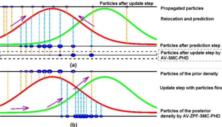
The AV-SMC-PHD filter, however, suffers from the weight degeneracy problem, as illustrated in Fig. 1(a), where ten particles are shown in blue solid circles, with their weights indicated by the size of the circles, and the prior density and the likelihood as the red and green solid lines, respectively. At the top of the figure, the propagated particles are given. After the relocation step, most of the particles converge to the
area around the peak of the prior density. In the prediction step, the weights of the particles are adjusted. According to the Bayes’ theorem, the posterior density is proportional to the multiplication of the prior density with the likelihood density, and its estimation becomes less accurate when no particles are around the posterior density. As a result, only a small number of particles have high weights after the update step.
In addition, the color histograms of the speakers’ faces were used as measurements for particle update. The weights of the particles may decrease sharply when the speakers do not face the camera, and this can lead to unreliable tracking results.
Finally, the particles are relocated based on the DOA lines via Eq. (13) and Eq. (14), and thus they could be migrated from the undetected speaker to the clutter or other speakers, when the DOA estimation is corrupted by background clutter.
Fig. 1: Illustration of (a) the weight degeneracy problem and (b) the particle flow process. The particles are shown as the blue circles whose sizes indicate their weights. The prior density and likelihood density are represented by the red dashed and green solid lines, respectively.
III. PROPOSEDAVPARTICLE FLOWSMC-PHD FILTER To address the above problems, we propose an AV particle flow SMC-PHD filter, where the particle flow is used for particle migration before the update step of the AV-SMC-PHD filter (i.e. Step 4 of Algorithm 1). Furthermore, the measurementszr
k used in particle flow Eq. (9) and update step
Eq. (5) are replaced by the candidate speaker states, calculated in terms of DOA and color histograms. The speaker states in the previous frames are also used to relocate surviving particles with DOA at Step 2 of Algorithm 1. This allows performance benchmarking with the baseline method in [5], to show the advantage of our proposed method. However, to show the flexibility of the proposed method, we have also considered other type of visual measurements such as those obtained by a state-of-the-art deep learning based face detector, in our experiments.
A. Particle flow for AV-SMC-PHD filter
We consider both ZPF and NPF in our proposed algorithms. As the number of speakers and the labels of the particles are unknown and time-varying, we assume that the number of
particle flows is identical to the number of candidate speakers ˜
Nk|k−1. The particles are clustered for the particle flow based
on candidate speaker states m˜jk|k−1, as discussed in Section III-B. However, in practice, some particles are created due to clutter and noise. We assume that each flow will only be influenced by the particles in the neighborhood of m˜jk|k−1 within certain distance ξf,
m i k|k−1−m˜ j k|k−1 2< ξf (15)
The flow will be applied to the set of particles, {mik|k−1, ωki|k−1}i∈Λ( ˜mj
k|k−1)
, where Λ( ˜mjk|k−1)is a subset of [1,· · ·, Nk], determined via (15), in terms of the threshold
ξf. A high ξf may lead to an inaccurate estimation of the
variance of the speaker states, while a low ξf may result in
an insufficient number of particles for estimating the variance of the target state. In practice, ξf is set according to the
variance of the measurement noise, estimated empirically in our experiments. The mean state m¯k|k−1 of this particle set
is given by: ¯ mk|k−1= P i∈Λ( ˜mjk|k−1) ωki|k−1Fm mik−1 P i∈Λ( ˜mjk|k−1)ω i k|k−1 (16)
The covariance matrix Pk|k−1of this particle set is given by:
Pk|k−1= P i∈Λ( ˜mjk|k−1) ωi k|k−1e(m i k−1)e(m i k−1) T P i∈Λ( ˜mjk|k−1)ω i k|k−1 (17) where e(mik−1) =Fm mik−1 −m¯k|k−1 (18)
For the ith particle in the subset Λ( ˜mjk|k−1), Pi
k|k−1 and
¯
mi
k|k−1in Eq. (8) and Eq. (9) are set asPk|k−1andm¯k|k−1,
respectively.
1) Zero Diffusion Particle Flow: For ZPF, the particle flow is calculated by Eqs. (7)-(10) and the measurement modelHi k
for the ith particle is calculated as,
Hki = ∂Fz(m i k,ςk) ∂mi k mi k|k−1 (19)
In this paper, as the measurement is replaced by the candidate speaker state, Hki ∈R4×4 is taken as an identity matrix.
The flow fi
k,λ of the particle set {mik|k−1}i∈Λ( ˜mjk|k−1) is
calculated via Eq. (7) and applied for migrating the particles.
Ai
k and bik are derived according to Eq. (8) and Eq. (9).
Since the particle states have been updated, the weights of {mik|k−1}i∈Λ( ˜mj
k|k−1)
may have a poor representation of the prior distribution. As the weights are inversely proportional to the proposal distribution as Eq. (3), the weights should be adjusted by: ωik|k−1⇐ qk(m i k|k−1|m˜ j k|k−1)|det(I+ ∆λA i k(λ))| qk(mik|k−1+4λfk,λi |m˜ j k|k−1) ωki|k−1 (20)
where the proposal distribution qk(mik|k−1|m˜
j
k|k−1) ∝
N( ˜mjk|k−1,Σ2
q), Σq is the covariance of the proposal
dis-tribution [66], [67], and det is a determinant.4λis the step of the pseudo time, and the choice of this parameter dictates a trade-off between the computational cost for calculating the particle flow, and the accuracy for estimating the posterior probability. Although det(I+ ∆λAi
k(λ))is a constant for the
particles in the same set Λ( ˜mjk|k−1), it may be different for particles in different set Λ( ˜mjk|k−1) and thus improves the estimate of the particle weights [43].
2) Non-zero Diffusion Particle Flow: For NPF, the particle flowfi
k,λis calculated by Eqs. (11)-(12), where ∇loghikand
∇2loghi k are calculated as ∇loghik =∇h i k hi k (21) ∇2loghi k= ∇2hi k hi k −(∇loghik)(∇loghik)T (22)
Whenhikis Gaussian, we have∇loghik =Pk−|k1−1(mik|k−1− ¯
mk|k−1)and∇2loghik =P
−1
k|k−1[45]. The weight is adjusted
by: ωik|k−1⇐ qk(m i k|k−1|m˜ j k|k−1)|det(I+∇f i k,λ)| qk(mik|k−1+4λfk,λi |m˜jk|k−1) ωki|k−1 (23) where ∇fk,λi = fi k,λ−fk,λi −4λ 4λfi k,λ λ6= 0 0 λ= 0 (24)
The particle statemi
k|k−1 is updated by:
mik|k−1⇐mki|k−1+4λfk,λi (25) The pseudo code of particle flow is given in Algorithm 2, where {m˜jk|k−1}N˜k|k−1
j=1 is the candidate speaker state which
replaces zrk in Eq. (9). After applying Algorithm 2, ωik|k−1
will be updated to ωik by Eq. (5). The particle flow step is also illustrated in Fig. 1(b). The particles are moved towards the peak of the likelihood. As a result, most of the particles are localized between the two peaks of the prior density (red line) and the likelihood density (green line). This means that the shifted particles provide an improved local characterization of the posterior density.
B. Candidate Speaker States
In this subsection, we explain how the candidate speaker states are estimated using audio-visual information e.g. DOA and color histograms. It is worth noting that our proposed tracking framework is flexible and can be adapted easily to accommodate other audio-visual information, such as face detector [10], as considered in our experiments. The DOA information can be obtained by either a circular array (as in our work) or a linear array. As the DOAs are determined by the relative delay between the pairs of microphone signals [5], it only shows the approximate direction θok of the sound sources with respect to the microphones. In practice, the
Algorithm 2 Particle flow for the AV-SMC-PHD filter Input:{mi k|k−1, ω i k|k−1} Nk i=1 and{m˜ j k|k−1} ˜ Nk|k−1 j=1 . Output: {mik|k−1, ωik|k−1}Nk i=1. Initialize: ξf,4λ,Nλ,R,e,Fz,ςk andΣq. Run: foreach m˜jk|k−1 do
Select particle set Λ( ˜mjk|k−1)according to Eq. (15). Calculate m¯k|k−1andPk|k−1 by (16) and Eq. (17),
respectively. Set m¯i
k|k−1= ¯mk|k−1 andPki|k−1=Pk|k−1. fori∈Λ( ˜mjk|k−1)do
forλ∈[0,4λ,24λ,· · · , Nλ4λ] do
if Zero diffusion particle flowthen
Evaluate flow fi
k,λ by Eqs. (7)-(10).
Update the particle weights by Eq. (20).
if Non-zero diffusion particle flowthen
Evaluate flow fi
k,λ by Eqs. (11)-(12).
Update the particle weights by Eq. (23). Update mik|k−1 by Eq. (25).
rectangular coordinate [xo
k, yko] of m˚ok can be transformed to
polar coordinate [ro
k, θko], where rok is the Euclidean distance
from the nearby speaker state at the previous frame to the microphone position, rok= [˜x ˆ j k−1,y˜ ˆ j k−1] T−[x mic, ymic]T 2 (26) where ˆ j= argmin j ˜
yjk−1−ymic−(˜xjk−1−xmic) tanθko
˜
xjk−1−xmic−(˜yjk−1−ymic) tanθko
1 (27)
where k.k1 and k.k2 are the L1 and L2 norm, respectively.
[˜xjk−1,y˜jk−1]T and[x
mic, ymic]T are the positions of the jth
speaker state at the previous frame m˜jk−1 and the state of microphone array mmic, respectively. They both correspond
to the center of the microphone array. Here, the aim is to find the index of the speaker, i.e. ˆj, which gives the minimum tangent value of the angle between the DOA θko and the direction of each target speaker. Then m˚ok is given by:
˚
mok = [rokcosθko+xmic, rkosinθ o k+ymic,0,0]T (28) The weight˚ωo k ofm˚ok is given by, ˚ωko=N(θok|arcsin(y˜ j k−1−ymic ro k ), σo2) (29) whereσ2
o is the variance of the DOA angle distribution. The
candidate speaker states{m˜jk|k−1}N˜k|k−1
j=1 can be calculated as ˜ mjk|k−1= (˚ωˆo km˚okˆ+ ˘ωkum˘uk ˚ωˆo k+ ˘ω u k , ifdu,ˆo m ≤ξm ˘ muk, ifdu,mˆo> ξm (30) where du,moˆ= [˚xˆok,˚ykˆo]T−[˘xuk,y˘uk]T 2 (31) where ω˘u
k is the weight for m˘ u
k, which can be obtained by
CAMShift [9] or face detector [10].[˘xu k,y˘
u k]
T is the position
information taken fromm˘u
k. As the association betweenm˚okˆ
andm˘u
k is unknown and time-varying, we assumeN˜k|k−1 is
equal to the number of the speakers detected, and o is the index of the DOA line that is closest to m˘u
k. ˆ o= argmin o du,om (32) In practice,m˚ˆo kandm˘ u
k may represent different speaker states.
To address this issue, the distance du,oˆ
m is compared with a
threshold value ξm. If du,moˆ ≤ ξm, m˜
j
k|k−1 is estimated in
terms of the DOA and color histograms. When the speakers go out of the view of the camera or are visually occluded,mu k
will become inaccurate. In this case, the DOA lines near the speaker will be used to calculate the candidate speaker states which are then used to calculate the likelihood as:
hi,jk ∝ N( ˜mik|k−1−m˜jk|k−1|0,Σh) (33)
whereΣh is the covariance of the likelihood andhi,rk in Eq.
(5) is replaced by hi,jk . As a result, the particle weights are likely to retain high values even when the speakers do not face the camera. If du,ˆo
m > ξm, m˜
j
k|k−1 is only estimated by the
uth color histograms.
The pseudo code for calculating the candidate speaker state is given in Algorithm 3, which, together with Algorithm 2, can be plugged into Step 4 of Algorithm 1.
Algorithm 3 Candidate Speaker States
Input: DOA lines, reference color histograms, {m˜jk−1}N˜k−1 j=1 and{m i k|k−1, ω i k|k−1} Nk i=1. Output: {m˜jk|k−1}N˜k|k−1 j=1 . Initialize: mmic,ξm andσo.
Run:
foreach DOA line indexed byo do
Calculate θok from the DOA line [5].
Select the nearby speakerm˜ˆjk−1 as Eq. (27).
Calculaterokand˚ωokas Eq. (26) and Eq. (29), respectively. Calculate m˚ok as Eq. (28).
j= 0
foreach reference histogram indexed by udo
iftheuth reference histogram is detectedthenj=j+ 1. Calculatem˘uk andω˘ku by CAMShift [9].
Select the nearbym˚okˆ as Eq. (32). Calculatem˜jk|k−1 as Eq. (30). ˜
Nk|k−1=j.
C. Relocating particles
Due to the presence of noise and clutter in acoustic measure-ments, the DOAs estimated are not always reliable. To address this issue, we also consider the speaker state{m˜jk−1}N˜k−1
j=1 at
After calculating di
k by using Eq. (13), the movement
distance di k is updated as dik⇐ (1−ω˜ˆjk)dik+ ˜ωkˆj 4m˜ i k|k−1 2 d i k≤ξd ˜ ωˆkj 4m˜ i k|k−1 2 d i k> ξd (34) where 4m˜ik|k−1=Fm˜( ˜m ˆj k−1,τk)−mik|k−1 (35) ˆj= argmin j Fm˜( ˜m j k−1,τk)−mik|k−1 2 (36)
where ˆj ∈ {1, ...,N˜k−1} is the index of the speaker closest
to the ith particle. The threshold ξd is used to control the
movement distancedi
k, in order to reduce the effect of noise in
DOA estimate. When the DOA estimates are noisy, we relocate the particles in terms of the motion model, otherwise, in terms of the DOA and the speaker states in the previous frames. In our work, ξd is set empirically according to the variance of
the DOA estimates. As the particles are located near the DOA lines, the relocation step is applied only when Uk 6= ˜Nk−1,
where UkandN˜k−1are the number of audio measurements at
timekand the number of speakers at timek−1, respectively. The DOAs are also applied to detect new speakers, i.e. whether Step 2 in Algorithm 1 is needed. Comparing the number of visual measurements Ok with N˜k−1, the PHD
filter is able to identify the appearance and disappearance of speakers. If Ok = ˜Nk−1, the number of speakers remains
unchanged. IfOk<N˜k−1, the speakers may walk out of the
camera view, or be occluded by other speakers. IfOk >N˜k−1,
new speakers may appear in the scene, and hence new born particles are created.
IV. EXPERIMENTALEVALUATIONS
The proposed algorithms are evaluated using real AV data. First, we briefly discuss the datasets, baseline algorithms, performance metrics and the parameter set up. Then we show the improvement achieved by the particle flow, the candidate speaker states and the novel localization method. Finally, we compare the proposed methods with several recent baselines.
A. Datasets and Baselines
Several audio-visual datasets are publicly available, such as the AV16.3 [46], AVDIAR [47], AVTRACK-1 [68], AVASM [69], AMI [70], CLEAR [48], MVAD [71] and SPEVI [72]. We have considered our requirements when choosing the datasets. For example, the calibration information should be provided for the projection of the audio information from the physical space to the image plane. In addition, the dataset should contain some challenging situations, e.g, the number of speakers changes and some speakers are occluded. For these reasons, we have chosen AV16.3, AVDIAR and CLEAR datasets in our evaluations.
The AV16.3 [46] consists of real-world data with both audio and video sequences. It provides the calibration information of the cameras to map the audio information from the physical space to the image plane. AV16.3 includes the occlusion as a challenging scenario, and consists of sequences where the
speakers are walking and speaking at the same time. The video and audio signals are recorded by three calibrated video cameras at 25 Hz and two circular eight-element microphone arrays at 16 kHz, respectively. The audio and video streams are synchronized before running the algorithms. The size of each image frame is288×360. All algorithms are tested with all three different camera angles of five sequences: Sequences 1, 24, 25, 30 and 45, which correspond to the cases of one to three speakers and are the most challenging sequences in term of movements of the speakers and occlusions.
Different from the AV16.3 dataset, the speakers in the AVDIAR dataset [47] talk one by one. There are six micro-phones mounted on Sennheiser Triaxial MKE 2002. Two of them are on the left and right ears and the other four are on each side of the head. However, since the details of the microphone positions are not provided, only the microphones on the left and right ears are considered. Another issue is that the calibration information of the cameras is not available. The AVDIAR provides training data to learn a mapping as in [47]. This dataset includes 23 sequences. Each image frame is of 1920×1200pixels. The audio and video were recorded at 48 kHz and 25 Hz, respectively, which were synchronized by an external trigger controlled by software. There are 12 different participants and up to 4 people are recorded in each sequence. AVTRACK-1 [68] and AVASM [69] are provided by the same institution as for AVDIAR. However, they are less chal-lenging than AVDIAR. AMI and MVAD, which are designed for speaker diarization, are not used in our tests since the speakers are mostly static or with small movements. In SPEVI [72], audio signals were recorded with linear microphone ar-rays. Since the calibration information and training set are not available, this dataset is also not chosen. The CLEAR dataset is chosen for our experiments since it has the largest number of speakers among these datasets. Although our proposed algorithms could be used in other scenarios such as sport-video analysis and smart surveillance systems, due to the lack of suitable datasets, such scenarios are not considered here.
Several baselines are considered for benchmarking our proposed algorithms, including AV-PF-PF [43], AV-ZPF-GPF-PHD [29], SAVMS-SMC-AV-ZPF-GPF-PHD [5], auxiliary SMC-AV-ZPF-GPF-PHD filter [23], baseline AV-SMC-PHD filter [5] and the filter proposed in our previous work [7]. For convenience, the AV-ZPF-SMC-PHD, AV-NPF-SMC-AV-ZPF-SMC-PHD, SAVMS-SMC-AV-ZPF-SMC-PHD, AV-PF-PF, AV-ZPF-GPF-PHD, AV-PHD and AV auxiliary SMC-PHD filters are abbreviated as ZPF, NPF, SMS, PPF, GPF, SMC and ASMC respectively. The GLMB method [19] was not considered since it was used only for audio tracking, and did not address the weight degeneracy problem.
B. Performance metrics
We use the Optimal Sub-pattern Assignment (OSPA), ESS, and distance between particles and ground truth speak state as performance metrics.
The OSPA [73] is defined as, OSPA({m˜jk}N˜k j=1,{m˜ ˜ j k} ˜ Nk ˜ j=1) = a v u u u u u t min π∈ΠN˜k ,Nk˜ ˜ Nk X j=1 d(c)( ˜mjk,m˜kπ(j))a+ca( ˜Nk−N˜k) ˜ Nk (37) where{m˜1k, ...,m˜N˜k
k }is the set of ground truth speaker states,
and{m˜1
k, ...,m˜
˜
Nk
k }is the set of the estimated speaker states.
ΠN˜
k,N˜k is the set of maps π : 1, ...,
˜
Nk → 1, ...,N˜k. Here
the state cardinality estimation N˜k may not be the same as
the ground truthN˜k. The OSPA error given in Eq. (37) is for
˜ Nk ≤N˜k. IfN˜k<N˜k, then OSPA({m˜ j k} ˜ Nk j=1),{m˜ ˜ j k} ˜ Nk ˜ j=1) = OSPA({m˜˜jk}N˜k ˜ j=1,{m˜ j k} ˜ Nk
j=1)). The functiond¯(c)(·)is defined
as min(c,d(·))¯ wherec is the cut-off value, which determines the relative weighting of the penalties for the cardinality and localization errors andais the metric order which determines the sensitivity to outliers. A lower OSPA implies a better performance.
ESS is applied widely to evaluate the severity of weight degeneracy problem [43], [20], [32], which is given by
ESS= ( PNk i=1ω i k) 2 PNk i=1(ω i k)2 (38) When ESS is small, e.g. ESS < Nk/2, the resampling step
is performed with the uniform weights. When ESS is high, more particles are used to estimate the posterior density with an increased accuracy.
As the label information for each particle is unavailable, the minimal distancedm(mik|k−1)between each particle and
speaker is used: dm(mik|k−1) =˜min j∈Nk m i k|k−1−m˜ ˜j k−1 2 (39) C. Parameter settings
In this subsection, we discuss the setting of five important parameters, i.e. pseudo timeλ, the number of particlesNk, and
three thresholdsξf,ξm, andξd. We only show the experiments
based on ZPF, as these are similar to NPF. Other parameters are given as in the baseline method SMC [5]. The parameters used for detecting the DOAs are set the same as in [74]. The initial distributions of the particles are randomly sampled in the tracking area. If the particles move out of the tracking area, we will reject and resample them. Resampling is performed when ESS is smaller than N/2. The order parameter a in OSPA is set to 2. These parameters are chosen empirically based on our earlier studies [7], [20]. All experiments are run on a computer with Intel i7-3770 CPU with a clock frequency of 3.40 GHz and 8G RAM. Each experiment is repeated 50 times, and the average results are presented.
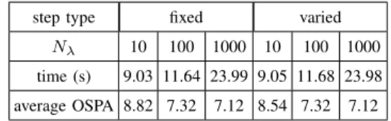
1) Pseudo time: The pseudo time λ in the particle flow is increased incrementally from 0 to 1, with a step size ∆λ, which is either fixed as in [75] or varied as in [43], [32]. Six situations are considered. Here, we have tested three fixed step sizes, i.e. ∆λ= 0.1, 0.01 and 0.001, and three varied:
∆λ= 0.0385×1.2λ×Nλ,2.4×10−9×1.2λ×Nλ, and1.3×
10−80×1.2λ×Nλ. In both cases, the number of steps N
λ is
chosen as 10, 100, 1000, respectively. Sequence 01 (camera 1) from the AV16.3 dataset is used since there is only one speaker and it is easy to see the impact of different pseudo times.
TABLE II: Running time (s) and tracking accuracy in OSPA of ZPF versusλsteps.
step type fixed varied
Nλ 10 100 1000 10 100 1000
time (s) 9.03 11.64 23.99 9.05 11.68 23.98 average OSPA 8.82 7.32 7.12 8.54 7.32 7.12
Table II shows the running time and OSPA of ZPF versus the step type and Nλ. It can be seen that a smaller step size
leads to a smaller OSPA but with a longer running time. For the case of Nλ = 100 with a fixed time step size, a
good balance between OSPA at about 7.3 and running time at about 11.6s is achieved, therefore, this is used later in our experiments.
2) Number of particles Nk: A large Nk can alleviate the
weight degeneracy problem [76], but induce extra computa-tional cost. Here Nk is set from 10 to 1000. Sequence 01
(camera 1) of the AV16.3 dataset is used. During the iterations of the algorithm, if Nk is greater than a preset value, the
particles with low weights are removed from the particle set. IfNk is smaller than the preset value, the particles with high
weights are duplicated and added into the particle set. The results are shown in Table III. It can be seen that with the increase in the number of particles, OSPA is reduced while the computational cost is increased. When Nk is larger than
50, the OSPA becomes stabilized at approximately 7 and the further improvement is small. For example, compared to the caseNk = 50, usingNk = 500, an OPSA of only 3.1% lower
was achieved, at a cost of nearly ten times computational load. If Nk is smaller than 50, e.g. Nk = 10, OSPA is 37.0471,
implying a higher tracking errors. Therefore,Nk= 50is used
later in our experiments.
TABLE III: Running time (s) and OSPA of ZPF versus the number of particles.
Nk 10 50 100 500 1000
time (s) 2.51 11.63 22.25 111.95 245.40 average OSPA 37.05 7.32 7.22 7.09 6.84
3) Thresholdsξf,ξm, andξd: The parametersξf,ξm, and
ξdare used, respectively, to guide the selection of particles into
Λ( ˜mjk|k−1), to obtain the states for the candidate speakers, and to relocate the particles in the relocation steps. We have tested different values for these parameters ranging from 1 to 288 (for the image height at 288). Since these thresholds were used for different purposes, we have chosen different sequences and frames for the tests, i.e. all the frames in Sequence 45 (camera 1) forξf, frames 500-1000 of Sequence 45 (camera 1) forξm,
and frames 280-500 of Sequence 24 (camera 1) forξd, all from
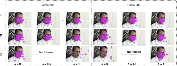
Fig. 2: The motion trails of the particles for the second speaker by NPF, ZPF and SMC. The columns show the results for λ= 0,0.5,1 respectively in the frame 287 and 288 for Sequence 24.
The results are shown in Tables IV. When ξf is increased
to 25, the OSPA is decreased but the running time is increased since more particles are considered in the particle flow. How-ever, with a further increase inξf, the performance in terms of
OSPA starts to degrade, because the particles of the different speakers may be selected into the same set Λ. Whenξm is
increased, OSPA is first decreased from 38.6 to 34.8 and then remains stable. When ξd is increased, the OSPA is decreased
from 22.3 to 20.8 and then remains almost unchanged at 20.8. Therefore, for the AV16.3 dataset, we set ξf, ξm, and ξd
empirically as 25 in our experiments. Note that the running time of our proposed algorithm is not dependent on ξm and
ξd, since only the DOA lines near the particles are considered.
TABLE IV: Running time (s) and OSPA of ZPF versus ξf,
ξm andξd. 1 10 25 50 100 288 ξf 96 286 348 394 493 673 time (s) 26.5 23.8 19.3 24.8 28.5 36.5 OSPA ξm 146 146 146 146 146 146 time (s) 38.6 34.8 31.6 31.6 31.6 31.6 OSPA ξd 52.1 52.1 52.1 52.1 52.1 52.1 time (s) 22.3 21.5 20.8 20.8 20.8 20.8 OSPA
D. Comparison with the baseline methods
In this subsection, we show the improvement achieved by the particle flow, the novel relocation method and the candidate speaker state. First, we compare between particle flows and SMC. Second, we compare particle flows with candidate speaker state and color histograms, respectively. Each speaker is calculated by 50 particles. Third, we compare between our proposed relocation method with the relocation method in SMC [5]. When a new speaker is detected, 50 particles are created and added into the PHD filter. The parameters for the particle flow are set empirically, i.e. 4λ= 0.01and Nλ= 100.
1) Particle flow for weight degeneracy problem: To evalu-ate the particle flow, ZPF, NPF and SMC are compared. Firstly, we only update the particle states by SMC in the frames 270-286 for Sequence 24 on camera 1. In the frames 0-270, there is no speaker or only one speaker, and the weight degeneracy issue does not usually occur. Therefore, these frames are not used for demonstrating the weight degeneracy effect. Note, however, that we have included the results for all the frames in Section IV-E, with a varying number of speakers from 0 to 3. Until frame 286, there are two speakers and most of the particles can track the speakers. In frame 287, the ESS of SMC is smaller thanNk/2 and SMC is encountered
with the weight degeneracy problem. Then this particle set is separately updated by ZPF, NPF and the baseline SMC. In these filters, the candidate speaker state is used. In SMC, we assumehi,jk ∝ N(mik|k−1−m˜jk|k−1,R).hi,rk andzkr in Eq. (5) are replaced byhi,jk andm˜jk|k−1. ESS is calculated at each pseudo time step.
0 0.5 1 Pseudo time 10 20 30 40 50 60 ESS SMC ZPF NPF N k/2 (a) 0 0.5 1 Pseudo time 10 15 20 25 30 OSPA SMC ZPF NPF (b)
Fig. 3: The ESS and OSPA of ZPF, NPF and SMC in the frame 287 of Sequence 24 (camera 1) changes with respect to λ.
Fig. 2 shows how the particles are modified by these filters from λ= 0 to λ= 1. As an example, the first, second and third rows, show the tracking results of NPF, ZPF, and SMC, respectively, for frames 287 and 288. The green lines show
the motion trails of the particles. Note, the face images were actually cropped manually from the video signal to visualize the distribution of the particles around the face area, which is very small in the whole image plane. For NPF and ZPF, three figures are shown for λ = 0,0.5 and 1, respectively. SMC at the third row is shown as the baseline method, where only the predicted and updated results are shown as there is no particle flow step in this filter. Compared to SMC, NPF and ZPF give more accurate estimates for the speaker states. Before resampling, SMC has only four particles located on the speaker’s face and the speaker in frame 287 is not well tracked.
In Fig. 3(a), we show the variation of ESS of NPF, ZPF and SMC fromλ= 0toλ= 1. As the baseline SMC does not use the particle flow, its ESS only has values at the beginning and end of the update step, as shown by the green dashed line. At the beginning of the update step, the ESS of the three filters is about 45, which is lower thanNk/2, shown in the pink
dash-dot line. Using NPF and ZPF, the ESS is increased to 57 and 58, respectively, and therefore the particles do not need to be resampled. When λ <0.5, the improvement of ESS given by NPF is higher than that given by ZPF. In Fig. 3(b), the OSPAs of the three filters are shown at eachλ. After the update step, the OSPAs of NPF and ZPF are both decreased to 12. This shows that ZPF and NPF provide more accurate estimate of the speaker state than SMC. When λ = 0.95, the OSPA of ZPF increases slightly, due to the measurement errors. Fig. 4 shows the average OSPA and the number of speakers for the frames 287-500. It can be observed that ZPF and NPF give a smaller average OSPA than SMC. Due to the presence of occlusion from frames 300 to 500, the OSPAs for all methods have increased. At frame 345, ZPF and NPF give an average OSPA at about 19.3 and 18.9, respectively, resulting in a 24% and 29% performance improvement over SMC thanks to the more accurate estimate of the number of speakers offered by the particle flow.
300 350 400 450 500 Pseudo time 10 20 30 OSPA (pixel) SMC ZPF NPF 300 350 400 450 500 Pseudo time 0.5 1 1.5 2 2.5 No. of speakers True SMC ZPF NPF
Fig. 4: The average OSPA of SMC, ZPF and NPF and the estimated number of speakers in the frames 287-500 of Sequence 24 (camera 1).
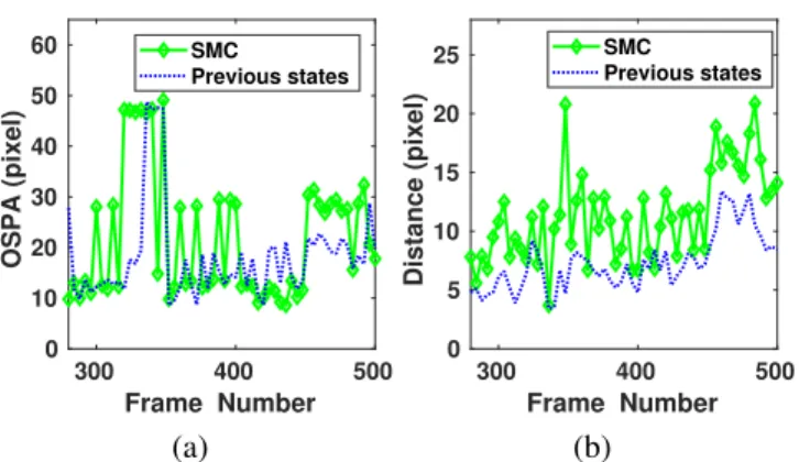
2) Particle relocation methods: Here the baseline SMC and SMC with the novel particle relocation methods are compared. To show the OSPAs of these two filtering algorithms, we
300 400 500 Frame Number 0 10 20 30 40 50 60 OSPA (pixel) SMC Previous states (a) 300 400 500 Frame Number 0 5 10 15 20 25 Distance (pixel) SMC Previous states (b)
Fig. 5: Comparison the OSPA error (a) and the minimal distance dm (b) between the novel relocation method with
the speaker states at the previous time frame and the baseline relocation method of SMC.
ran experiments in frames 280-500 of Sequence 24 camera 1 which involves two speakers and visual occlusion. Fig. 5(a) shows the average OSPA. For convenience, the novel method in which the particles are relocated with the previous speaker states are abbreviated as Previous states. The average OSPA error is 20.8 for the novel method and 22.6 for the baseline method SMC. This means that the novel relocation method offers an 8% improvement over the baseline method.
Apart from that, Fig. 5(b) shows the distance measure in terms of Eq. (39). The average is 6.77 for the novel method and 10.78 for the baseline method. The novel relocation method offers 37% improvements. The running time of the novel relocation step (0.0529s) is higher than that of the baseline method (0.0218s), however, the running time of the overall algorithms are similar.
3) Candidate speaker states: To show the impact of using the candidate speaker states m˜jk|k−1, ZPF is compared with the filter in our earlier work [7]. Although both methods use ZPF, DOA lines are used only in the update step of ZPF, rather than in that of the filter in [7]. Other steps and parameters of these filters are the same. The frames 500-1000 of Sequence 45 are used to test both methods since in these frames the speakers go out of the view of cameras which represents a challenging tracking scenario.
500 600 700 800 900 1000 Frame Number 0 20 40 60 OSPA (pixel) [7] ZPF (a) 500 600 700 800 900 1000 Frame Number 1 2 3 No. of speakers True ZPF [7] (b)
Fig. 6: Comparison of ZPF and the filter in [7] in terms of OSPA and the number of speakers.
Fig. 6(a) shows the average OSPA for this sequence, which is 38.6 for the filter in [7] and 31.6 for ZPF. This means that
TABLE V: The experimental results for NPF, ZPF and SMC with different levels of noise and different number of clutter in terms of the OSPA error
Method σς Nc
0 10 20 30 0 5 10 50
NPF 19.41 23.54 26.71 32.94 19.41 19.75 21.81 24.37 ZPF 19.33 23.55 25.51 31.42 19.33 19.47 20.06 21.86 SMC 29.46 31.52 39.12 39.94 29.46 29.57 30.14 32.07
the proposed relocation method offers 19% improvements over the filter in [7]. In the frames 620-700, the average OSPA error is 21.6 for ZPF, and 38.2 for the filter in [7]. Fig. 6(b) shows that ZPF offers more accurate estimates for the number of speakers than the filter in [7], especially for the frames 620-700. The average running time of ZPF and the filter in [7] are 146.8s and 143.5s, respectively. This means the use of audio information leads to only 2.3% increase in running time.
4) Clutter and noise: We also evaluated the performance of our proposed filter in different levels of clutter and noise, as compared with SMC, using Sequence 45 of the AV16.3 dataset. Fig. 7 shows a frame of sequence 45 with clutter and noise. Gaussian noise ςk ∝ N(0,σς)and random clutter
are added to the visual detection, whereσς is the covariance
matrix of noise. The clutter is shown in green stars. The visual detection without noise is shown in red points and its noise version in yellow diamonds. Table V shows the OSPA for different levels of noise with σς set from 0 to 30 pixels and
the different number of clutter withNc set from 0 to 50. We
observe that particle flow gives a smaller OSPA, as compared with SMC, confirming that particle flow can improve the performance of SMC in different levels of noise. The positions of clutter are randomly set in the tracking area. The OSPA of three filters slightly increases with the level of clutter due to the RFS model used, however, the ZPF and NPF offer 32% and 24% improvement, respectively, even when Nc= 50.
Fig. 7: The clutter and noise in Frame 325 of Sequence 45. The measurements, their noisy versions, and the clutter are shown in red points, yellow diamonds, and green stars, respectively.
5) Comparison with face detector: Here we compare the performance difference for using color histogram versus using measurements obtained by a face detector, e.g. the convolu-tional neural networks (CNNs) based face detector (Tiny) [10].
To distinguish the filters with face detectors from the filters with color histogram, ZPF, PPF, GPF, SMC and NPF with the face detector are renamed as AFZPF, AFPPF, AFGPF, AF-SMC and AFNPF, respectively, where AF means both audio measurements (i.e. DoA) and visual measurements (obtained by face detector) are used in these algorithms. The frames 250-300 and 530-580 of the Sequence 45 camera 1 are used for evaluations since unreliable detection and occlusion happen in these frames. The OSPA and ESS of the different filters are shown in Table VI where ESS is not available for the Tiny face detector. AFZPF offers the lowest OSPA and highest ESS among all the filters except AFPPF, since the number of speakers is given in AFPPF. With the zero-diffusion particle flow, the OSPA of AFZPF is 51% and 12% lower than those of AFSMC and Tiny detector when speakers are occluded. We also tested these filters on frames 350-400 of the Sequence 45 camera 1 where occlusion does not happen. The face detector gives a lower OSPA than the filters with color histogram, while it gives a similar OSPA to AFZPF, i.e. ZPF with face detector. TABLE VI: Experimental results for ZPF, NPF, AFZPF, AFPPF, AFGPF, AFSMC, AFNPF, and Tiny face detector in terms of the OSPA error and ESS for Sequence 45 camera 1.
Frame ZPF NPF AFZPF AFPPF AFGPF AFSMC AFNPF Tiny 250-300 29.4 29.6 21.6 23.8 23.6 24.3 23.7 43.9 OSPA 82 73 86 90 65 34 81 - ESS 530-580 24.6 25.8 20.9 23.2 22.8 26.5 22.7 39.5 OSPA 96 78 98 99 76 45 95 - ESS 350-400 18.7 19.7 17.2 17.5 17.3 17.7 17.3 17.7 OSPA 115 94 117 118 90 52 115 - ESS
E. Comparison with other audio-visual algorithms
In this subsection, the proposed algorithms ZPF and NPF are compared with several baselines, including PPF [43], GPF [29], SMC [5], ASMC [5] and SMS algorithms [5]. Although Gebru et al. [47] also presented an audio-visual Bayesian framework, we did not consider this in our experiments, since it does not apply any particle flow or PHD filter. The same zero diffusion flow is used in PPF and GPF, as in our proposed ZPF.
In the PPF, the number of speakers is given when the parti-cles are created due to the use of the particle filter framework. However, this information is unknown and time varying in our audio-visual tracking problem. Therefore, the following two situations are considered. For the AV16.3 dataset, the speakers utter together and continuously, therefore the number of speakers is the same as the number of estimated DOA lines. For the AVDIAR dataset, as the speakers are talking one by one, the number of speakers is given before running the algorithm. GPF is integrated with zero diffusion flow [29]. Based on the Gaussian mixture model, each particle has one dependent variance. Other parameters are the same as in ZPF. The NPF used is based on [45]. We set 4λ = 0.01 and Nk = 50, as already tested in the experiments shown
in Section IV-C. To allow for fair comparison, the same measurements were used in all the filters compared.
Table VII reports the average OSPA over 50 random tests. All the frames of the 12 sequences have been used in these tests, where the number of speakers is varying with time. It can be observed that, using ZPF and NPF, about 31% reduction in tracking error has been achieved as compared with SMC. Compared with the ASMC filter, ZPF and NPF both give about 20% reduction in OSPA.
TABLE VII: The experimental results for ZPF, SMS, PPF, GPF, SMC, ASMC and NPF in terms of the OSPA error
Seq ZPF SMS PPF GPF SMC ASMC NPF 24(1) 12.35 14.50 12.18 13.00 17.71 14.68 13.32 24(2) 13.24 15.35 13.12 15.13 19.83 16.15 13.20 24(3) 13.15 15.72 13.02 15.22 18.94 15.24 13.23 25(1) 15.94 17.17 14.90 18.28 19.13 16.21 15.96 25(2) 15.21 15.39 13.08 15.58 18.47 15.67 15.29 25(3) 16.22 17.62 14.98 18.62 21.61 17.95 16.29 30(1) 15.82 19.27 15.29 18.89 25.22 22.84 15.76 30(2) 13.43 16.16 13.86 16.12 19.37 16.17 13.41 30(3) 16.01 19.67 15.61 19.03 25.31 21.75 15.93 45(1) 17.60 23.40 24.50 23.12 29.46 26.07 17.65 45(2) 18.55 23.16 22.26 22.71 29.47 25.97 18.60 45(3) 19.54 23.80 24.34 23.76 28.43 26.41 19.50 Avg 15.59 18.43 16.43 18.28 22.75 19.59 15.68
To show how significant the difference is among the results of the tested algorithms in Table VII, the ANOVA based F-test [77] is applied and the significance test results are given in Table VIII. As the degree of freedoms for all the significance tests is (1,22) and the significance value is 5%, the corresponding critical value Fcrit for (1,22) is 4.30 in
terms of the F-distribution table [77] where the F-value is the ratio of the between-group variability to the within-group variability. The p-value is the probability of a more extreme result than the value achieved when the null hypothesis is true. According to the test, the results are considered as statistically significant if F-value > Fcrit and p-value is less than the
significance value (0.05). It can be seen that the improvements of ZPF and NPF, over SMC, SMS and ASMC are statistically significant. However, the difference between ZPF and PPF is not significant. Nonetheless, in ZPF, the number of speakers is estimated, while in PPF, this is given as prior information. The difference between ZPF and NPF is also not significant. TABLE VIII: Significance test for ZPF, SMS, PPF, GPF, ASMC and NPF. Method ZPF SMS PPF GPF ASMC NPF ZPF - 5.84 0.33 5.10 7.14 0.01 F - 0.024 0.057 0.034 0.014 0.921 p-value NPF 0.01 5.64 0.027 4.89 6.98 - F 0.921 0.027 0.610 0.038 0.015 - p-value SMC 23.84 6.92 11.6 7.27 2.8 23.7 F
7e-07 0.015 0.003 0.013 0.1082 7e-05 p-value
As shown in Table IX, ZPF has a lower computational cost than GPF. Although ZPF and GPF use the same initial number of particles, the number of particles is drastically varying and a few particles are added in the update step of the GPF. For further understanding, we calculated the total number of particles used in the update step of ZPF and GPF. In the update step of ZPF, the average number of particles is 108, while in GPF, it is 463. The computational complexities are shown in the last line of Table IX. The complexity (Com) of SMC, SMC and ASMC is the lowest atUkNk. The complexity of ZPF, PPF
and NPF does not depend on the number of measurements.
TABLE IX: Computational cost comparison per Sequence (s/Sequence) for ZPF, SMS, PPF, GPF, ASMC and NPF.
Seq ZPF SMS PPF GPF SMC ASMC NPF 24 234.5 146.2 211.3 435.3 80.6 102.5 174.6 25 236.0 147.2 210.6 435.5 83.6 105.2 175.7 30 235.1 146.8 211.7 436.8 83.7 105.4 174.9 45 347.8 208.5 315.9 655.3 124.3 172.9 264.6 Time 263.4 162.2 237.4 490.7 93.1 121.5 197.5 Com NkNλ UkNk NkNλ UkNkNλ UkNk UkNk NkNλ
To show the performance of the proposed method on other datasets rather than AV16.3, we selected sequence 32 (four speakers) and 09 (three speakers) from the AVDIAR dataset [47], and the frames 100-170 (four speakers) and frames 180-250 (five speakers) of sequence UKA from the CLEAR dataset [48]. Their average errors are summarised in Table X. Our proposed ZPF and NPF methods offer a similar OSPA which is the lowest OSPA among all the filters except PPF. Note that the number of speakers is given to PPF as a priori. However, as the speakers are talking one by one, the performance difference among the compared filters is not significant. The OSPA of all the methods is increased with the increase in the number of speakers.
TABLE X: Experimental results for ZPF, SMS, PPF, GPF, SMC and NPF in terms of the OSPA error for Sequence 09 and 32 of the AVDIAR dataset and frames 100-170 and frames 180-250 of sequence UKA 20060726 of the CLEAR dataset.
Filters sequence 09 sequence 32 frames 100-170 frames 180-250
ZPF 13.72 14.37 28.62 31.57 SMS 13.95 14.90 29.35 36.68 PPF 11.68 12.14 24.21 26.65 GPF 13.82 14.78 30.25 37.84 SMC 14.96 16.86 31.58 38.61 NPF 13.80 14.42 28.60 31.55 V. CONCLUSION
We have presented a new method for mitigating the particle degeneracy issue in SMC-PHD filtering, and implemented both the zero-flow and non-zero flow algorithms for audio-visual multi-speaker tracking. We have demonstrated the ad-vantages of the proposed algorithms as compared with several