Topics on Estimation, Prediction and Bounding Risk for Multivariate Extremes.

(1)

Topics on estimation, prediction and bounding risk

for multivariate extremes

by

Robert Alohimakalani Yuen

A dissertation submitted in partial fulfillment of the requirements for the degree of

Doctor of Philosophy (Statistics)

in The University of Michigan 2015

Doctoral Committee:

Associate Professor Stilian A. Stoev, Chair Assistant Professor Veronica Berrocal Professor Tailen Hsing

(2)

Ma ka hana ka ‘ike

(3)

c

(4)

(5)

ACKNOWLEDGEMENTS

I first want to thank my advisor Stilian Stoev for his encouragement, shrewd advice and most of all his validation of my academic per suits. I also warmly thank professors Tailen Hsing, Kerby Shedden and Veronica Berrocal for serving on my thesis committee. In particular, I want to thank professor Berrocal for her guidance and advice during my time as a graduate student.

I would like to acknowledge the following people who have all played instrumen-tal roles during my time as a student: Joyce Nielson, Brian Mclain, Amy Bailey, Dan Cooley, Tilmann Gneiting, Yizao Wang , Kim Paxton, Daniel Almiral and Pe-ter Guttorp. Generous funding was provided by the Kamehameha Schools Bishop Estate and the Horace H. Rackham Graduate School. I also want to say a special thanks to Judith McDonald and the administrative staff of the University of Michigan Department of Statistics for all their assistance.

Many thanks to my parents, Dominica, Joseph, Anthony and Linda, my grand-father Robert and my sister Rachel. To my son Kaleo, thank you for teaching me that happiness is anywhere you care look. Finally, I want to thank my wife Shannon for her sacrifice, unwavering support and spirited companionship. She deserves much credit for this work and without her this undertaking would not be possible.

(6)

LIST OF FIGURES

Figure

2.1 Schlather max-stable model realizations using correlation functions of Table 2.1 under varying parameter settings. Top: Stable correlation function. Middle: Mat´ern correlation function. Bottom: Cauchy correlation function. Realizations were generated using theRpackage

SpatialExtremes (Ribatet, 2011). The circles indicate locations of “observation staions” in the simulation study of Section 2.4. . . 16 3.1 Four realizations from the log-Gauss-Pareto process (3.6) with Z ∼

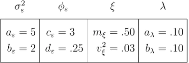
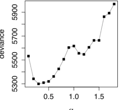
GPD(µ = 0, σ = 1, ξ = 0.5), λ∼ exp(1), ω ∼ uniform(S), and α = 0.5. The process has been censored below 0.1mm. The_N correspond to the process origin ω for each of the four realizations. . . 47 3.2 Map of synoptic stations over south central Sweden. . . 56 3.3 Deviance scores (3.10) of model fit versus smoothness parameter α. 58 3.4 Posterior mean of origin centers ˆωi versus location of maximum

ob-servation smax

i . . . 59

3.5 Distribution of posterior means for the rangeλi and intensitiesZi for

each fitted date i= 1, . . . ,59. . . 60 3.6 Probability integral transform histograms of the predictive

distribu-tions at 21 validation sites . Solid horizontal lines correspond to perfect uniformity. Confidence bands (dashed lines) are provided for reference, bin heights from random draws of a standard uniform dis-tribution should fall outside of the dashed lines in approximately ten percent of cases. . . 61

(9)

4.1 (a) Interpreting β for a 3 asset portfolio: Since β{1} = 0.5, half of

the shocks to asset 1 occur independently from 2 and 3 and since β{1,2,3} = 0.5, the remaining half of the shocks affecting 1 also affect

assets 2 and 3. Similarly, sinceβ{2} = 0.25, one quarter of the shocks

to asset 2 occur independently of 1 and 3; since β{2,3} = 0.25,

an-other quarter of the shocks to asset 2 occur independently of 1 but also affect 3, and since β{1,2,3} = 0.5 the remaining half of the shocks

affecting 2 also affect the entire portfolio. Finally, the sum of all βJk

is equal to the extremal coefficient ϑX({1, . . . , d}) = 1.75. (b)

Pair-wise tail-dependence graph. Edge weights between nodes correspond to bivariate tail dependence coefficients w(i, j) from (4.13). Edge weights at each node indicate level of asymptotic independence β{j}

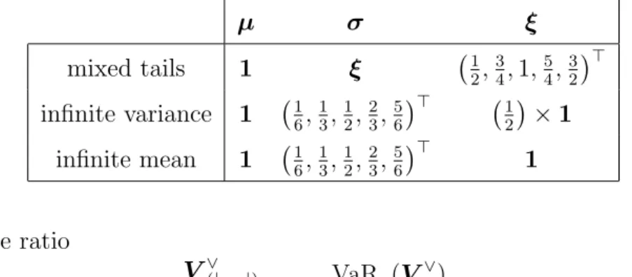
for components j ∈ {1,2,3}. . . 69 4.2 Ratio of Value-at-Risk for component-wise maxima of max-linear

model V versus TM model W = TM(V). Grey lines indicate 100 replicates of the ratio (4.25) and the dark line reports the median. Rows correspond to coefficient matricesA1 andA2in (4.24) for max-linear model (4.23). Columns indicate different values of the shape and scale parameters ξ and σ for the margins of V. . . 79 4.3 TM estimation results for max-linear model A1. Reported are

box-plots of 1000 replicates of fitted TM model coefficients ˆβJk using

sample sizen = 50. The trueβJk for this model are indicated by the

dark points•. The top panel corresponds to lighter tails (ξ = 0.5) vs heavier tails (ξ = 1) in the bottom panel. . . 85 4.4 TM estimation results for max-linear model A2. Reported are

box-plots of 1000 replicates of fitted TM model coefficients ˆβJk using

sample sizen = 50. The trueβJk for this model are indicated by the

dark points•. The top panel corresponds to lighter tails (ξ = 0.5) vs heavier tails (ξ = 1) in the bottom panel. . . 86 4.5 Asset-wise annual maximum of negative daily returns for 5 industry

portfolio. Top: Original scale. Bottom: Fr´echet scale. . . 88 4.6 Illustration of the TM model applied to a 5-dimensional portfolio of

stock market sectors. . . 89 4.7 Backtesting time series for annual block maxima. Solid line

indi-cates maxima {V∨_i}n

i=1 of the 5 industry portfolio in Figure 4.5. Broken lines correspond to the series of estimated VaRα(V∨) at

α∈ {.900, .950, .975, .990}used in the backtest. . . 92 4.8 VaR-max ratios for daily maximaR∨versus scaled TM modelM−ξ∗_W∨

using block size M ∈ {20,60,250}. Grey lines indicate 100 empirical versions of the ratio VaRα(R∨)/VaRα(M−ξ

∗

W∨) and the dark line reports the median. Columns indicate different values of the shape and scale parameters for the margins of W. . . 96

(10)

5.1 Results of two experiments. left: d= 6. right: d = 8. 100 random discrete spectral measures (Htrue) were drawn and ordered along the x-axis according to their value of ρ(Htrue, ξ). Bounds (infH,supH)

correspond to optimization over all spectral measures with identical margins and fixed bivariate extremal coefficients. . . 122 5.2 Upper and lower bounds on extreme VaRρξwhen given a single fixed

(11)

LIST OF TABLES

Table

2.1 Correlation functions for Gaussian random fields. For the Mat´ern covariance function, Bα is the modified Bessel function of the second

kind. . . 15 2.2 Logistic model simulation results using 500 replications of sample size

n = 100 and n = 1000. Reported are bias and root mean squared error (RMSE) for CRPS and MLE estimates. Coverages are based on plug-in estimates of 95% asymptotic confidence intervals. In the case of the CRPS estimates, confidence intervals are based on (2.14) and computed using the expressions from Corollary 2.9. . . 25 2.3 CRPS and MCLE estimates for Schlather model. Reported are bias

and root mean squared error (RMSE) of 500 replications using sample size n∈ {100,1000,5000}. CRPS based confidence intervals forθ0 = (100,1) were calculated using plug-in estimates for the expressions in Corollary 2.9 and resulting 95% coverages are reported. Coverages for MCLE estimates are based on the Godambe information (see Padoan et al., 2010). . . 26 2.4 Simulation results of the four dimensional two factor max-linear model

using 500 replications of sample size n = 5000. We compare the CRPS estimator with the M-estimator (M-est) of Einmahl et al. (2012). Their estimator depends on a threshold parameterκ∈(0, n), thus reported values are favorable ranges based off of the graphs in Figure 5 of Einmahl et al. (2012) which plot bias and root mean squared error (RMSE) over a wide range of κ∈[40,1000]. . . 28 3.1 Specification of hyper-parameters for MCMC. . . 57 4.1 GEV parameter settings for VaR-max simulation studies . . . 78 4.2 Medians and inter-quartile range (IQR), in parentheses, for 1000

marginal GEV parameter estimates fitted to samples of size n = 50 generated from the max-linear model (4.23) with coefficient matrices

A1 and A2 of (4.24). Reported are results for the first component V1 only. Results for the remaining components are nearly identical. . . 84

(12)

4.3 TM model backtesting results for 5 industry portfolio. Empirical coverage rates ( ˆα) and naive binomial standard errors for Monthly, Quarterly and Annual TM bounds on VaR-max. The training length and number of tests are given by m and (n−m) respectively. . . . 93 5.1 VaR informationI(ϑ) for all pairwise extremal coefficients. . . 122 5.2 VaR informationI(ϑ) for a single d-variate extremal coefficient. . . 131

(13)

ABSTRACT

Topics on estimation, prediction and bounding risk for multivariate extremes by

Robert Alohimakalani Yuen

Chair: Stilian A. Stoev

This dissertation consists of results in estimation, prediction and bounding risk for multivariate extremes. Regarding estimation, we establish a consistent and asymptot-ically normal M-estimator that is applicable to a wide variety of max-stable models, i.e. the class of distributions arising as the limit of component-wise maxima. Such processes play a fundamental role in modeling extreme phenomena, but are challeng-ing to work with due to a lack of tractable likelihoods. Our method circumvents intractable likelihoods, working directly with distribution functions of max-stable processes which are readily available or can be approximated in a precise manner. Our second contribution is in the area of prediction for spatial extremes, specifically extreme precipitation. We introduce Gauss-Pareto random fields as a flexible class of models that capture essential non-trivial extremal dependence characteristics, yet remain amenable to standard Bayesian MCMC techniques. We apply Gauss-Pareto processes to spatial prediction of extreme precipitation over Sweden and show that Gauss-Pareto models yield skillful predictions in practice. Lastly we establish uni-versal bounds on the extreme Value-at-Risk of various functionals of portfolio losses. Specifically, the maximum portfolio loss and the sum of tail dependent losses

(14)

un-der given summary measures of tail dependence called extremal coefficients. While extremal coefficients are finite dimensional and consistent estimators are readily ob-tainable, they do not fully characterize tail dependence. Prior to this work, it was not known how extremal coefficients constrain Value-at-Risk for extreme losses. The solution involves solving an optimization problem over an infinite dimensional space of measures. Here we prove that the optimization problem can be reduced to a con-vex optimization problem in finite dimensions and develop algorithms to compute the bounds.

(15)

CHAPTER 1

Introduction

Dependence in the tails of a multivariate distribution can be quite different than the dependence structure near its ‘center’. This phenomena can be observed empir-ically in data from a variety of fields including insurance, finance, and atmospheric sciences. Probability models that do not account for such tail dependence are the-oretically blind of contagion effects present during times of extreme shock. A well known example is the class of Gaussian random vectors which are asymptotically independent unless their distribution is degenerate, i.e. two or more variables are ex-actly co-linear. This has motivated a large body of research in multivariate extreme value theory (MEVT), in order to characterize classes of probability models with non-trivial tail dependence - i.e. multivariate extreme value distributions. While a variety of models have been theoretically established, challenges remain in applications be-cause most often there is a lack tractable likelihoods and conditional distributions are quite challenging to work with (see e.g. Wang and Stoev, 2011; Dombry et al., 2012). These difficulties have hampered statistical inference for multivariate extremes. In particular, estimation and prediction for extreme value processes have remained an open area of research.

This dissertation presents three contributions in the area of statistical inference for multivariate extremes, respectively: estimation, prediction and bounding of risk.

(16)

After an introduction to extreme value theory, Chapter 2 introduces a minimum distance estimator for max-stable models - the class of distributions arising as the limit of component-wise maxima. Chapter 3 describes a method for prediction of spatial processes given nearby observed extremes. Chapter 4 introduces the Tawn-Molchanov model as a method for bounding extreme Value-at-Risk for themaximum of dependent losses. Lastly, Chapter 5 is an extension of concepts from the previous Chapter, providing theoretical bounds on extreme Value-at-Risk for the more common sum of dependent losses under fixed extremal coefficients.

1.1 Univariate Extremes

Letη, η1, η2, . . . be independent, identically distributed random variables. If there exists sequences {an}>0, and {bn} ,n = 1,2, . . . such that

a−_n1{max

i≤n ηi−bn} d

→ζ, asn → ∞, (1.1)

for some non-degenerate random variableζ, then by the classical results of Fisher and Tippett (1928) and Gnedenko (1941),ζmust be generalized extreme value distributed (GEV), which has the three parameter distribution function

Gµ,σ,ξ(z) := exp

n

−(1 +ξ(z−µ)/σ)−₊1/ξo, σ >0, (1.2)

where z+ = max{z,0}, and where µ, σ and ξ are the location, scale and shape pa-rameters. The cases ξ > 0, ξ < 0, and ξ →0 correspond to Fr´echet, reverse Weibull, and Gumbel, distributions respectively. When relation (1.1) holds it is said that η belongs to the max-domain of attraction of ζ, denoted η ∈MDA(ζ). (see, e.g. Ch.3 and 6.3 in Embrechts et al., 1997 for a detailed treatment).

(17)

{cn}>0, and {dn} ,n = 1,2, . . . such that for all n

c−_n1{max

i≤n ζi−dn} d

=ζ, (1.3)

whereζ1, ζ2, . . . are independent copies of ζ. In view of (1.1) - (1.3) we have for large enoughn and z, the approximation

P max i≤n ηi ≤z ≈G1_µ,σ,ξ/n c−_n1{z−dn} ≈Gµ,σ,ξ(z)

for some set of parametersµ, σ, ξ. Hence, the distribution of block maxima maxi≤nηi

can be seen as approximately GEV.

Remark 1.1. More generally, when η1, η2, . . .is a stationary time series satisfying mild dependence conditions (Leadbetter et al., 1983), then extreme values tend to appear in clusters. In this case, the extremal index θ ∈ (0,1] determines the mean cluster size 1/θ and block maxima then follow approximately Gθ

µ,σ,ξ(z).

Alternatively, one can model extremes for η by considering excursions over a high threshold u. In this case ifη ∈ MDA(ζ) with ζ ∼Gµ,σ,ξ, then the following relation

holds

P(η > z+u|η > u)≈ 1−Gµ,σ,ξ(z+u) 1−Gµ,σ,ξ(u)

≈(1 +ξz/˜σ)−₊1/ξ, (1.4) where ˜σ =σ+ξ(u−µ). The distribution function (1 +ξz/˜σ)−₊1/ξ in (1.4) is called the generalized Pareto distribution (GPD) and is the only possible non-degenerate limit of _P(η > z+u|η > u) as u → ∞. Thus the GPD serves as a model for peaks over thresholds, in same melody as the GEV with respect to block maxima.

1.2 Multivariate Extremes

Consider ηi ={ηi(s)}s∈S, i = 1,2, . . . as independent and identically distributed

(18)

model wave-height or pollutant concentration levels at a locations in a spatial region S ⊂ _R2_{, or} _η

i(s)’s may model returns for a fund s in a portfolio S ⊂ N. If one

is interested in extremes, it is natural to consider the asymptotic behavior of the point-wise maxima. Suppose that, for some an(s)>0 and bn(s)∈R, we have

n 1 an(s) max i=1,...,nηi(s)−bn(s) o s∈S f.d.d. → {ζ(s)}s∈S, asn → ∞, (1.5)

for some non-trivial limit process ζ, where f.d.d.→ denotes convergence of the finite-dimensional distributions. As with the univariate case, whenever (1.5) holds, we denote η ∈ MDA(ζ). The class of extreme value processes ζ = {ζ(s)}s∈S arising in

the limit describe the statistical dependence of ‘worst case scenaria’ and are therefore natural models of multivariate extremes. The limit ζ in (1.5) is necessarily a max-stable process in the sense that for all n, there exist cn(s) > 0 and dn(s) ∈ R, such that n 1 cn(s) max i=1,...,nζi(s)−dn(s) o s∈S f.d.d. = {ζ(s)}s∈S,

where {ζi(s)}s∈S are independent copies of ζ and where f.d.d.

= means equality of all finite-dimensional distributions. In Section 1.3 we elaborate further on the charac-terization of max-domain of attraction in terms ofmultivariate regular variation (See e.g. Ch.5 of Resnick, 1987).

The dependence structure of the limiting extreme value process ζ rather than its marginals is of utmost interest in practice. Arguably, the type of the marginals is unrelated to the dependence structure of ζ and as it is customarily done, we shall assume that the limit process ζ has been transformed to 1-Fr´echet marginals. That is,

P(ζ(s)≤z) =Gσ(s),σ(s),1(z) =e−σ(s)/z, z >0, (1.6) for some scale σ(s)>0 (Ch.5 of Resnick, 1987).

(19)

Remark 1.2. It is often the case to simplify (1.6) even further and take the marginals of the limit process ζ to bestandard Fr´echet, i.e. _P(ζ(s)≤z) =G1,1,1(z) =e−1/z for alls ∈S. In this case ζ is called simple max-stable (SMS).

Let ζ = {ζ(s)}s∈S be a max-stable process with 1-Fr´echet marginals as in (1.6).

Then, its finite-dimensional distributions are multivariate max-stable random vectors and they have the following representation:

P(ζ(sj)≤zi, i= 1, . . . , d) = exp n − Z Sd+−1 max i=1,...,dui/zi H(du)o, (1.7)

where zj >0, sj ∈S, j = 1, . . . , d and where H =Hs1,...,sd is a finite measure on the

positive unit sphere

Sd+−1 ={u= (uj)dj=1 : uj ≥0, d

X

j=1

uj = 1}

known as the spectral measure of the max-stable random vector (ζ(sj))dj=1 (see e.g. Proposition 5.11 in Resnick, 1987). The integral in the expression (1.7) is referred to as the tail dependence function of the max-stable law. In the following Chapter, we will often use the notation:

σ(z)≡σs1,...,sd(z) := −logP(ζ(sj)≤zi, j = 1, . . . , d),

where z = (sj)dj=1 ∈Rd+, for the tail dependence function of the max-stable random vector (ζ(sj))dj=1.

It readily follows from (1.7) that for all aj ≥ 0, j = 1, . . . , d, the max-linear

combination

max

j=1,...,dajζ(sj), (1.8)

is a 1-Fr´echet random variable with scale R

Sd+−1

(20)

a random vector (ζ(sj))dj=1 with the property that all its non-negative max-linear combinations are 1-Fr´echet is necessarily multivariate max-stable (de Haan, 1978). This invariance to max-linear combinations is an important feature that will be used in our estimation methodology of Chaper 2

Some max-stable models are readily expressed in terms of their spectral measures while others via tail dependence functions. These representations however are not convenient for computer simulation or in the case of random processes, where one needs a handle on all finite-dimensional distributions. The most common construc-tive representation of max-stable process models is based on Poisson point processes (de Haan, 1984; Schlather, 2002; Kabluchko et al., 2009). See also Stoev and Taqqu (2005) for an alternative.

Indeed, consider a measure space (Ω,F, ν) and let Π := {(Γi, Wi)}i∈_Nbe a Poisson

point process on_R+×Ω with intensity measure dΓdν.

Proposition 1.3. Let g :S×Ω7→[0,∞) be ν-integrable for every s∈S and let

ζ(s) := max

i∈N

Γ−_i 1g(s, Wi), s∈S. (1.9)

Then, the process ζ = {ζ(s)}s∈S is max-stable with 1-Fr´echet marginals and

finite-dimensional distributions: P(ζ(sj)≤zj, j = 1, . . . , d) = exp n − Z Ω max j=1,...,dg(sj, w)/zi ν(dw)o. (1.10)

Proof. By (1.9), for all xj >0, j = 1, . . . , d,

P(ζ(sj)≤zj, i= 1, . . . , d) =P(Π⊂A) =P(Π∩Ac =∅),

where

(21)

Observe that Ac ₌_{_{(Γ, w) : max}

j=1,...,dg(sj, w)/zj >Γ}. Since Π is a Poisson point

process on _R+×Ω with intensity dΓν(dw),

P(Π∩Ac=∅) = exp n − Z Ω Z maxj=1,...,dg(sj,w)/zi 0 dΓν(dw)o,

which equals (1.10) and completes the proof. The above argument shows that the integrability of the functionsg(s,·) implies the ζ(sj)’s in (1.9) are non-trivial random

variables.

Relation (1.9) is known as thede Haan spectral representationofζand{g(s,·)}s∈S ⊂

L1

+(Ω,F, ν) as the spectral functions of the process. It can be shown that every sepa-rable in probability max-stable process has such a representation (see de Haan, 1984 and Proposition 3.2 in Stoev and Taqqu, 2005).

Remark 1.4. The expressions (1.7) and (1.10) may be related through a change of variables (Proposition 5.11 Resnick, 1987). While the spectral measure H in (1.7) is unique, a max-stable process has many different spectral function representations. Nevertheless, relation (1.9) provides a constructive and intuitive representation of ζ, that can be used to build interpretable models.

1.3 Regular Variation

A functionF is said to beregularly varying at∞with indexα∈_Rif for allx >0

lim t→∞ F(xt) F(t) =x α .

When α = 0 than we say F is slowly varying. By considering F(x)/xα _{it is always}

possible to write a regularly varying function F as

(22)

where L(x) is a slowly varying function. When studying extremes, regular variation arises in the context of a random variableηhaving regularly varying survival function F(x) = _P(η > x). More precisely, a non-negative random variable η with survival function F(x) is regularly varying if there exists a scalar ξ ∈ _R+ such that for all x >0, lim t→∞ F(xt) F(t) =x −1/ξ_. _(1.11)

In fact, the Pareto tail in (1.11) is the only possible non-degenerate limit of the conditional excess limt→∞P(η > xt|η > t) with x >1 (see e.g. Prop. 2.3 of Resnick, 2007). This, in essence, motivates the regular variation framework for univariate extremes. Since the focus of this dissertation is on multivariate extremes, we will mainly be concerned with a natural extension of (1.11) for random vectors in η = (η(s1), . . . , η(sd)∈Rd+ called multivariate regular variation.

Definition 1.5. A non-negative random vector η ∈ _Rd

+ is multivariate regularly varying if there exists a Radon measure ν on _Rd

+\{0} called the exponent measure such that lim t→∞ P(t−1η ∈[0,x]c) P(t−1η∈[0,1]c) =ν([0,x] c₎ _(1.12) for all x∈_Rd

+\{0}such that [0,x]c is a continuity set ofν.

By Thm 6.1 of Resnick (2007), Definition 1.5 is equivalent to the following spectral measure characterization

Proposition 1.6. Let kηk = η(s1) +· · ·+η(sd). A non-negative random vector η

is multivariate regularly varying if there exists scalars ρ, α >0, a function b(t)→ ∞

and a finite measure H on _Sd₊−1 such that for allx >1

lim t→∞tP kηk> xb(t), η kηk ∈A =ρx−αH(A), (1.13)

(23)

It was shown in Balkema and Resnick (1977) (see also Chap. 5 of Resnick, 1987) that regular variation fully characterizes max-domain of attraction in the sense that Relation (1.12) is necessary and sufficient for η ∈MDA(ζ) where in fact

P(ζ ≤z) = exp{−ν([0,z]c)}.

If the univariate marginals of ζ are normalized to α-Fr´echet, the exponent measure ν, being homogeneous, has the property

ν(tA) =t−αν(A).

Moreover, the limit measure H in (1.13) and the spectral measure of the max-stable

(24)

CHAPTER 2

Minimum distance estimation for max-stable

models

We have seen that max-stable processes form a canonical class of statistical mod-els for multivariate extremes. They appear in a variety of applications ranging from insurance and finance (Embrechts et al., 1997; Finkenst¨adt and Rootz´en, 2004) to spa-tial extremes such as precipitation (Davison and Blanchet, 2011; Davison et al., 2012) and extreme temperature. Recall that max-stable processes are exactly the class of non-degenerate stochastic processes that arise from limits of independent component-wise maxima. However, most max-stable models suffer from intractable likelihoods, thus prohibiting standard maximum likelihood and Bayesian inference. This has motivated development of maximum composite likelihood estimators (MCLE) for max-stable models (Padoan et al., 2010) as well as certain approximate Bayesian approaches (Reich and Shaby, 2012; Erhardt and Smith, 2012).

In contrast to their likelihoods, the cumulative distribution functions (CDFs) for many max-stable models are available in closed form, or they are tractable enough to approximate within arbitrary precision. This motivates statistical inference based on the minimum distance method (Wolfowitz, 1957; Parr and Schucany, 1980). In this Chapter, we propose an M-estimator for parametric max-stable models based on

(25)

minimizing distances of the type Z Rd (Fθ(x)−Fn(x)) 2 ω(dx). (2.1)

whereFθ is ad-dimensional CDF of a parametric model,Fnis a corresponding

empir-ical CDF andω is a weighting measure that emphasizes various regions of the sample space_Rd_._{Using elementary manipulations it can be shown that minimizing distances}

of the type (2.1) is equivalent to minimizing the continuous ranked probability score (CRPS) (Gneiting and Raftery, 2007; Szekely and Rizzo, 2005).

Definition 2.1. (CRPS M-estimator) Let ω be a measure that can be tuned to emphasize regions of a sample space _Rd. Define the CRPS functional

Eθ(x) = Z Rd Fθ(y)−1{x≤y} 2 ω(dy) (2.2)

Then for independent random vectors {Xi}ni=1 with common distribution function Fθ0 we define the following CRPS M-estimator for θ0.

ˆ θn = argmin θ∈Θ n X i=1 Eθ Xi . (2.3)

For simplicity, we shall assume that the parameter space Θ is a compact subset of Rp, for some integer p.

The remainder of this Chapter is organized as follows. In Section 2.1 we introduce several examples of popular max-stable models. In Section 2.2 we establish regularity conditions for consistency and asymptotic normality of the CRPS M-estimator and provide general formulae for calculating its asymptotic covariance matrix. In Section 2.3 we specialize these calculations to the max-stable setting. In Section 2.4 we conduct a simulation study to evaluate the proposed estimator for popular max-stable models.

(26)

2.1 Examples of max-stable models

Recall from (1.9) the spectral representation of a max-stable random field

X(s) := max

i∈_N Γ −1

i g(s, Wi), s∈S, (2.4)

whereg(s,·)∈L1_(Ω,_F_{, ν) and}_{_Γ

i, Wi}∞i=1 are points of a Poisson point process with intensity dΓdν. A great variety of max-stable models can be defined by specifying a measure space (Ω,F, ν) and an accompanying family of spectral functions{g(s,·)}s∈S

or equivalently through a consistent family of spectral measures or tail dependence functions. We review next several popular max-stable models and their basic features.

• (Multivariate logistic) LetX = (Xi)di=1 have the CDF

Fθ(x) = e−σθ(x), where σθ(x) =λ _Xd i=1 x−_i 1/α α ,

for θ = (λ, α) ∈(0,∞)×[0,1]. The parameter α controls the degree of dependence, where α = 1 corresponds to independence (σθ(x) = λ

Pd

i=1x

−1

i ), while α ↓ 0 to

complete dependence (σθ(x) =λmaxi=1,...,dx−i 1, interpreted as a limit).

This model is rather simple since the dependence is exchangeable but it provides a useful benchmark for the performance of the CRPS-based estimators since the MLE is easy to obtain in this case (see Table 2.2 below). The recent works of Foug`eres et al. (2009) and Foug`eres et al. (2013) develop far-reaching generalizations of multivariate logistic laws by exploiting connections to sum-stable distributions.

• (Spectrally Gaussian models) By viewing (Ω,F, ν) as a probability space, in the case ν(Ω) = 1, the spectral functions {g(s,·)}s∈S in (2.4) become a stochastic

process. By picking g(s, W) = h(W(s)) to be non-negative transformations of a Gaussian process W ≡ {W(s)}s∈S, one obtains interesting and tractable max-stable

(27)

un-derlying Gaussian processW. This typically involves choosing a family of parametric covariance functions ρθ(t, s), θ ∈Rp which characterize the dependence structure of

the underlying Gaussian process W, and therefore the resultant max-stable random field X. We list a few popular covariance functions in Table 2.1. The well known Smith, Schlather, and Brown-Resnick random field models are of this type (Smith, 1990; Schlather, 2002; Brown and Resnick, 1977; Stoev, 2008; Kabluchko et al., 2009).

◦ (Schlather models)LetW ≡ {W(s)}s∈Rk be a stationary Gaussian random field

with zero mean and let g(s, W) := W(s)∨0. Then X(s) in (2.4) has the following tail dependence function

σ(x) = _Eν max i=1,...,d

(W(s)∨0)/xi , x= (xi)di=1 ∈Rd+, (2.5)

where _Eν denotes integration with respect to the ‘probability’ measure ν.

◦ (Brown-Resnick) Let W = {W(s)}_s∈_Rk be a zero mean Gaussian random field

with stationary increments. Set g(s, W) := exp{W(s) − v(s)/2}, where v(s) = Eν(W(s)2) is the ‘variance’ ofW(s). The seminal paper of Brown and Resnick (1977)

introduced this model with W – the standard Brownian motion and showed that, surprisingly, the resulting max-stable processX in (2.4) is stationary, even thoughW is not. The cornerstone work of Kabluchko et al. (2009) showed thatX ≡ {X(s)}s∈Rk

is stationary for a centered Gaussian processW, with stationary increments. The tail dependence function of X in this case is

σ(x) =_Eν max j=1,...,d

exp(W(sj)−v(sj)/2)/xi , x= (xj)dj=1 ∈Rd+. (2.6)

It can be shown that the Smith model (Smith, 1990) is a special case of a Brown-Resnick model with a degenerate random field {W(s)} =d {s>Wf}, s ∈ Rk, k <

(28)

can be deemed spectrally Gaussian since their tail dependence functions (and hence spectral measures) are expectations of functions of Gaussian laws. One can consider other stochastic process models for the underlying spectral functions g(s,·) and thus arrive at generaldoubly stochasticmax-stable processes. We comment briefly on some practical considerations for inference with spectrally Gaussian models.

Remark 2.2. If{g(s, W)}_s∈Rkis a stationary process, then the max-stable processX =

{X(s)}s∈Rk is also stationary. It is, however, non-ergodic. In particular, the Schlather

models are non-ergodic. This is important in applications, since a single observation of the random field X at an expanding grid, may not yield consistent parameter estimates. On the other hand, under general conditions, the Brown-Resnick random fields driven by a Gaussian process with stationary increments are mixing (Kabluchko et al., 2009; Stoev, 2008). Therefore, consistent statistical inference from a single realization of such max-stable random fields is possible.

Remark 2.3. The Poisson point process construction in (2.4) involves a maximum over an infinite number of terms. As a result, computer simulations of spectrally Gaussian max-stable models necessitates truncation to a finite number. In the case of the Brown-Resnick model, the number of terms required to produce a satisfactory representation can be prohibitively large. While studies for Brown-Resnick processes onS ⊂_Rhave appeared (Engelke et al., 2012), general simulation of Brown-Resnick processes onS ⊂_R2 _{and higher dimension is quite challenging (Oesting et al., 2011).} For this reason the remaining discussion of spectrally Gaussian max-stable models, including simulation is restricted to the Schlather model.

Figure 2.1 displays realizations from the Schlather model for the different cor-relation functions given in Table 2.1. Note that these examples are all (spectrally) isotropic in the sense that the correlation ρ(t, s) of the underlying Gaussian process depends only on the distance h=kt−sk between locations t and s. This however is not a requirement in general. Figure 2.1 also provides some visual evidence of how

(29)

Table 2.1:

Correlation functions for Gaussian random fields. For the Mat´ern covari-ance function, Bα is the modified Bessel function of the second kind.

ρθ(t, s),θ = (λ, α), h=kt−sk Stable exp −(h/λ)α λ >0, α∈(0,2] Mat´ern ( √ 2αh/λ)α α(α)2α−1 Bα √ 2αh/λ λ >0, α >0 Cauchy (1 + (h/λ)2₎−α _{λ >}_{0, α >}₀

the covariance structure and smoothness of W influence the dependence structure of the resultant max-stable random field X.

•(Max-linear or spectrally discrete models)LetA= (aij)d×kbe a matrix with

non-negative entries and let Zj, j = 1, . . . , k be independent standard 1-Fr´echet random

variables. Define

Xi = max

j=1,...,kaijZj, i= 1, . . . , d. (2.7)

The vector X = (Xi)di=1 is max-stable. It can be shown that the CDF of X has the form (1.7) were the spectral measure

H(dw) =

k

X

j=1

|a·j|δ{a·j/|a·j|}(dw), (2.8)

is concentrated on the normalized column-vectors of the matrixA, i.e. ona·j/|a·j|:=

(aij/|a·j|)di=1, where |a·j|=Pd_i₌₁aij, and where δa stands for the Dirac measure with

unit mass at the point a ∈ _Rd_{. Conversely, any max-stable random vector with}

discrete spectral measure H has a max-linear representation as in (2.7), where the columns of the matrixA may be recovered from (2.8). We shall also call such models spectrally discrete.

Since any spectral measureHcan be approximated arbitrarily well by one which is discrete, max-linear models are dense in the class of all max-stable models. As argued

(30)

Figure 2.1:

Schlather max-stable model realizations using correlation functions of Table 2.1 under varying parameter settings. Top: Stable correlation function. Middle: Mat´ern correlation function. Bottom: Cauchy correlation function. Realizations were generated using the R package

SpatialExtremes (Ribatet, 2011). The circles indicate locations of “ob-servation staions” in the simulation study of Section 2.4.

(31)

in Einmahl et al. (2012), max-linear distributions arise naturally in economics and finance, as models of extreme losses. The Zj’s represent independent shock-factors

that lead to various extreme losses in a portfolioX depending on the factor loadings aij.

Even the bivariate likelihoods for max-linear models are not available in closed form. Consequently, there are limited inference methods for max-linear models. Ein-mahl et al. (2012) recently introduced an alternative M-estimation methodology. We find max-linear models are particularly well-suited for CRPS-based inference, since their tail dependence function has a simple closed form:

σ(x) = k X j=1 max i=1,...,daij/xi, x= (xi) d i=1 ∈R d +. (2.9)

In Section 2.4 below we provide an example of CRPS-based inference for max-linear models and compare our results with the M-estimator of Einmahl et al. (2012).

2.2 Consistency and asymptotic normality

In this section, we establish general conditions for the consistency and asymptotic normality of CRPS-based M-estimators. This is motivated by questions of inference in max-stable models, but may be of independent interest. Section 2.3 implements and specializes these results to the max-stable setting.

We start with two theorems that are distillations of well known results from the general theory of M-estimators, for example see van der Vaart (1998). Their proofs are given in Section 2.6.

Theorem 2.4. LetX,X1,X2, . . . be iid random vectors with cumulative distribution function Fθ0. Let θˆn be as in Definition 2.1 with θ0 an interior point of Θ. Suppose

(32)

(i) (identifiability) For all θ1,θ2 ∈Θ,

θ1 6=θ2 ⇒ω({x∈Rd :Fθ1(x)6=Fθ2(x)})>0 (2.10)

(ii) (integrability) For B(θ0)⊂Θ, an open neighborhood of θ0

Z

Rd

sup

θ∈B(θ0)

(1−Fθ(x))ω(dx)<∞. (2.11)

(iii) (continuity) The function θ 7→R

Rd(Fθ(x)−Fθ0(x))

2_ω(d_x₎ _{is continuous in} the compact parameter space Θ⊂_Rp_.

Then θˆn p − →θ0, as n → ∞, where p −

→ denotes convergence in probability.

Theorem 2.5. Assume the conditions and notation of Theorem 2.4 hold so that in particular, θˆn

p

−

→θ0. Suppose, moreover, that:

(i) The measurable function θ 7→ Eθ(x) is differentiable at θ0 (for almost every x) with gradient ˙ Eθ0(x) := ∂ ∂θEθ(x) θ=θ0 .

(ii) There exists a measurable function L(x) with _E(L(X))2 < ∞, such that for every θ1 and θ2 in B(θ0)

|Eθ1(x)− Eθ2(x)| ≤L(x)kθ1−θ2k. (2.12)

(iii) The map θ 7→_EEθ(X) admits a second-order Taylor expansion at the point of

minimum θ0 with non-singular symmetric second derivative matrix

Hθ0 := ∂2 ∂θ∂θ>EEθ(X) θ=θ0 . (2.13) Then

(33)

√ nθˆn−θ0 _d − → N 0,H−_θ1 0Jθ0H −1 θ0 , as n→ ∞, (2.14) where Jθ0 :=E ˙ Eθ0(X) ˙ Eθ0(X) > . (2.15)

The following result provides explicit conditions on the family of CDFs{Fθ,θ∈θ}

that imply conditions (i)-(iii) of Theorem 2.5. It also gives concrete expressions for the ‘bread’ and ‘meat’ matrices Hθ0 and Jθ0 in terms of Fθ, which can be used to

compute the asymptotic covariances in (2.14). The proof is given in Section 2.6.

Proposition 2.6. Assume the conditions and notation in Theorem 2.4. Suppose moreover that:

(i) θ 7→Fθ(y) is twice continuously differentiable for all θ in B(θ0) with gradient

˙

Fθ(y) :=∂Fθ(y)/∂θ and second derivative matrix F¨θ(y) :=∂2Fθ(y)/∂θ∂θ>.

(ii) For all a∈_Rp _with _k_a_k_>₀

Z Rd a>F˙θ0(y) 2 ω(dy)>0. (2.16) (iii) R Rdsupθ∈B(θ0) kF˙θ(y)k+kF˙θ(y)k2+kF¨θ(y)k ω(dy)<∞.

Then (i)-(iii) of Theorem 2.5 are satisfied and therefore (2.14) holds, where

Hθ0 := Z Rd ˙ Fθ0(y) ˙ Fθ0(y) > ω(dy) (2.17) and Jθ0 := Z Rd Z Rd βθ0(y1,y2) ˙Fθ0(y1) ˙ Fθ0(y2) > ω(dy₁)ω(dy₂) (2.18) where β (y ,y ) = F (y ∧y )−F (y )F (y ).

(34)

Remark 2.7. Condition (2.16) ensures that the ‘bread’ matrix Hθ0 in (2.17) is

non-singular. It is rather mild and fails only if the gradient ˙Fθ0(y) lies in a lower

di-mensional hyper-plane for ω-almost all y. In practice, unless the model is over-parameterized this condition typically holds.

Practical inference utilizing the CRPS M-estimator is limited to cases where op-timization of θ 7→ Eθ is feasible. Likewise, confidence intervals are only obtained

when the matrices H−_θ1

0,Jθ0 can be computed. Due to the high dimensionality of the

integration involved, this can be difficult under a given weighting measure ω. In the following section we specify a weighting measure that allows efficient computation of the CRPS M-estimator and associated asymptotic covariance matrix under the special case of max-stable models.

2.3 CRPS M-estimation for max-stable models

Our goal is to implement the general CRPS method of the previous section in the case of multivariate max-stable models described in Section 2.1. Here we always haveFθ0(x) = exp (−σθ0(x)), so in light of Propostion 2.6, this is primarily a matter

of specifying the weighing measure ω in the definition of the CRPS (2.2). Overall, the choice of weighting measure is a difficult problem. Indeed, specifying a measure that is ‘optimal’ in terms of asymptotic efficiency requires knowledge of the unknown parameterθ0and moreover, may not be computationally feasible. A complete analysis on the specification of the weighting measure ω is not considered (see discussion Section 4.6). Here, we will choose a specific weighting measure ω∗ made explicit by the following polar coordinate transformation

y=ru: r=

d

X

j=1

(35)

In particular, u is the angular component of y that lies on the positive unit simplex Sd+−1 = n u∈_Rd₊: d X j=1 uj = 1 o .

Next, we defineω =ω∗ to be a product of radial and angular measures

ω(dy) =ω∗(dr, du) = ωr(dr)×ωu(du),

where ωr is the standard Fr´echet density

ωr(dr) := e−1/rr−2dr,

and ωu is a discrete measure over a finite subset U = {u1, . . . ,um} ⊂ Sd+−1. Specifi-cally,

ωu(du) :=

X

u∈U

δu(du).

The specification ofωrwas chosen for analytical simplicity and as a matter of

conven-tion. The 1-Fr´echet standardization (1.6) and the invariance property of max-linear combinations (1.8) imply that the CRPS criterion is roughly equivalent (up to a scal-ing factor) to the Cram´er-von Mises distance along the radial direction. On the other hand, the choice of U ∈ _Sd−1

+ can be rather arbitrary and the CRPS estimator re-mains consistent so long asU contains enough points for condition(i)of Theorem 2.4 (identifiability) to hold. We did find marginal improvement in CRPS based estimates with larger |U |, especially if the dimension d is large. In the simulations that follow, we let U be a fixed random sample of size m = 1000 from the uniform distribution on_Sd₊−1.

With the weighting measure ω =ω∗ specified in such a way, the following lemma establishes a convenient closed form for the CRPS of max-stable models in terms of the tail dependence functionσ .

(36)

Lemma 2.8. Suppose the measure ω in Definition 2.1 of the CRPS is specified as

ω∗(dr, du) =e−1/rr−2drX

u∈U

δu(du), (2.20)

whereU is a finite subset of_Sd₊−1.Then the CRPS functionalEθ for a given max-stable

model Fθ0(x) = exp (−σθ0(x)), has the formEθ =E ∗

θ+C, where C is a constant that

does not depend on θ, and

E_θ∗(X) := X u∈U Z ∞ 0 e−σθ(u)/r₋_1{ X≤ru} 2 e−1/rr−2dr =X u∈U 1 2σθ(u) + 1 − 2 σθ(u) + 1 1−exp σθ(u) + 1 Mu , (2.21) where Mu = max j=1,...,d{Xj/uj}. (2.22)

See Section 2.6 for a proof.

In practice, given a set of independent observations X1,X2, . . . ,Xn from the

model Fθ0(x) = exp (−σθ0(x)) we obtain the CRPS-based estimator of θ0 as follows CRPS estimation procedure

1. Construct the finite setU ⊂_Sd−1_{. This can be done heuristically or alternatively} we found that large uniform random samples from the simplex _Sd₊−1 work well in a variety of circumstances.

2. Using numerical optimization, compute:

ˆ θn = arg min θ∈Θ n X i=1 E_θ∗(Xi) (2.23)

In Section 2.4, we illustrate this methodology over several concrete examples. The explicit construction of the set U is given in each example and the computation of

(37)

the tail dependence functionσθ when it is not available in closed form is discussed.

The following result provides readily computable expressions for the ‘bread’ and ‘meat’ matrices appearing in the asymptotic covariance of the CRPS estimators.

Corollary 2.9. Suppose that the conditions onθ 7→Fθ(y) = exp(−σθ(y))in

Propo-sition 2.6 hold with measure ω∗ in (2.20). Define the random variable

Gu := (σθ0(u) + 1) −2Z (σθ0(u)+1)/Mu 0 te−tdt. Then Hθ0 = 2 X u∈U ˙ σθ0(u) ( ˙σθ0(u)) > (2σθ0(u) + 1) 3 , (2.24) and Jθ0 = X u∈U X w∈U cθ0(u,w) ˙σθ0(u) ( ˙σθ0(w)) > , (2.25) where cθ0(u,w) = Cov (Gu, Gw).

Remark 2.10. Mu and Mw are dependent (and so are Gu and Gw) since in view

of (2.22) they are defined as max-linear combinations of the same vector X. The coefficient cθ0(u,w) can be conveniently computed using Monte Carlo methods by

simulating a large number of independent copies ofXunder theFθ0 model. In practice

the resulting asymptotic covariance matrix estimates yield confidence intervals with close to nominal coverage (see Tables 2.2 and 2.3).

2.4 Simulation

In this section, we conduct simulation studies for CRPS M-estimation under 3 different max-stable models. The first example provides a comparison of CRPS M-estimation to the MLE in the case of the multivariate logistic model. The second

(38)

example illustrates inference for a random field model applicable in spatial extremes. Here CRPS M-estimation is compared with the popular pairwise maximum composite likelihood estimator of Padoan et al. (2010). The final example illustrates CRPS M-estimation for max-linear models where pairwise likelihoods are not available and compares it to the alternative M-estimator in Einmahl et al. (2012).

2.4.1 Example: multivariate logistic model

The multivariate logistic is a special case that allows comparison between our CRPS based estimator and the MLE, since the full joint likelihood is available in this simple model. Hence, we can estimate the relative efficiency of the CRPS estimator in this idealized case. To this end, letθ = (λ, α)∈Θ := (0,∞)×(0,1) and recall

σθ(x) =λ _Xd i=1 x−_i 1/α α ,

is the tail dependence function of a multivariate logistic max-stable model. We es-timate the parameters for the model when d = 5 and θ0 = (5,0.7), using sample sizes n = 100 and n = 1000 with 500 replications each. Realizations were generated using the Rpackageevd(Stephenson, 2002). For each realization Xi, i= 1, . . . , nwe

construct the max-linear combinations Mu(i) using a (fixed) uniform sample U ⊂Sd−1 where |U | = 1000. Numerical optimization of the CRPS criterion in (2.23) was car-ried out usingR’s optimroutine with an arbitrary starting point in the interior of Θ. Results for both the CRPS estimators and the MLE are shown in Table 2.2.

Observe that we have essentially unbiased estimators. The asymptotic confidence intervals based on (2.14) were computed using the expressions in Corollary 2.9 and have close to nominal coverages even for moderate sample size n= 100.As expected, the CRPS is less efficient than the MLE however, the results in Table 2.2 provide evidence that suggest the CRPS is a good alternative when the MLE is not available.

(39)

Table 2.2:

Logistic model simulation results using 500 replications of sample size n = 100 and n = 1000. Reported are bias and root mean squared error (RMSE) for CRPS and MLE estimates. Coverages are based on plug-in estimates of 95% asymptotic confidence intervals. In the case of the CRPS estimates, confidence intervals are based on (2.14) and computed using the expressions from Corollary 2.9.

Bias RMSE 95% Coverage

CRPS MLE CRPS MLE CRPS MLE

n= 100 λ= 5.0 0.0200 0.0406 0.3706 0.3401 0.958 0.940 α= 0.7 0.0053 0.0025 0.0481 0.0259 0.962 0.948 n = 1000 λ= 5.0 0.0010 0.0010 0.1230 0.1060 0.940 0.938 α= 0.7 0.0001 0.0003 0.0144 0.0082 0.948 0.940

2.4.2 Example: Schlather model

We now provide an example that is applicable in the spatial setting. Let{W(s)}_s_∈_S

be a Gaussian process onS⊂_R2 _{with standard normal margins and let}_ρ

θ(t, s) be its

associated correlation function parameterized by θ. Suppose we observe the process at a finite set of ‘observation’ locations {s1, . . . , sd}=D. Define

σθ(x) = Eθmax s∈D n (√2πW(s)∨0)/xs o , (2.26)

Where _Eθ denotes expectation with respect to the density of {W(s)}_s∈D specified

by the parameter θ. σθ(x) is the tail dependence function (on the set D) of a

Schlather max-stable model with standard 1-Fr´echet marginals. In this case σθ(x)

is not available in closed form, instead we use a Monte Carlo approximation to the expectation in (2.26) using a large sample Wi(s), i = 1, . . . , K = 105 under θ. For

this simulation we assume a stable correlation function, i.e.

(40)

Table 2.3:

CRPS and MCLE estimates for Schlather model. Reported are bias and root mean squared error (RMSE) of 500 replications using sample size n ∈ {100,1000,5000}. CRPS based confidence intervals for θ0 = (100,1) were calculated using plug-in estimates for the expressions in Corollary 2.9 and resulting 95% coverages are reported. Coverages for MCLE estimates are based on the Godambe information (see Padoan et al., 2010).

Bias RMSE 95% Coverage

CRPS MCLE CRPS MCLE CRPS MCLE

n = 100 λ = 100 31.89 2.01 156.86 16.57 0.988 0.948 α = 1 0.058 0.005 0.565 0.171 0.860 0.922 n = 1000 λ = 100 -1.2264 0.1704 25.2951 4.8049 0.970 0.950 α = 1 0.0246 0.0000 0.2511 0.0549 0.908 0.944 n = 5000 λ = 100 -0.6179 0.1059 9.3670 2.0762 0.960 0.956 α = 1 0.0086 0.0001 0.1159 0.0243 0.932 0.940 The top row of Figure 2.1 shows realizations from this Schlather model under two different parameter settings. For our study we set θ0 = (100,1) and simulated 500 replications at d = 30 uniformly sampled locations over a 500 × 500 grid. This corresponds to the top left panel in Figure 2.1.

Realizations were generated using theRpackageSpatialExtremes(Ribatet, 2011). For each realization Xi, i = 1, . . . , n we construct the max-linear combinations M

(i)

u

using a random uniform sample U ⊂ _Sd−1_{, where} _{|U |} _{= 1000.} _{For sample sizes} n ∈ {100,1000,5000}, we numerically optimize the CRPS criterion (2.23) using R’s

optim routine with multiple starting points in the interior of Θ. Simulation re-sults in Table 2.3 show that with the exception of α at small sample size, CRPS estimates are essentially unbiased and confidence intervals display close to nominal coverage. For comparison we also provide pairwise MCLE estimates fitted using the

SpatialExtremes package. For information on pairwise MCLE see Padoan et al. (2010).

(41)

tradeoff between universality and efficiency. While our CRPS estimators are generally applicable to a wide variety of max-stable models, likelihood based methods are more efficient when available. The following example shows a case where the MCLE is unavailable.

2.4.3 Example: max-linear model

To illustrate our CRPS based estimation with spectrally discrete max-stable mod-els we consider the four dimensional two-factor model used in Einmahl et al. (2012). Let A= (ajk)4×2 be a matrix with non-negative entries such that aj1+aj2 = 1, j = 1, . . . ,4. Define

Xj =aj1Z1∨aj2Z2, j = 1, . . . ,4

where Z1 and Z2 are independent standard Fr´echet. The vector X = (Xj)4j=1 is max-stable with standard Fr´echet margins and tail dependence function

σ(x) = 2 X k=1 max j=1,...,4ajk/xj.

The row sum condition on A implies four parameters to estimate. To avoid identi-fiability issues resulting from permuting Z1 and Z2, we define the parameters as the column ofA with largest sum

θ0j :=ajk∗, k∗ = arg max k∈{1,2} d X i=1 aik, j = 1, . . . ,4.

In the case of a tie among the column sums, there is no ambiguity as either column specifies the same parameter.

We simulated 500 replications from the model with θ0 = (0.2,0.5,0.7,0.9)> and using a sample size n = 5000. For each realization Xi, i = 1, . . . , n we construct

(42)

Table 2.4:

Simulation results of the four dimensional two factor max-linear model using 500 replications of sample size n = 5000. We compare the CRPS estimator with the M-estimator (M-est) of Einmahl et al. (2012). Their estimator depends on a threshold parameter κ ∈ (0, n), thus reported values are favorable ranges based off of the graphs in Figure 5 of Einmahl et al. (2012) which plot bias and root mean squared error (RMSE) over a wide range of κ∈[40,1000]. Bias RMSE CRPS M-est CRPS M-est θ01 = 0.2 0.0005 (0.000,0.040) 0.0176 (0.020,0.050) θ02 = 0.5 0.0004 (−0.005,0.002) 0.0080 (0.010,0.050) θ03 = 0.7 0.0012 (−0.005,0.000) 0.0131 (0.010,0.045) θ04 = 0.9 0.0011 (−0.035,0.000) 0.0182 (0.020,0.040)

|U | = 1000. We numerically optimize the CRPS criterion (2.23) using R’s optim

routine. Results are shown in Table 2.4. For comparison we report values from the identical simulation conducted in Einmahl et al. (2012). In this case the CRPS estimation has root mean squared error (RMSE) that is almost uniformly lower than the competing M-estimator. Indeed, this could be due to the fact that the M-estimator of Einmahl et al. (2012) makes a weaker assumption in that it does not assume exact max-stable distributions rather simply distributions in the max domain of attraction of a suitable max-stable model.

2.5 Discussion

In this Chapter we have developed a general inferential framework for max-stable models based on the continuous ranked probability score (CRPS). It is shown that under mild regularity conditions, CRPS M-estimators are consistent and asymptoti-cally normal. Simulation studies across popular max-stable models yield essentially unbiased estimators with close to nominal coverage. Our simulation results indicate

(43)

that the CRPS has lower asymptotic efficiency than likelihood based methods but remains an attractive alternative when likelihoods or composite likelihoods are not available.

From a computational aspect, if the parameter space Θ is small, the CRPS based method can easily handle models with dimensiondin the 100’s. In practice, however, in very high-dimensional settings, the CRPS-based statistics may lack the asymptotic efficiency required. Therefore, the method and especially the choice of the weighting measureω needs to be applied with care. The study of the optimal choice of the mea-sure ω in general (or the setU in particular) is rather challenging. For example, one could try to optimize a matrix norm of the asymptotic covariance matrix appearing in Theorem 2.5. This would involve solving an optimization problem on the infinite dimensional space of possible measures. This is an interesting optimization problem that is studied under a different context in Chapter 5

2.6 Proofs

Proof of Theorem 2.4. Observe that the estimator ˆθn in Definition 2.1 trivially

sat-isfies 1 n n X i=1 E_θˆ_n(Xi)≤ 1 n n X i=1 Eθ0(Xi)−op(1).

Therefore, by Thm. 5.7 of van der Vaart, 1998, the desired consistency follows if

sup θ∈Θ 1 n n X i=1 Eθ(Xi)−EEθ(X) p − →0 (2.27) and sup θ:kθ−θ0k≥ε, θ∈Θ EEθ(X)>EEθ0(X), for all ε >0. (2.28)

(44)

EEθ(X) = Z Rd (Fθ(y)−Fθ0(y)) 2 ω(dy) + Z Rd Fθ0(y) (1−Fθ0(y))ω(dy) ≥ Z Rd Fθ0(y) (1−Fθ0(y))ω(dy) =EEθ0(X). (2.29)

This implies (2.28) because the continuity condition (iii) and the compactness of Θ gaurantee the supremum therein is attained for some θ∗ 6=θ0.

We now show (2.27). Let Fn(x) = n−1Pn_i₌₁1{Xi ≤x} and F = 1−F. Note

that sup θ∈Θ 1 n n X i=1 Eθ(Xi)−EEθ(X) = sup θ∈Θ Z Rd (1−2Fθ(x)) (Fn(x)−Fθ0(x))ω(dx) ≤ Z Rd |Fn(x)−Fθ0(x)|ω(dx). (2.30)

Fix >0. Markov’s inequality and another application of Fubini gives

P Z Rd |Fn(x)−Fθ0(x)|ω(dx)> ≤ 1 Z Rd EF_n(x)−F_θ₀(x) ω(dx). (2.31)

Next, using the identity|a−b|=a+b−2a∧b and the fact that_EFn(x) =Fθ0(x),

we have that the RHS of (2.31) equals 1 Z Rd EFn(x) +Fθ0(x)−2Fn(x)∧Fθ0(x) ω(dx) = 2 Z Rd Fθ0(x)ω(dx)− Z Rd EFn(x)∧Fθ0(x) ω(dx) . (2.32)

(45)

The strong law of large numbers implies that Fn(x)∧ Fθ0(x) converges almost

surely to Fθ0(x)∧Fθ0(x) ≡ Fθ0(x). Hence, by applying the Lebesgue dominated

convergence theorem, we have

lim n→∞E Fn(x)∧Fθ0(x) =Fθ0(x), for all x∈R d . (2.33) Note that_EFn(x)∧Fθ0(x)

≤Fθ0(x),and by condition(ii),

R

RdFθ0(x)ω(dx)< ∞. Thus, by a second application of DCT

lim n→∞ Z Rd EFn(x)∧Fθ0(x) ω(dx) = Z Rd lim n→∞E Fn(x)∧Fθ0(x) ω(dx)(2.33)= Z Rd Fθ0(x)ω(dx). (2.34)

This, by (2.32) implies that the right-hand side of (2.31) vanishes as n → ∞, which in view of (2.30) yields the desired convergence in probability (2.27) and the proof is complete.

Proof of Theorem 2.5. Since the CRPS estimator ˆθn minimizes the CRPS distance,

we trivially have n−1Pn

i=1Eˆθn(Xi)≤ n

−1Pn

i=1Eθ0(Xi)−op(n

−1_{). Thus, by Thm.} 5.23 of van der Vaart, 1998 the asymptotic normality in (2.14) follows, provided conditions (i)-(iii) hold.

Proof of Proposition 2.6. By a standard argument using the Lebesgue DCT, con-dition (iii) of this proposition ensures that integration and differentiation can be interchanged in all that follows. We proceed by establishing (i)-(iii) of Theorem 2.5. (i) By the differentiability of θ 7→ Fθ for all θ ∈ B(θ0) the function θ 7→ Eθ is

(46)

differentiable at θ0 since exchanging integration and differentiation allows ˙ Eθ0 = ∂ ∂θ Z Rd (Fθ(y)−1{x≤y}) 2 ω(dy) θ=θ0 = 2 Z Rd (Fθ0(y)−1{x≤y}) ˙Fθ0(y)ω(dy).

(ii) Observe that |Eθ1(x)− Eθ2(x)|equals

Z Rd (Fθ1(y)−1{x≤y}) 2₋ (Fθ2(y)−1{x≤y}) 2 ω(dy) = Z Rd {[(Fθ1(y) +Fθ2(y))−21{x≤y}] (Fθ1(y)−Fθ2(y))}ω(dy) ≤2 Z Rd |Fθ1(y)−Fθ2(y)|ω(dy)

where the last relation follows from the triangle inequality and the fact that

|Fθ(y)−1{x≤y}| ≤max{Fθ(y),1−Fθ(y)} ≤1.

Then, by the mean value theorem and the Cauchy-Schwartz inequality

Z Rd |Fθ1(y)−Fθ2(y)|ω(dy)≤ kθ1−θ2k Z Rd sup θ∈B(θ0) ˙ Fθ(y) ω(dy) (2.35) ≡Lkθ1 −θ2k where L:=R Rdsupθ∈B(θ0) ˙ Fθ(y)

ω(dy). By assumption(ii) of this proposition, L

is finite. Hence(ii) of Theorem 2.5 holds whereL(X)≡Lis constant (and therefore trivially _E L(X)2<∞).

(iii) Existence of a second order Taylor expansion for θ 7→_EEθ(X) follows from

(47)

∂2 ∂θ∂θ>EEθ(X) (2.29) = ∂ 2 ∂θ∂θ> Z Rd (Fθ(y)−Fθ0(y)) 2 ω(dy) = Z Rd ∂2 ∂θ∂θ> (Fθ(y)−Fθ0(y)) 2 ω(dy).

The above display implies that

Hθ0 = Z Rd ∂2 ∂θ∂θ>(Fθ(y)−Fθ0(y)) 2 θ=θ0 ω(dy) = 2 Z Rd ˙ Fθ0(y) ˙Fθ0(y) > ω(dy) = (2.17)

where non-singularity of Hθ0 follows from (ii) because for all a∈R

p _with _k_a_k_>₀ a>Hθ0a= 2 Z Rd h a>F˙ (y)i 2 ω(dy)>0.

Finally, we derive Jθ0 by considering itsijth entry. Let ∂i denote ∂/∂θi.

(Jθ0)ij = E ∂iEθ(X)∂jEθ(X)|_θ₌_θ₀ = _E Z Rd 2 Fθ(y1)−1{X≤y1} ∂iFθ(y1)ω(dy1) × Z Rd 2 Fθ(y2)−1{X≤y₂} ∂jFθ(y2)ω(dy2) _θ₌_θ 0 ) = 4_E ( Z Rd Z Rd bθ(X,y1,y2)∂iFθ(y1)∂jFθ(y2)ω(dy1)ω(dy2) θ=θ0 ) wherebθ(X,y1,y2) = 1{X≤y1}−Fθ(y1) 1{X≤y2}−Fθ(y2)

.Expanding the inte-grand and applying Fubini gives

(Jθ0)ij = 4 Z Rd Z Rd βθ0(y1,y2)∂iFθ0(y1)∂jFθ0(y2)ω(dy1)ω(dy2) where βθ (y ,y ) = Ebθ (X,y ,y ) = Fθ (y ∧y )− Fθ (y )Fθ (y ), which is

(48)

exactly the ijth element of (2.18), as desired.

Proof of Lemma 2.8. Recall Mu := maxj=1,...,d{Xj/uj}. Fix u ∈ U. Note that

e−Vθ₀(u)/r ₋_1{

X≤ru} is bounded and hence the integral in (2.21) is finite.

Observ-ing that{X ≤ru}={Mu ≤r}and making the change of variablest = 1/r, we have

that Z ∞ 0 e−Vθ(u)/r₋₁ {X≤ru} 2 e−1/rr−2dr = Z ∞ 0 e−Vθ(u)t₋₁ {t≤Mu−1} 2 e−tdt = Z Mu−1 0 e−2Vθ(u)t₋_2e−Vθ(u)t_{+ 1}_e−t_dt₊ Z ∞ Mu−1 e−2Vθ(u)t_e−t_dt = Z ∞ 0 e−(2Vθ(u)+1)t_dt₋₂ Z Mu−1 0 e−(Vθ(u)+1)t_dt₊ Z Mu−1 0 e−tdt.

All three integrals above have trivial closed form expressions which yield 1 2Vθ(u) + 1 − 2 Vθ(u) + 1 1−exp −Vθ(u) + 1 Mu + 1−exp − 1 Mu .

Finally, terms that do not depend on θ can be ignored giving the desired expression in (2.21).

Proof of Corollary 2.9. We first establish expression (2.24) for Hθ0. Substituting the

measureω∗ from (2.20) into the expression (2.17) for Hθ0, we have

Hθ0 = X u∈U Z ∞ 0 ˙ Fθ0(ru) ˙ Fθ0(ru) > e−1/rr−2dr. (2.36)

Under a max-stable model with 1-Fr´echet margins, the homogeneity property of the tail dependence function gives

˙ Fθ0(ru) = ∂ ∂θe −Vθ(ru) θ=θ0 =−e−Vθ₀(u)/r ˙ Vθ0(u) r . (2.37)

(49)

Substituting (2.37) into (2.36) yields Hθ0 = X u∈U ˙ Vθ0(u) ˙ Vθ0(u) >Z ∞ 0 e−(2Vθ(u)+1)/r_r−4_dr. _(2.38)

Finally, by substitutingt = 1/r, the integral in (2.38) has closed form 2/(2Vθ(u) + 1)3

which implies Hθ0 = 2 X u∈U ˙ Vθ0(u) ˙ Vθ0(u) > (2Vθ(u) + 1)3

This concludes the proof for Hθ0.

We now establish (2.25) for Jθ0. Substituting the measureω

∗ _{from (2.20) into the}

expression (2.18) for Jθ0, we have

Jθ0 = X u∈U X w∈U Z ∞ 0 Z ∞ 0 βθ0(ru, sw) ˙Fθ0(ru) ˙ Fθ0(sw) > ωr(dr)ωr(ds) (2.39) where βθ0(ru, sw) = Fθ0(ru∧sw)−Fθ0(ru)Fθ0(sw) and ωr(dr) = e −1/r_r−2_{dr. In} view of (2.37) this gives

Jθ0 = X u∈U X w∈U ˙ Vθ0(u) ˙ Vθ0(w) >Z ∞ 0 Z ∞ 0 1 rsβθ0(ru, sw)Fθ0(ru)Fθ0(sw)ωr(dr)ωr(ds). (2.40) Now recallGu= (Vθ0(u) + 1) −2R(Vθ₀(u)+1)/Mu 0 te

−t_{dt. To complete the proof, we must}

show Cov(Gu, Gw) = Z ∞ 0 Z ∞ 0 1 rsβθ0(ru, sw)Fθ0(ru)Fθ0(sw)ωr(dr)ωr(ds).

This is equivalent to showing

EGu= Z ∞ 0 1 r(Fθ0(ru)) 2 ωr(dr), (2.41)

(50)

and E{GuGw}= Z ∞ 0 Z ∞ 0 1 rsFθ0(ru∧sw)Fθ0(ru)Fθ0(sw)ωr(dr)ωr(ds). (2.42)

We first establish (2.41). We begin with

EGu = (Vθ0(u) + 1) −2 E Z (Vθ0(u)+1)/Mu 0 te−tdt. Substituting t= (Vθ0(u) + 1)/r yields EGu=E Z ∞ Mu e−(Vθ₀(u)+1)/r_r−3_dr ₌ E Z ∞ 0 1 r1{Mu≤r}e −Vθ₀(u)_e−1/r_r−2_dr.

Noting that _E1{Mu ≤r} =P{X ≤ ru} =e−Vθ0(u)/r, applying Fubini’s theorem to

the last relation gives

EGu= Z ∞ 0 1 rE1{Mu≤r}e −Vθ0(u)/re−1/rr−2dr = Z ∞ 0 1 re −Vθ₀(u)/r_e−Vθ₀(u)/r_e−1/r_r−2_dr _{= (2.41),}

as desired. Now, confirming (2.42) is achieved in similar fashion. We have

E{GuGw}= E n R(Vθ₀(u)+1)/Mu 0 t1e −t1_dt 1 R(Vθ₀(w)+1)/Mw 0 t2e −t2_dt 2 o (Vθ0(u) + 1) 2_(V θ0(w) + 1) 2

substituting t1 = (Vθ0(u) + 1)/r and t2 = (Vθ0(w) + 1)/s into each integral above

gives E Z ∞ 0 Z ∞ 0 1{Mu ≤r}1{Mw ≤s}e−(Vθ0(u)+1)/re−(Vθ0(w)+1)/sr−3s−3drds = Z ∞ 0 Z ∞ 0 1 rsE1{X ≤ru,X ≤sw}e −Vθ₀(u)/r_e−Vθ₀(w)/s_ω r(dr)ωr(ds)

(51)

Note that _E1{X ≤ru,X ≤sw}=_P(X ≤ru∧sw) = exp (−Vθ0(ru∧sw)). This implies Z ∞ 0 Z ∞ 0 1 rse −Vθ₀(ru∧sw)_e−Vθ₀(u)/r_e−Vθ₀(w)/s_ω r(dr)ωr(ds) = Z ∞ 0 Z ∞ 0 1 rsFθ0(ru∧sw)Fθ0(ru)Fθ0(sw)ωr(dr)ωr(ds) = (2.42),

(52)

CHAPTER 3

Hierarchical Gauss-Pareto models for spatial

prediction of extreme precipitation

The max-stable models introduced in the previous Chapter have been deployed in a few recent works (Padoan et al., 2010; Davison et al., 2012; Thibaud et al., 2013) in order to characterize the dependence structure of extreme precipitation. However, numerous difficulties in dealing with max-stable models hamper their widespread use in practice, especially when spatial prediction is the goal (see e.g. Davison et al. 2012; Dombry et al., 2012; Wang and Stoev, 2011 and the references therein). Alternatively, generalized Pareto processes (Ferreira and de Haan, 2014) have emerged as a flexible class of spatial models for extremes. Such processes arise as limiting conditional distri-butions given a threshold exceedance (See Section 3.1 below for a precise definition), and thus are natural models for spatial prediction given that nearby observations are extreme.

In this Chapter, we propose aGauss-Pareto process model for extreme precipita-tion which is closely related to the Pareto type models employed in recent manuscripts of Ferreira and de Haan (2014) and Thibaud and Opitz (2013). However, there exist key differences between our methodology and previous approaches based on thresh-old exceedances. First, we do not assume exact asymptotic distributions, rather our Gauss-Pareto model belongs to the max-domain of attraction of limiting max-stable

(53)

processes with spectral measures determined by an underlying Gaussian distribution (i.e. spectrally Gaussian). The advantage is that the model can be fit using stan-dard MCMC methods for hierarchical models with latent Gaussian structure. This greatly simplifies inference while retaining the essential dependence characteristics of the most commonly used models for spatial extremes. A second key difference is the nature in which we handle partial censoring. While most precipitation mea-surements are essentially left-censored due to cumulative precipitation falling below reporting precision, when working with threshold exceedance models it is common to partially censor marginal observations that fall below a much higher threshold than those arising in data collection. Theoretical motivation for this lies in the fact that the model is derived asymptotically and thus including marginal observations that may not be approaching the asymptotic limit can lead to a poor approximation by the limit model (Smith, 1994; Coles, 2001 Section 8.3.1). On the other hand, we found it very common that 24 hour cumulative precipitation at various locations fall below such high thresholds even when nearby observations are extreme. This motivated us to consider a model that can account for such instances while maintaining essential tail dependence characteristics. We believe our methodology is new in this approach and allows us to consider larger spatial domains where there is greater chance of ob-serving low cumulative precipitation given at least one extreme observation within the domain.

The rest of this Chapter is organized as follows: in the following Section 3.1 we re-view some basic motivating theory, highlighting connections between max-stable and Pareto processes. In Section 3.2 we define our model, give a detailed construction of the model hierarchy and specify the MCMC fitting procedure. The main application: spatial prediction of extreme summer precipitation in south central Sweden is pre-sented in Section 3.3. Finally, we conclude with summary and directions for future work.