Colin, Brigitte; Schmidt, Michael; Clifford, Samuel; Woodley, Alan; Mengersen, Kerrie; (2018)
Influ-ence of Spatial Aggregation on Prediction Accuracy of Green Vegetation Using Boosted Regression
Trees. Remote Sensing, 10 (8). p. 1260. DOI: https://doi.org/10.3390/rs10081260
Downloaded from:
http://researchonline.lshtm.ac.uk/id/eprint/4654649/
DOI:
https://doi.org/10.3390/rs10081260
Usage Guidelines:
Please refer to usage guidelines at
https://researchonline.lshtm.ac.uk/policies.html
or alternatively
contact
[email protected]
.
Article
Influence of Spatial Aggregation on Prediction
Accuracy of Green Vegetation Using Boosted
Regression Trees
Brigitte Colin1 , Michael Schmidt2 , Samuel Clifford1, Alan Woodley1,3and Kerrie Mengersen1,*
1 School of Mathematical Sciences, Queensland University of Technology, Brisbane QLD 4000, Australia;
[email protected] (B.C.); [email protected] (S.C.); [email protected] (A.W.)
2 Department of Environment and Science (DES), Brisbane QLD 4102, Australia;
3 Institute for Future Environments, Queensland University of Technology, Brisbane QLD 4000, Australia
* Correspondence: [email protected]; Tel.: +61-3138-2019
Received: 13 June 2018; Accepted: 2 August 2018; Published: 10 August 2018
Abstract:Data aggregation is a necessity when working with big data. Data reduction steps without loss of information are a scientific and computational challenge but are critical to enable effective data processing and information delineation in data-rich studies. We investigated the effect of four spatial aggregation schemes on Landsat imagery on prediction accuracy of green photosynthetic vegetation (PV) based on fractional cover (FCover). To reduce data volume we created an evenly spaced grid, overlaid that on the PV band and delineated the arithmetic mean of PV fractions contained within each grid cell. The aggregated fractions and the corresponding geographic grid cell coordinates were then used for boosted regression tree prediction models. Model goodness of fit was evaluated by the Root Mean Squared Error (RMSE). Two spatial resolutions (3000 m and 6000 m) offer good prediction accuracy whereas others show either too much unexplained variability model prediction results or the aggregation resolution smoothed out local PV in heterogeneous land. We further demonstrate the suitability of our aggregation scheme, offering an increased processing time without losing significant topographic information. These findings support the feasibility of using geographic coordinates in the prediction of PV and yield satisfying accuracy in our study area.
Keywords:boosted regression trees; green vegetation; fractional cover imagery; spatial aggregation; data reduction
1. Introduction
A spatial aggregation of remotely sensed data results generally in a loss of spatial detail. If the object of interest is, however, bigger than the pixel resolution an optimal resolution needs to be identified. In the case of monitoring heterogeneous land with Landsat (30 m pixels) a spatial aggregation and data reduction of remotely sensed information results in a smoothing effect and with increasing coarseness small features will become lost or mixed into neighbouring pixels. This is especially crucial when predicting green vegetation in different spatial aggregations resolutions where spectral information of green vegetation will be averaged over large areas. However, an increasing coarseness enables a faster processing time and is more efficient when dealing with big data challenges.
The Red and Near Infrared [1] spectral information of remotely sensed imagery have considerable potential for monitoring green vegetation on a regional or local scale. Remote sensing measurement devices are not in direct contact with the objects they sense and therefore, offer great advantages and potential in recording large areas. Remotely sensed data are available from a wide range of
sources, ranging from satellites to drones, and have been used for a very wide range of environmental applications [2–10].
There is a strong advantage in using remotely sensed Landsat imagery for land use and land cover (LULC) analyses [11,12]. Landsat data are freely available [13], the imagery covers a wide geographical area, and it avoids expensive, extensive and often impractical in situ measurement. The spatial resolution of a satellite pixel combines the reflected or emitted radiation from different objects on the Earth’s surface, and this spectral mixing effect results in a so-called mixed pixel [14] or Mixel. With the decrease of spatial resolutions, spectra from individual objects cannot be separated and linked to specific features on the ground. There is a range of earth observation satellites available, with different spatial resolution, for example, MODIS (250, 500 and 1000 m) with a high temporal resolution to monitor vegetation health, Sentinel-2A/2B that simultaneously records land surface reflectance with a spatial resolution starting from 10 m up to 60 m, Sentinel 3 (Full resolution: 300 m and reduced resolution: 1.2 km) primarily used for climate-related studies on sea-land-surface temperatures, AVHRR (1.1 km) to monitor clouds and the thermal emission of terrestrial land, and SeaWiFS (1 km) that can quantify chlorophyll produced by marine phytoplankton. We refer to high resolution as <15 m, moderate resolution as 15–100 m, and low resolution as >100 m. LULC analysis using low spatial resolution (hundreds of meters) is more suitable for studies related to climate change, climate variability and environmental degradation.
Fractional cover (FCover) is a derived product based on Landsat 5 Thematic Mapper (TM) imagery. In a spectral unmixing approach the Landsat mixel information is separated into assigned biophysical variables, here bare soil, photosynthetic vegetation (green vegetation) and non-photosynthetic vegetation [15–18]. A spectral unmixing technique was applied to estimate the proportion of green vegetation (PV), senescent or non-photosynthetic active vegetation (nPV) and bare soil (BS) represented in one pixel as percentages ranging from 0% (no representation of one ground cover type) to 100% (full representation) [15,18]. However, spectral unmixing is not limited to these fractions and not to Landsat imagery. The spectral unmixing approach used for our FCover data is described in [15,19,20].
Using FCover provides a major advantage over using spectral bands and their derived vegetation indices like the NDVI. It is not required to perform an additional ground truth assessment since an extensive data collection has been conducted to collect samples of ground cover that are used for the spectral unmixing algorithm. The Australian FCover we are using for our case study is a standardised and validated product on similar LULC types on heterogeneous land and provided by a state government agency with an overall error of the fractional ground cover with an RMSE of 11.8% [21]. A description of how the ground cover samples were collected is given in [19].
FCover imagery is a fundamental site and landscape scale measurement required by landholders, non-government organizations and state and federal government departments in Australia [22]. PV, nPV and BS are calculated using spectral unmixing models linked to an intensive field sampling program whereby more than 600 sites covering a wide variety of vegetation, soil and climate types were sampled to measure over-storey and ground cover [23]. Fractional cover mapping has been applied in several rangeland systems [24–26].
In Australia, FCover products are routinely produced using Landsat imagery and are available at the Terrestrial Ecosystem Research Network (TERN) AusCover remote sensing data archive [22]. The AusCover Data portal aims to deliver consistent national time-series of remotely sensed biophysical parameters to support ecosystem research and natural resource management communities in Australia. These remote sensing products are based on past, current and future satellite image data sets with deliverables designed for Australian conditions. A similar and related product is persistent green vegetation fractions, that focus on woody and mostly vertical vegetation, such as trees, tree cover, tree density and canopy research [21].
One way to reduce data volume is to aggregate pixels, but this is at the potential expense of loss of accuracy in assigning LULC types based on the coarser FCover values. In this paper, we investigate this issue by creating four even spaced grids and overlaying these on the FCover scenes. All pixels
contained with the cell extent are then aggregated by calculating the arithmetic mean representing the green vegetation of this specific grid cell. This aggregation adds an additional level of uncertainty in the estimation of the coefficients of the model. However, by aggregating the fractions of green vegetation we create a source of potential bias and uncertainty in statistical analyses at different spatial resolutions. The modifiable area unit problem (MAUP) occurs when continuous measures of spatial phenomena are aggregated into a higher order grid [27]. The association between variables depends on the size of the grid cell extent over which the FCover fractions are averaged.
Ershadi et al. [28] investigated the effect of aggregating heat surface flux from fine (<100 m) to medium (approx 1 km) resolution using Landsat 5 imagery and indicated that aggregation using simple averaging methods have limited effect on land surface temperature compared to more sophisticated approaches. Moreover, by using the simple arithmetic mean to extract the required fraction of each grid cell we preserve the spatial distribution over the whole FCover scene [29].
In this paper, we use a boosted regression tree (BRT) to link the response variable (FCover) to the two covariates, namely latitude and longitude of the centroid of the area. A BRT is a popular statistical and supervised machine learning approach that has been readily applied to remotely sensed data. Indeed, although they were first defined two decades ago, BRTs have only recently been extended to deal with the types of features that are characteristic of remotely sensed data, in particular, its spatial and temporal dynamics. BRTs combine two algorithms (regression trees and boosting) and arguably yield higher prediction accuracy than simple tree-based methods such as a Classification and Regression Trees (CART) [30]. There are two major advantages of using BRT over more traditional regression methods. First, it allows a more flexible partition of the feature space that is not as rigid as using a simple linear regression. BRT combines simple binary partitions to form a complex prediction rule that can more accurately identify small areas of interest. Second, it can deal with missing values by default, such as masked out areas (clouds and cloud shadows), water bodies or the Scan Line Error of Landsat 7 ETM+. This is a great advantage especially when using remotely sensed imagery that has gone through several quality refinements and processing levels to filter out obscuring elements that leave data gaps behind.
The aggregated fractions of green vegetation derived from the FCover scene serve as our response variable. The delineated centroid coordinates from the midpoint of the spatial grid cells serve as surrogates for other spatial covariates and represent a north-south gradient shown as a vector of latitude coordinates and an east-west gradient shown as a vector of longitude coordinates. These surrogate variables will be used to statistically analyse the relationship to our response variable and the quantitative impact on prediction accuracy of different spatial aggregation schemes.
The use of latitude and longitude as surrogates for other covariates is not uncommon. For example, in a study of the geographic distribution of plant functional types [31] the authors examined the relationship of precipitation and temperature on C3 and C4 grass types and shrubs using latitude and longitude coordinates and concluded that latitude and longitude can be used as surrogate variables for the main climatic dimensions in North America. The latitude and longitude explained a substantial portion of the variability of the distribution of the relative abundance of shrubs, C3 grasses, and C4 grasses. Along a given longitude, C3 grasses increased with latitude. As one moves westward, C4 grasses are replaced by shrubs. In another study [32] the authors plotted latitude and longitude coordinates and included these as surrogate variables to account for variation in climate associated with geographic location within deciduous forested ecoregions. The response was an aggregated NDVI variable used as an on-site quantification of vegetation in North America.
In summary, the objective of our study was to analyse the statistical dependence between our two surrogates, the centroid coordinates in latitude and longitude, and their ability to predict the aggregated fractions of green vegetation delineated from the FCover scene. The focus is on the prediction accuracy achieved in four spatial resolutions and the preprocessing time needed to extract and aggregate the green fractions out of the FCover scene. We use a BRT to link FCover with the two covariates.
The paper is structured as follows. Section2presents the data and BRT methodology used for predicting green vegetation using geographic centroid coordinates of evenly spaced spatial grid cells, the relevance of the spatial aggregation measured as a model fit and a brief reminder about the principles of spectral unmixing approaches and its outcome. Section3presents the results structured in three groups: (1) the comparison of the model fit showing the distribution of the residuals around the mean, (2) the variable interactions as the relative influence and partial dependencies of the covariates on the response variable, the relationship and distribution of the predicted versus the observed test data set in marginal plots and model diagnostics and (3) the aggregation and scaling errors using different spatial resolutions. The outcome and the relevance of this work to real word scenarios and limitations of BRT are discussed in Section4.
2. Material and Methods 2.1. Case Study
The study area used in our assessment is located in the Northern Territory, Australia. Figure1
shows the location of the FCover scenes at the Landsat footprint of path 102 row 72 at the Worldwide Reference System-2 (WRS-2) covering an area of 185×185 km. The geographic coordinates are given as centroids showing latitude−17.345 and longitude 135.587. For consistency over time, and because the FCover in the study area is dominated by wet and dry seasons, only December scenes indicating the very early period of the wet season have been used for this case study. Estimating FCover at this time of the year is important for agricultural managers. The study area is a heterogeneous region with a complex topography of native grass types.
Our study area is defined as “dry” with variations of “desert, hot arid” and “dry summer, hot arid” (BWh and Bsh) based on the Koeppen-Geiger scheme and is very vulnerable [33,34]. The daily rainfall in December has been recorded as lowest at 16.2 mm in 1990 and highest at 96.4 mm in 1989, and the monthly total ranged from 38.0 mm in 1990 to 137.2 mm in 1987 [34].
We used a Digital Elevation Model (DEM) and generated equidistant contour lines in 50 m intervals. Two DEMs were merged and clipped together to the full extent of our spatial raster grid. We used the freely available SRTM 90 m resolution and used focal statistics on a 33 × 33 cell neighbourhood to smooth the surface so that the spatial resolution of the DEM represents our aggregated green vegetation fractions better. The highest point is 255 m and the lowest is located at 23 m (∆232 m) above mean sea level (MSL) referenced to the Australian Height Datum (AHD). In Figure2we can see a constant increase of about 15% of the elevation between the upper right corner (min 23 m) to the lower left corner (max 255 m).
Figure 1.FCover scene in the Northern Territory showing the Landsat footprint of path 102 row 72 at
the Worldwide Reference System-2 (WRS-2) and is covering an area of 185×185 km.
Figure 2.SRTM DEM and calculated contour lines in 50 m intervals showing the Landsat footprint of path 102 row 72.
2.2. Data
Spectral Unmixing Approach
The opening of the Landsat archive and a new open data policy have revolutionised the use of Landsat data [13]. The Fractional Cover product is derived from Geoscience Australia and the Australian Reflectance Grid 25 (ARG25) product and provides fractional cover representation of the proportions of green or photosynthetic vegetation, non-photosynthetic vegetation, and bare surface cover across the Australian continent. It is generated using the algorithm developed by the Joint Remote Sensing Research Program (JRSRP) and described in [19]. FCover is available for Landsat Thematic Mapper (Landsat 5), Enhanced Thematic Mapper (Landsat 7) and Operational Land Imager (Landsat 8). FCover was made possible by new scientific and technical capabilities, the collaborative framework established by the Terrestrial Ecosystem Research Network (TERN) through the National Collaborative Research Infrastructure Strategy (NCRIS), and the leadership and capabilities of Geoscience Australia and the Joint Remote Sensing Research Program [35].
The spectral unmixing approach aims to separate the spectral reflectance of one pixel into its single ground cover components to determine the proportions of each of three classes PV, nPV and BS. The result of spectral unmixing is a series of three layers showing the fraction of each abundance images corresponding to each class and an image depicting the root mean square error (RMSE). Our FCover scene is located in the Northern Territory where the land is mainly used for grazing. It is rare to find a pure pixel in heterogeneous grazing land [19]. Further information about how the field data collection has been conducted and how to derive spectral endmembers using spectral unmixing approaches is provided in [36].
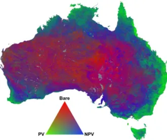
Figure3shows a national FCover product for Australia. The triangular ternary diagram can be read anti-clockwise between PV, nPV and BS. The interpretation of the colour coded fractions is based on the additive colour coding principle showing the relationship between the three endmembers. A quantitative Attribute Accuracy Assessment of the spectral unmixing approach and the overall error of the fractional ground cover RMSE is 11.8%, while the error margins vary for the three different layers where green vegetation has an RMSE of 11.0%, non-green vegetation 17.4%, and bare soil 12.5%. The validated Landsat derived fractional cover products are now used as key indicators for a range of environmental monitoring and management activities [22].
Figure 3. A multilayer FCover composite derived from Landsat 5 and available at the Terrestrial
2.3. Data Exploration for FCover Imagery
A FCover scene consists of three layers showing the fractions of each ground cover class in each layer. As part of our explanatory data analysis, we plotted histograms for all four years of the study period to review the distributions of PV, nPV and BS. Figure4shows the ground cover classes of the Landsat FCover bands combined in one histogram, along with the frequencies. We can clearly see that green vegetation has the least fractions but a high frequency, whereas non-green vegetation has higher fractions presented in one pixel.
(a) December 1987.
(b) December 1988.
(c) December 1989.
(d) December 1990.
Figure 4.Kernel Density plots of all Landsat FCover bands representing the individual fractions of
bare soil in red, green vegetation in green, not green vegetation in blue in one pixel. (a) December 1987,
(b) December 1988, (c) December 1989 and (d) December 1990.
The histograms indicated a roughly normal distribution for each of the classes. It can be seen that the green vegetation has the smallest fractions. In 1988, 1989 and 1990 the green vegetation was represented as the smallest fraction but with the highest frequency, except in 1987 where the bare soil
has the lowest percentages and the mode (represented as the highest bar) of the green vegetation shifts towards 20% and higher. This is an indicator that in 1987 the PV is more strongly represented than in the rest of the three years and therefore, we can infer that December 1987 was our wettest month. This is in accordance with the recorded rainfall data, described in the case study, where the monthly total is the highest in all of our FCover scenes. Moreover, the mode of green vegetation is smallest (around 12.5%) in 1990 and this reflects the lowest recorded monthly total and the lowest recorded daily rainfall in December 1990 as described earlier. Hence, 1990 is described as our driest year [34]. Figure5shows the four FCover scenes and their masked out areas.
(a) December 1987.
(b) December 1989.
(c) December 1988.
(d) December 1990.
Figure 5.FCover of Landsat Thematic Mapper (Landsat 5) scenes of four years showing white data gaps caused by masking out clouds and clouds shadows.
2.4. Data Pre-Processing and Spatial Aggregation
The aggregation involved several pre-processing steps. As one of the pre-processing steps, we created four evenly spaced spatial grid cell layers in four different spatial resolutions, showing the same geographic reference as the FCovers scenes and overlaid this on the raster image. The spatial grid layers were used as a vector overlay on the FCover scene showing varying coarseness of the grid cells extents ranging from the spatial resolution of 12,000 m, 6000 m, 3000 m and 1500 m. In addition, we ensured that the edges of the spatial grids lined up with the edges of the FCover pixels. Further,
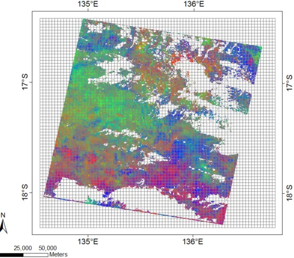
all missing values were removed and the arithmetic mean was calculated for each spatial grid cell. Figure6shows the spatial grid on top of the FCover scene at a resolution of 3,000 m. The figure also shows the extent of missing data, due to masking out obscuring elements such as cloud and cloud shadow.
Figure 6.Spatial grid cells at a resolution of 3000 m. The total number of cells 5530. The FCover data
are mapped to a even spaced grid where each grid cell contains 100×100 pixels and covers an area of
3000×3000 m. Please refer to Figure3for the triangular ternary diagram for the coloured relationships
of the three ground cover types.
The spatial resolution determines the geographic extent of each spatial grid cell in the FCover scene. One spatial grid cell in 12,000 m contained 400 × 400 FCover pixels each having a geographic resolution of 30×30 m and covering a total area of 12,000×12,000 m on the ground (400×30 m = 12,000 m). In contrast, the spatial grid resolution of 1500 m contains 50×50 pixels and covers an area of 1500×1500 m within the spatial grid cell. Table1lists all the spatial resolutions used in this study, the number of pixels contained within a spatial grid cell as an overlay on the FCover scene, the total area covered on the ground and the total number of spatial grid cells in the overlay used for the proposed aggregation scheme. The choice of the spatial resolutions allows for consistent arithmetic averages of FCover to be taken over the aggregated cells.
Table 1.Table of proposed data reduction scheme. The table shows the smallest resolution of 12,000 m up to the largest resolution of 1500 m and resulting total number of spatial grid cells used for the following spatial aggregation steps. By proposing our data reduction scheme we are not dealing with the original number of 54 million pixels per FCover scene organised in about 7000 rows and 8000 columns.
Spatial Resolution (m)
Number of Pixels in Grid Each Cell
Ground Covered by Each Grid Cell (m)
Total Number of Grid Cells
Coloured Outline of Spatial Grids
original 1×1 30×30 54 million FCover pixel
12,000 400×400 12,000×12,000 360 black
6000 200×200 6000×6000 1400 green
3000 100×100 3000×3000 5530 red
1500 50×50 1500×1500 21,980 grey
The four spatial grids demonstrated in Figure7were obtained using the open source software GME (Geospatial Modelling Environment). GME currently has dependencies on ArcGIS and R where it uses the statistical engine to drive some of the analysis tools.
Figure 7.Combination of all four spatial grids used as an overlay for the data delineation of green vegetation fractions out of FCover scenes. The thick black outline shows the resolution in 12,000 m, green in 6000 m, red in 3000 m and thin grey in 1500 m.
Each individual grid cell was used to calculate the arithmetic mean as a measure of central tendency of all the pixels contained within the spatial grid cell extent. As a result, one aggregated value of all green vegetation fractions contained within the grid cell extent represented each individual grid cell with the aggregated PV fraction. Since the spatial grid cells line up with the edges of the FCover pixels, adjacent and overlapping pixels will not be considered in the aggregation process.
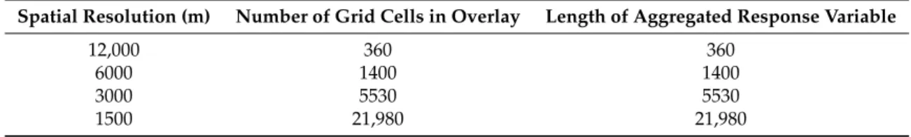
In addition to aggregating fractions of green vegetation spatial grid cells sizes we delineated the centroid coordinates as geographic latitude and longitude coordinates of each grid cell. The resultant csv file contained the response variable of aggregated fractions of green vegetation and the centroid coordinates in latitude (North-South direction) and in longitude (East-West direction). As discussed in the Introduction, no additional environmental data were used for the following modelling process using BRT. Altogether 16 csv files were created representing four spatial aggregations scheme for four years. Table2shows further details.
Table 2. The size of the pre-processed data set varies according to coarseness of the spatial aggregation resolutions.
Spatial Resolution (m) Number of Grid Cells in Overlay Length of Aggregated Response Variable
12,000 360 360
6000 1400 1400
3000 5530 5530
1500 21,980 21,980
2.5. Boosted Regression Trees
A boosted regression tree (BRT), also known as gradient boosted machine (GBM) or stochastic gradient boosting (SGB), is a non-parametric regression technique that combines a regression tree with a boosting algorithm [37] (AppendixA.1). This extension to the classical regression tree allows greater flexibility and predictive performance in modelling the data. The implementation of these methods used in this study can be found in the gbm R package [38].
A regression tree partitions multivariate data with a hierarchy of binary splits that define regions of the covariate space in which the response variable has similar values. These splits are defined by rules, distance metrics or information gain. The choice of variables and the value at which the split point occurs are determined in a recursive manner at each stage of the tree construction. The segmentation can be depicted as a tree-like structure, comprising nodes representing the selected factors, branches acting as if-else connectors between the nodes, and leaves representing terminal nodes containing the subsets of responses [39–41].
The performance of the simple base learner is improved by boosting, whereby a sequence of trees is grown, such that in each subsequent tree greater attention is paid to observations with greater prediction error. This is achieved by iteratively shifting the focus towards those observations until a stopping rule is reached. The shift is effected by up-weighting observations that were misclassified or had large residual errors in the previous iteration. The deeper tree accommodates more segments and hence captures more variance. This results in higher model complexity but also higher risk of overfitting the model to the data. The motivation behind boosting is that each tree can be quite shallow (a weak classifier) and thus fast to estimate, but by combining the predictive power of many weak classifiers, a classifier of arbitrary accuracy and precision can be created [42–44].
Next, the current approximationFm−1(x)is individually updated in all of the corresponding regions
Fm(x) =Fm−1(x) +ν·γlm1(x∈Rlm). (1)
The shrinkage parameter,ν, ranges from 0 to 1 and controls the learning rateγ, so each gradient
step is reduced by some factor between 0 and 1 of the learning rate. The value ofνis influenced by the
choice of loss functionψ.
Algorithm 1Stochastic Gradient Boosting algorithm. Training data{yi,xi1}iN Initialization F0(x) =arg minγ∑Ni=1ψ(yi,γ) form= 1 toMdo {π(i)}N 1 =randperm{i}1N Compute pseudo-residuals ˜ yπ(i)m=− " ∂ψ(yπ(i),F(xπ(i))) ∂F(xπ(i)) # F(x)=Fm−1(x) ,i=1, ˜N Fit a base learner to pseudo-residuals
{Rlm}L1 =L-terminal node tree
n ˜ yπ(i)m,xπ(i) oN˜ 1
Compute multiplierγlmby solving optimization problem γlm=arg min γ xπ(i
∑
)∈Rlm ψ yπ(i),Fm−1(xπ(i)) +γUpdate the model
Fm(x) =Fm−1(x) +ν·γlm1(x∈Rlm)
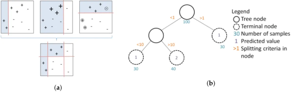
Figure8a shows four splits of the whole feature space of the data where the goal is to predict the plus symbols (+). The first three are binary splits that will be combined into one complex splitting rule (bottom). This yields a more accurate prediction result by separating the data allowing for flexible splitting boundaries. The first binary split (left) shown as the red vertical line has incorrectly predicted three observations indicated with a plus symbol. The misclassified observations get a higher weight to make sure those are favoured in the next splitting iteration (middle). The plot in the middle shows that three observations indicated with a minus symbol (−) are now misclassified. In the following step those misclassified observations will get higher weights again to be prioritised not to be included in the next splitting process. This time a horizontal line is generated. BRT is an ensemble approach and combines the first three binary splits above into one in order to create a complex prediction rule to split data allowing for identification of small areas of interests. This is the boosting part of BRT.
(a) (b)
Figure 8.(a) shows the combination of weak learners to one strong prediction rule used in the BRT
ensemble approach and (b) illustrated the hierarchical regression and binary splitting process along the
branches of the decision tree. (a) Binary splits indicated as red straight lines separate the data in grey
and white sections and create weak learners as seen in Equation (1). BRT as an ensemble approach
combines them to create complex prediction rules. Adapted from [46]. (b) Hierarchical regression and
binary splitting process showing observations in the nodes, predicted values in the terminal nodes and splitting criteria along the tree branches.
2.6. Implementation
The R package caret [47] was used for two tasks. The first was to split the data into training and test datasets (random partition that assigns 80% of the data in a training set and the remaining 20% to a test set) and the second task was to tune the hyperparameters for BRT modelling.
Typical hyperparameters include the
• shrinkage; (how quickly the algorithm adapts)
• tree complexity; the total number of trees in the final model (number of iterations)
• interaction depth; interaction between different nodes along the branch
• minimum observations in node; minimum number of training set samples in a node to commence splitting.
A feature of the BRT algorithm is that the performance can be tuned to accommodate specific data structures and characteristics through specification of hyperparameters. For our BRT model, the carat package was employed to find optimal values for the hyperparameters listed above. We used the automatic grid search method for searching optimal parameters, combined with other methods for estimating the performance of our gbm model based on our aggregated FCover data.
The outcome of the tuning process for all the 16 models was a recommendation of number of trees = 2500, interaction depth = 5, (only data of 1987 in 12,000 m recommended 3), shrinkage = 0.01, and minimum observations in node = 10. Those hyperparameters were then used to estimate the coefficients using the training data, and the prediction results are based on the test data set. Cross-Validation methods were used for the tuning process to help identify the hyperparameters and to restrict the number of iterations (hyperparameter tree complexity) to avoid overfitting when the local minimum has been reached. Empirically, it has been found that using a small value for shrinkage results in impressive improvements in a model’s generalisation ability [45]. The drawback of a lower learning rate is that more trees need to be generated, resulting in increased computational time. As described above, altogether 16 BRT models were created showing four years in four spatial resolutions; see Table1.
2.7. Quantitative Assessment of the Model Fit
The accuracy of the 16 BRT models was primarily analysed on the basis of the root mean square error (RMSE), the mean absolute error (MAE) and the median absolute error (MDAE), where we measured the difference between values predicted by a model and the values actually observed from the environment that is being modelled on the test dataset. In general, the RMSE is best when it is small, but there is no absolute good or bad threshold. The RMSE ranging between 3.3 and 1.1 indicates a good model fit throughout all resolutions.
3. Results
The computational environment was the R statistical modelling software version 3.3.3 [48] running inside Windows 7 SP1 (64-bit) on a 2.60 GHz Intel i7 CPU with 16 GB of RAM. All of the plots were generated in the R programming language [48] and maps throughout this paper were created using ArcGISR software by Esri. The GBM model implementations were taken from the gbm package [38]. We structure our results in three main groups. Since we want to investigate prediction accuracy using different spatial aggregations we first checked the residuals and how they spread around the mean of the regression line and the model fit in all the 16 models. Second, we evaluated the influence of each covariate on the response, shown by relative influence plots, or the functional relationships between the covariates and the prediction outcome indicated by partial dependency plots (AppendixA.2). Further, we investigated the relationship and distribution of the observed versus the predicted values in marginal plots. Last, we visualised the absolute error rate depending on the spatial resolution in all years and compared those with the elapsed time.
3.1. Comparison of Model Fit at Different Spatial Resolutions 3.1.1. Deviation of Residuals Around the Mean
Summary statistics and plots revealed that the residuals of the fitted models were relatively unbiased and homoscedastic. The residual plot of the worst model fit of the year 1988 in 1500 m and 12,000 m showed a slight tendency to heteroscedasticity due to a larger variance of the fitted values towards the maximum number of observations and further the resolution 12,000 m showed an unbalanced spread around the regression line towards under-predicted values shown in Figure9. These effects were not visible in any of the residual plots for the best model fit in the year 1990 demonstrated in Figure10.
Figure 9.Deviation of residuals around the mean of 1988 in all four resolutions as worst model fit.
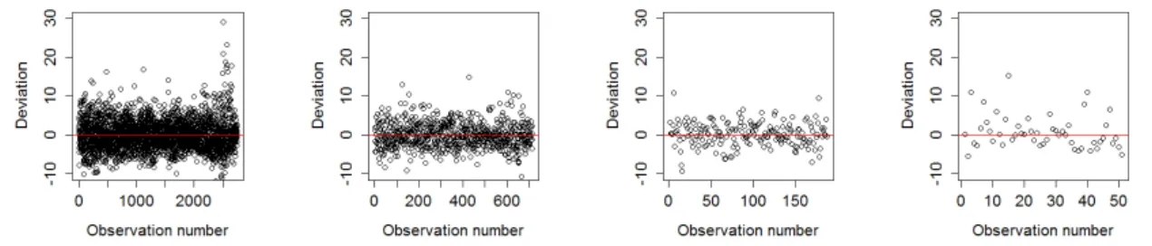
Figure 10.Deviation of residuals around the mean of 1990 in all four resolutions as best model fit.
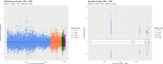
Figure11 shows the combined residuals over all years for all resolutions on the left and the corresponding box plots on the right.
The box plots show that the deviation of the residuals within the Inter Quartile Range (IQR), indicated as the white box around the zero line, is similar regardless of the spatial aggregation. However, there is more variation in the resolution of 1500 m than in any other resolutions. This can be explained by the argument that the loss functionψused in the BRT and the weighting of problematic
observations result in a similar deviation of the residuals at all aggregated spatial resolutions. We can see that the 6000 m resolution has the least error rates and is most symmetrically distributed around the black line showing the mean of the residuals. We conclude that aggregating from an initial geographic resolution of 30×30 m to 6000 m resolution resulting in the largest reduction in data volume without sacrificing precision of the prediction.
Figure 11.Deviation of residuals in all resolutions combined in one plot (left) and corresponding box
plots (right).
Table3shows the RMSE error rates for the four resolutions and four years. In general the smaller the RMSE error, the better the model fit.
Table 3.Comparison of the RMSE in all four years and resolutions.
Spatial Resolution (m) Year RMSE
12,000 1987 3.0583 1988 3.9691 1989 3.0056 1990 1.6151 6000 1987 2.8583 1988 3.1428 1989 3.1591 1990 1.9577 3000 1987 3.1120 1988 3.2134 1989 3.1543 1990 2.0731 1500 1987 3.4241 1988 3.8306 1989 3.4500 1990 2.3348
3.1.2. RMSE Comparisons between BRT and Linear Model (LM)
To evaluate the comparative performance of the BRT results, the data were also analysed using a linear regression model. The R package lm.br [49] was used to fit the model. We assume that green vegetation, denoted asYi, is linearly related to the covariates latitude and longitude, denoted asX1
andX2respectively, and the residualsεiare distributedN(0,σ2). The LM was formulated as follows: Yi=β0+β1∗X1i+β2∗X2i+εi.
The comparative goodness of fit of the LM and the BRT is shown in Table4. It is clear that under all four spatial resolutions, the BRT delivers a smaller RMSE. Based on this measure of performance, the BRT is argued to be an attractive alternative to the more common LM approach for analysing these types of data.
Table 4.Comparison of RMSE of LM and BRT on worst (1988) and best (1990) model fit.
Spatial Resolution (m) 1988 1990
Linear Model BRT Linear Model BRT
12,000 4.0551 3.9691 2.7933 1.6151
6000 4.9710 3.1428 3.0449 1.9577
3000 5.3688 3.2134 3.3028 2.0731
1500 5.5863 3.8306 3.5676 2.3348
3.1.3. Mean Absolute Error (MAE) and Median Absolute Error (MDAE)
In addition to the RMSE, we calculated the mean absolute error (MAE) and the median absolute error (MDAE) shown in Table5. MAE computes the average absolute difference between observed and predicted values as the vertical or horizontal distance between each point in a scatter plot. MDAE computes the median absolute difference between the two values. Please see Table5for details. In Section3.2.4, we see in the marginal plots that BRT under-predicts peak values. In Section3.3we use the absolute error to quantitatively assess the difference between observed and predicted values for all four spatial resolutions and all four years.
Table 5.MAE and MDAE of the worst (1988) and best model fit (1990) in four resolutions.
Spatial Resolution (m) Mean Absolute Error (Worst/Best) Median Absolute Error (Worst/Best)
12,000 2.752/1.236 2.236/0.836
6000 2.370/1.500 1.909/1.185
3000 2.489/1.613 2.053/1.305
1500 2.925/1.808 2.398/1.467
3.2. Variable Importance
3.2.1. Relative Influence of Covariates at Different Resolutions
One way of showing the relationships of the joint probability and contribution of our geographic coordinates in describing the response is through a relative influence plot. The relative influence is calculated by averaging the number of times a covariate is used in the tree building process, weighted by the squared improvement to the model as the result of each split. It is then scaled so the values sum to 100 [50]. Relative influence plots were used to compare the covariates with respect to their explanatory power. Regardless of the spatial resolution, among the two covariates used in the BRT model, the latitude (CenterY) is always more dominant than the longitude (CenterX). Moreover, the influence of the longitude (East/West direction) reduces as the spatial resolution is decreased towards 12,000 m. However, this is not a consistent reduction. In Figure12we demonstrate the influence of CenterX and CenterY covariates and their contribution towards predicting the aggregated green vegetation in the year 1989. The plots show the contribution at the best-estimated number of trees of 2500 iterations starting at 73.91% in 1500 m and reaching the maximal influence of 83.15% in 12,000 m. The relative influence of latitude (CenterY) dominates considerably over longitude (CenterX).
Figure 12.Relative influence plots of December 1989 in all four resolutions showing the contribution of the centroid coordinate of the latitude (CenterY) and longitude (CenterX).
3.2.2. Prediction Raster Maps
The Prediction Raster Maps clearly demonstrate a change in the marginal effect across spatial resolutions, seen as a smoothing effect towards the 12,000 m resolution; see Figure13.
3.2.3. Prediction Surface Plots
As fractional cover varies with the geographic coordinates, the partial dependence can be shown as a prediction surface plot. Here, the independent variables CenterX and CenterY are plotted against the model outcome ¯yafter considering the average effect of the other independent variable in the model. Since, we only have geographic coordinates as covariates we get a prediction surface plot showing the comparative influence of the latitude and the longitude as seen in Figure14.
3.2.4. Marginal Influence Plots
Marginal plots help in understanding the interaction effects of two variables by displaying the marginal relationship between the predicted aggregated fractions and the observed values of the test data set. Marginal plots also provide useful diagnostic information about the fitted model.
Figure15shows the marginal plots for the best model fit in the year 1990. The plots indicate that the BRT model under-predicts high observed values throughout all resolutions. This is especially apparent in the longer tails of the right-skewed histogram and density curves shown on the observed axis. In general, all plots exhibit a positive and relatively strong relationship, with a tendency towards clustering at the predicted values as seen by the vertical multi-modal histogram and density plot on the predicted axis. This is especially true in the resolution of 12,000 m where three clusters are evident, whereas in the resolution of 1500 m it seems there is more smoothing present. This is a feature of the BRT design, as described in Section2.5.
(a) December 1990 in the resolution of 12,000 m.
(b) December 1990 in the resolution of 6000 m.
(c) December 1990 in the resolution of 3000 m.
(d) December 1990 in the resolution of 1500 m.