FPGA Implementation of Sphere Detector for
Spatial Multiplexing MIMO System
Asma Mohamed, Abdel Halim Zekry, and Reem Ibrahim
Abstract—Multiple Input Multiple Output (MIMO (techniques use multiple antennas at both transmitter and receiver for increasing the channel reliability and enhancing the spectral efficiency of wireless communication system.MIMO Spatial Mul-tiplexing (SM) is a technology that can increase the channel capacity without additional spectral resources. The implemen-tation of MIMO detection techniques become a difficult mission as the computational complexity increases with the number of transmitting antenna and constellation size. So designing detec-tion techniques that can recover transmitted signals from Spatial Multiplexing (SM) MIMO with reduced complexity and high performance is challenging. In this survey, the general model of MIMO communication system is presented in addition to multiple MIMO Spatial Multiplexing (SM) detection techniques. These detection techniques are divided into different categories, such as linear detection, Non-linear detection and tree-search detection. Detailed discussions on the advantages and disadvantages of each detection algorithm are introduced. Hardware implementation of Sphere Decoder (SD) algorithm using VHDL/FPGA is also presented.
Keywords—Multiple Input Multiple Output (MIMO), Spatial Multiplexing(SM), Zero-Forcing (ZF), Minimum Mean Square Estimator (MMSE), Sorted QR Decomposition (SQRD), Sphere Decoder (SD).
I. INTRODUCTION
I
N the recent years, MIMO systems play an important role in increasing the channel capacity and improve the channel reliability. The main idea for the MIMO systems is the ability to turn multi-path propagation, which is an obstacle in the conventional wireless communication, into a benefit for users. MIMO techniques have been emerged as extensions to current wireless communication standards such as IEEE 802.11 which was organized with the aim of increasing the application throughput to at least 100Mbps by making modifications in the PHY and MAC layer. The demand for high speed transmission becomes challenging to the system designers. MIMO system uses several antennas at both transmitter and receiver to provide solution to increase data rates and reliability with acceptable bit error rate (BER).But the BER is dependent on the detection techniques that are used on the receiver side. The new wireless communication protocol like WiMAX, WI-Fi, LTE etc. is using MIMO technology to satisfy the increasing demand of high data rate [1].MIMO technology is classified into: MIMO spatial multiplexing technique and MIMO diversity technique [2]. MIMO diversity technique is A. Mohamed and A. zekry are with Electronics and Electrical Commu-nications Engineering Department, ASU University, Cairo, Egypt (e-mail: asmaa mohamed [email protected] , e-mail: [email protected]).R. Ibrahim is with Design Department managerVLSI Design Center Elec-tronics Factory, Cairo, Egypt (e-mail: [email protected]).
used to improve the reliability of transmission and Quality of Service (QoS) as it improves signal to noise ratio (SNR). Where the data stream is space time coded and then transmit-ted through different antennas which gives more reliability but the data rate is lower .In the diversity techniques, the same data stream is transmitted from multiple antennas or received at more than one antenna, so the receiver receives the same signal from different fading paths, and consequently the SNR is improved to provide high performance [3][4]. MIMO spatial multiplexing technique is used to increase the channel capacity linearly with the number of transmitting antennas, so high transmission rate is achieved without allocating more bandwidth or increasing the transmission power. In spatial multiplexing technique, independent data streams are simul-taneously transmitted through multiple transmit antennas and the received signal at each receive antenna corresponds to a combination of multiple data streams from all the transmit antennas [1].Recent researches have shown that usage of spatial multiplexing MIMO systems can increase the channel capacity without requiring extra-bandwidth or transmit power . In this research, we are interested in Spatial multiplexing MIMO and their detection techniques due to the strong need for such systems as the detection technique is an important part in the MIMO communication systems. The detection tech-niques are classified into Optimal detection technique such as Maximum likelihood (ML) [5,6] whose complexity increases exponentially with the size of constellation, and suboptimal ones. One of the suboptimal techniques is the Liner detection technique such as Zero forcing (ZF) and Minimum Mean square error (MMSE) [8] which is characterized by reduced complexity but they suffer from performance degradation. Nonlinear detection technique are also used such as Successive interference cancellation(SIC)[9,10,11] which is exposed to error propagation as well as Tree search detection technique such as sphere decoding algorithms [12,13]which can achieve quasi-ML performance as they can reach to ML solution with low computational complexity. In this paper, seeking the elec-tronic design of building blocks of communication systems, we will concentrate on Schnorr-Euchner sphere decoder algorithm where the algorithm is designed and implemented in field programmable gate arrays FPGA using VHDL. So, the paper is organized as follows: In Section II, the MIMO system model is provided. Next, the spatial multiplexing detection techniques are explained. The sphere detector is introduced in detailed in section III. FPGA hardware implementation of Schnorr-Euchner sphere decoder using VHDL is presented in Section IV. Finally, section V concludes the paper.
II. DETECTION TECHNIQUES
A. Mimo System Model
Fig. 1 shows a Spatial Multiplexing MIMO system consist-ing ofnT transmit antennas andnR receive antennas where the input stream of data is split into different independent sub streams. Assume that the transmitted vector is x = [x1 x2...xnT]T which is transmitted through sufficiently separated antennas. The transmitted signals reach the receiver via a rich-scattering environment [7]. So, the received vector becomes
y= Hx+n (1)
Where, y is the received (nR x 1) vector, H is (nR x nT) channel matrix . The transmitted vector elements are drawn independently from a constellation set Ω . The symbol n
is Gaussian noise vector (nR x1),whose elements are drawn from independent and identically distributed (i.i.d) circular symmetric Gaussian random variables.
Fig. 1. Spatial Multiplexing MIMO System.
B. MIMO detection techniquesl
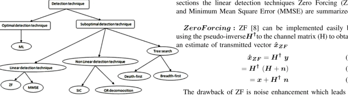
The main challenge resides in designing detection tech-niques that can recover the transmitted signals from Spatial Multiplexing (SM) MIMO with reduced complexity and high performance. MIMO detection techniques implementation is complex task, because the computation increases with the number of transmitting antennas and the symbol constellation size. Fig. 2 depicts the various detection techniques of the transmitted signals at the MIMO receiver. They are classified into optimal and suboptimal detection techniques.
Fig. 2. SM Detection techniques.
The optimal detection techniques are based on maximum likelihood algorithm where there are various suboptimal niques that can broadly classified into linear detection tech-niques such as zero forcing ZF and minimum mean square error MME, nonlinear detection techniques such as successive interference cancellation SIC and QR decomposition, as well as tree search such as depth-first and breadth first. For pointing out the main features of each detection algorithm, their basic operations will be outlined in the next sections.
1) Optimal Detection Technique: Maximum likelihood de-tection (MLD) is the optimum receiver for MIMO systems [5,6] ,but its implementation is very complex ,because the computational load increases exponentially depending on the number of transmitting antennas and modulation level.ML recovers the transmitted signal based on solving
∧ x = argmin x∈ΩnT k y − Hx k 2 (2) Wherexˆis the estimated vector,yis the received vector,His the channel matrix and x is the transmitted vector. The flow chart of the MLD algorithm is depicted in Fig. 3
Fig. 3. flowchart of Maximum likelihood algorithm
ML detection can’t be implemented directly, because the complexity increases exponentially when the size of constel-lation or the number of antennas increases. So, one goes to search for less complex detection algorithms.
2) Linear detection technique: The linear detection techniques are easy to implement as the received signal is filtered linearly, but it suffers from high degradation in error performance due to this linear filtering. In the next sections the linear detection techniques Zero Forcing (ZF) and Minimum Mean Square Error (MMSE) are summarized.
ZeroF orcing : ZF [8] can be implemented easily by using the pseudo-inverseH†to the channel matrix (H) to obtain an estimate of transmitted vectorxˆZF
ˆ
xZF =H† y (3)
=H† (H+n) (4)
=x+H† n (5)
The drawback of ZF is noise enhancement which leads to high performance degradation.
M inimum M ean Square Error: MMSE [8] can overcome the problem of noise enhancement in ZF by using filtering matrix.
(HHH+ σ2n I)−1HH
The estimate of transmitted vectorxM M SE is
xM M SE = (HHH+ σ2n I)
−1
HH y (6)
3) Nonlinear detection techniques : They are more complex than linear techniques and have improved performance than linear techniques, as they use decision feedback detection algorithm .Nonlinear detection techniques are Successive Interference Cancellation (SIC)(such as V-BLAST) and QR decomposition.
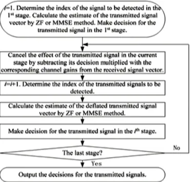
Successive Interf erence Cancellation(SIC) : SIC uses decision feedback detection to detect symbols successively, where it detects the most reliable symbol of the transmitted vector and use it to improve the detection of other symbols such as (V-BLAST)[9].V-BLAST detects the most reliable symbol of the transmitted vector using ZF or MMSE filtering matrix and then subtract the interference from the detected symbol to generate modified received vector .This process is repeated in iterative way until all the symbols of the transmitted vector are detected. V-BLAST suffers from error propagation problem, but to reduce the effect of error propagation one uses sorted ZF-VBLAST (SZF-VBLAST) or sorted MMSE-VBLAST (SMMSE-VBLAST). The flow chart of the SIC algorithm is depicted in Fig. 4 to show the major processing steps in the algorithm. The main drawback of SIC (V-BLAST) is its computational complexity, as the pseudo inverse for the channel matrix is calculated at each detection step. QR decomposition: QR decomposition
Fig. 4. flowchart of SIC algorithm
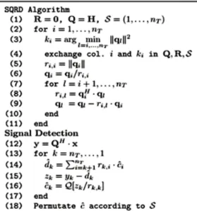
[10] reduces the computational bottleneck in V-BLAST, where the MIMO channel matrix (H) is factorized into unitary (nR xnT) matrix (Q) which has orthogonal columns of unit norm and upper triangular (nT x nT) matrix (R) by using Gram-Schmidt process.
H=Q.R (6)
The received vectory becomes
y=H.x+n =Q.Rx+n (7)
QHy=QHQRx+QHn (8)
ˇ
y=R.x+v (9)
Where, yˇ is the modified received vector(QHy), v is the modified noise vector (QHn).
The transmitted symbolsxcan be detected from the modi-fied received vectoryˇby using a Gauss elimination algorithm. The (kth) element (yˇk) of the modified received vector ( yˇ) is given by ˇ yk=rkk∗xˆkk+ nR X i=k+1 rki.ˆxi+ vk (10)
All the transmitted symbols can be detected by starting from the last element of the received vector (ˇynR) and using
successive interference cancellation (SIC) scheme.
ˆ xk=Q yˇ k− P nR i=k+1rki.xi rkk (11) So the computational complexity decreases. Fig. 5 shows the list of the signal processing used in the QR decomposition al-gorithm. The drawback of this technique is error propagation. To reduce this error propagation one uses sorted QR decom-position [11]. This can be done by permuting the columns of the channel matrix (H) prior to the decomposition, where the transmitted signal over the highest reliability channel should be detected first, then SIC is performed and the second highest reliability channel is detected second, and SIC is performed and so on until all the transmitted signals are detected. So, the first detected signal is that transmitted with highest SNR and the last detected signal is that transmitted with smallest SNR.
4) Tree search detection technique : It is used to achieve quasi-ML performance, where it can reach to ML accuracy with low computational complexity. The idea behind this technique is to reduce the number of possible combinations of constellation points tested by the ML metric using a radius in the lattice, where the MLD search problem is presented as a tree whose nodes act as the symbol’s candidates. The most popular tree search detection technique is Sphere decoding. It will be studied, designed and FPGA implemented in the next section.
Fig. 5. SQRD algorithm and signal detection
III. SPHERE DECODER
Sphere Decoding (SD) was originally introduced in 1985 by Finke and Pohst [12] as a technique for solving the Closest Lattice Point Problem (CLPP).The SD was first used in communications in 1993 for soft decoding of the Golay code by Viterbi and Bigleri [13].Currently, it has been used as the most powerful and promising mean of finding the Maximum Likelihood (ML) solution for the detection problem of Multiple-Input Multiple-Output (MIMO) communication systems. The principle of SD is to search for the closet constellation point to the received signal within a hyper sphere of radius (d) centered at the tip of the received vector (y).The Geometric representation of the SD algorithm is shown in Fig.6 As mentioned in the introduction the ML detection
Fig. 6. Geometric representation of the SD algorithm
has exponential computational complexity, due to the massive search through the whole lattice.The SD restrict the searching over certain subset that contain the ML solution [14][15].Con-sider the channel matrix (H) is factorized into unitary matrix (Q) and upper triangular matrix (R) so the system model can be written as ˇ y=R.x+v (12) Where ˇ y=QHy (13) v=QHn (14)
So the ML detection problem can be written as
ˆ
x=arg minkyˇ − Rx k 2 (15) The SD solves the equation by searching the vectors that belong to certain subset that satisfying the sphere constraint (SC). kyˇ − Rx k 2≤d2 (16) So, ˆ xSD=argxmin∈ΩnT(kyˇ − Rx k 2 ≤d2) (17) To search the tree and calculate partial Euclidean distances, first build the Tree that contains all the candidate lattice points; the Tree must have number of levels equal to the number of the transmit antennas, and each symbol value is represented by node in the Tree. To solve (17) one begins search from the top level (root) (at level (nT + 1) ) of the Tree. And every time the search transfer from a node in level (i) ( parent node) to the nodes that connected to it in level (i−1) (children nodes).Evaluate the partial Euclidean distances (PED) of the children nodes, where PED is the distance between two successive levels ( (i−1) and (i) in the tree, it can be called the branch weight. PED can be expressed by: P ED=ei x(i) = ˇyi− nT X j=i Rij xj (18)
Then evaluate the accumulated PEDTi x(i )of each branch as: Ti x(i ) = Ti+1 x(i+1 )+ |ei x(i)| 2 (19) We start at level i = nT and set TnT+1 x
(nT+1 ) = 0
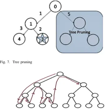
When the accumulated PED of a parent node is greater than (d), its children nodes can be pruned in advance, this lead to less visited points and hence faster tree-search.
When the accumulated PED of a child node is smaller than (d), then (d) is updated and the radius of the sphere becomes the smaller accumulated PED.
The child node with the lowest accumulated PED (T1 x(1 )
) corresponds to the ML solution.Fig.7 shows the process of tree pruning.
Tree search is based on different strategies where some of them can be found in [16], [17], [18], [19].These strategies are classified into two main types; depth-first and breadth-first. In Depth-First algorithms [20], [21], [22]the tree is explored starting from the root descending to the leaf nodes, but each child node is explored from left to right.Fig.8 shows a Depth-First strategy.
In the Breadth-First algorithms the tree is explored descending to the leaf nodes, but exploring level by level. Fig.9 shows a
Fig. 7. Tree pruning
Fig. 8. decoding tree with a Depth-First strategy
Breadth-First strategy .This means that exploring every child node in the same level before starting to explore the following level.
Fig. 9. Decoding tree with a Breadth-First strategy
Fincke-Pohst Strategy (FP)is one of the depth-first SD algo-rithms. In this strategy the search radius must be initialized before starting the search.Fig.10 shows FP sphere decoding algorithm, where the blue circle indicates the node in the radius and red circle indicates node out the radius. Tree search starts from the tree root down to leaf node and from left to right. When the PED of a node exceeds the search radius, this node and its children nodes are discarded from the tree. After completed search, there are different possible solutions in the tree inside the sphere. The ML estimate would be the solution with the least PED among these final candidates.
The critical issue of this strategy is the sphere search radius, where if the sphere radius is too small, there can be no can-didate solutions detected and the algorithm will not perform correctly. On the other hand, if the sphere radius is too large, there are too many candidate solutions may be detected and the complexity of the algorithm can be equal the complexity of the ML detector without any advantage over existing methods.
Fig. 10. Fincke and Phost Sphere Decoding Algorithm
There are several ways to estimate the sphere radius [23], where a recommended choice for the sphere radius is obtained by calculating the distance between the received vector and the solution provided by suboptimal detection Technique such as ZF or MMSE.
d=kyˇ − RxˆZF k
2
(20) Other authors suggest that choosing the sphere radius as scaled version of the noise variance, because it is logical to consider that the transmitted vector will be deviated from its original position a distance related to the noise variance that present in the system.
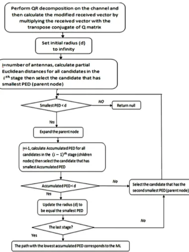
Schnorr-Euchner strategy (SE) also performs the depth-first SD algorithm. It adds a significant refinement to the FP strategy; the SE-SD calculates the PEDs of all the children nodes from a certain node and then explores them according to the increasing order of their PEDs. This modification allows reaching to the leaf node faster than (FP), but the number of computed PEDs remains the same as in the (FP). So, (SE) proposed another modification to solve this problem, the sphere radius is reduced when a leaf node is found and so on. Therefore, in SE algorithm the search radius can be initialized to infinity and be updated every time a new leaf node is discovered. So the issue of selecting the initial sphere radius becomes not critical. Schnorr-Euchner sphere decoding algorithm is depicted in fig.11, where the blue circle indicates the node in the radius and red circle indicates node out the radius.
Fig. 11. Schnorr-Euchner Sphere Decoding Algorithm
IV. HARDWARE IMPLEMENTATION OF SCHNORR-EUCHNER SPHERE DECODER: In this section we describe the VHDL implementation of 2X2 MIMO system with QPSK modulation and Schnorr-Euchner Sphere decoder algorithm. Modelsim simulator is used in order to perform simulation of the VHDL code of this algorithm. The code is developed according to signal processing flow chart depicted in Fig.12, where the input data is obtained by generating 0s,1s with equal probability. Then
we make QPSK mapping to generate the first symbol which is transmitted by the first antenna and the second symbol which is transmitted by the second antenna according to table.1. Then the symbols are transmitted through MIMO channel with additive white Gaussian noise AWGN.
Fig. 12. flowchart indicates the signal processing steps
The MIMO receiver is composed of Schnorr- Euchner Sphere decoding detector an addition to a demapper. The SE sphere decoding algorithm is performed by making QR decomposition for the MIMO channel matrix and setting the initial radius to infinity, then calculating the PED of each node in the tree starting from the root of the tree as explained in Fig.11. When reaching to ML solution, it goes through demapper to get the transmitted bits again. The flowchart in Fig.13 indicates the SE Sphere decoding algorithm.
We find that the PED that calculated in the SE sphere decoding algorithm is always floating number. So, we want to present the precision of the floating point because for example we must distinguish between PEDs of (4.9) and (5.1) to choose the correct branch. To represent the floating point in FPGA we must use the standard technique of floating point representation. The standard techniques of floating point representation are 32-bit floating point representation and 64-bit floating point representation. We used 32-bit floating point representation of the symbols to provide high accuracy of calculations in Schnorr-Euchner Sphere decoder. So a special adder, special multiplier and special sorting function are built to deal with the floating point numbers.
A 32-bit floating point adder block diagram is shown in Fig.14 where it has four inputs, two of them are the floating point numbers (32-bit) that to be added or subtracted, the third is the clock, while the input Add/Sub is control which
Fig. 13. flowchart of Schnorr- Euchner Sphere decoding algorithm
selects addition or subtraction process. It has also one output pin which indicates the result of addition/subtraction.
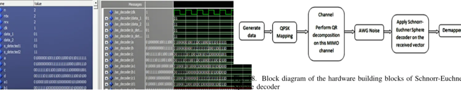
Fig. 14. Block diagram of the special adder for 32-bit floating point The designed adder simulation result is shown in Fig.15. Where the first input (a) is (01000011101010000011001110100000) which equivalent to (336.4) and the second input (b) is (00111101110011001100001110010111) which equivalent to (0.1) the result is (z) (01000011101010000100000001101100) which equivalent to (336.5).
A 32-bit floating point multiplier block diagram is shown in Fig.16.It consists of two input pins which are the floating point numbers (32-bit) that should be multiplied, and one output pin which indicates the result of multiplication. The multiplier simulation result is shown in Fig.17. Where the first input (x) is (11000000010000000000000000000000) which equivalent to (-3) and the other input (y) is (01000000010010100110001100100000) which
Fig. 19. ModelSim wave diagram of Schnorr-Euchner Sphere decoder
Fig. 20. Xilinx area report of Schnorr-Euchner Sphere decoder
Fig. 15. ModelSim wave diagram for the 32-bit floating point adder/subtraction output
Fig. 16. Block diagram of the special multiplier for 32-bit floating point
equivalent to (3.16), the multiplication result (z) is (11000001000101111100101001011000) which equivalent to (-9.48)
Fig. 17. ModelSim wave diagram for the 32-bit floating point multiplier output
The methodology used for simulation and implementation SE sphere decoder is shown in Fig.18 where it contains the following digital functions:
a) Generate data. b) QPSK Mapping.
c) Transmit the encoded data through two different antennas. d) Perform QR decomposition on the MIMO channel which under AWGN.
e) Apply Schnorr-Euchner Sphere decoder on the received vector.
f) Demapping process to get the transmitted bits again.
Fig. 18. Block diagram of the hardware building blocks of Schnorr-Euchner Sphere decoder
The wave diagram simulation of SE sphere decoder on Mod-elsim simulator is shown in Fig.19, where data 1 (01) is the transmitted data from the first antenna, data 2 (11) is the transmitted data from the second antenna and s detected1 (01) is the detected data from the first antenna, s detected2 (11) is the detected data from the second antenna.
The synthesis report of our designed Schnorr-Euchner Sphere decoder in the Xilinx Virtex 6 FPGA using the part number xc6vlx760-1ff1760 is summarized in the area report shown in Fig.20.
In this technique we use a lot of slices LUTs and this is an expected result, as we use floating point technique and iterative algorithm. Also the number of LUTs increase due to the augmentation in the number of adders/subtractors and multipliers required for the algorithm that are implemented on the FPGA.
V. CONCOLUSION
MIMO communication systems have used spatial multiplexing technique to increase the channel capacity and enhance the spectral efficiency. The main challenge of MIMO SM is the detection techniques. In this paper several detection techniques for MIMO SM such as linear,nonlinear and tree search are introduced and analyzed to illustrate the advantages and disadvantages of each detection technique. In general, linear detection techniques such as ZF and MMSE have less complexity, but suffer from poor performance. Nonlinear techniques such as VBLAST are introduced, but their performance is limited due to error propagation and the computational Complexity. Decomposition based algorithms can be used to reduce the computational complexity, but suffer from error propagation. The tree search algorithm such as SD achieves quasi-ML performance, as it reaches to ML solution with low computational complexity. Schnorr-Euchner Sphere decoder algorithm is designed and implemented on FPGA using VHDL. The main issue of the design is using 32 bit floating point arithmetic to achieve the required high precision. References:
[1] JeffreyG.Andrews, ArunabhaGhosh, and Rais Mohamed, “Fundamentals of WiMAX: Understanding Broadband Wire-less Networking”, Prentice Hall, 2007
[2] JanMietzner, RobertSchober, Lutz Lampe, Wolfgang H. Gerstacker, Peter A. Hoeher, “Multiple-Antenna Techniques for Wireless Communications – A Comprehensive iterature Survey,” IEEE communications survey and tutorials, Vol II No 2, Second quarter 2009.
[3] G. J. Foschini, “Layered space-time architecture for wire-less communication in a fading environment when using mul-tielement antennas,” Bell Syst. Tech. J., pp. 41–59, Autumn 1996.
[4] G. J. Foschini and M. J. Gans, “On limits of wireless communications in a fading environment when using multiple antennas,” Kluwer Wireless Pers. Commun., vol. 6, pp. 311– 335, Mar. 1998
[5] W. Van Etten, “Maximum likelihood receiver for multiple channel transmission systems,” IEEE Trans. on Communica-tions, pp. 276-283, Feb. 1976.
[6] Z. Xu and R. D. Murch, “Performance analysis of maxi-mum likelihood detectionin a MIMO antenna system,” IEEE Trans. Commun., vol. 50, no. 2, pp. 187– 191, Feb. 2002 [7] P. Wolniansky, G. Foschini, G. Golden, and R. Valenzuela, “V-BLAST: An architecture for realizing very high data rates over the rich-scattering wireless channel,” in Proc. URSI In-ternational Symposium on Signals, Systems, and Electronics, pp. 295-300, Oct.
[8] J. Paulraj, D. A. Gore, R. U. Nabar, and H. Boelcskei, “Anoverview of MIMO communications – A key to gigabit wireless,” Proc. IEEE, vol. 92, no. 2, pp. 198–218, Feb. 2004. [9] P. W. Wolniansky, G. J. Foschini, G. D. Golden, and R. A. Valenzuela, “VBLAST: An architecture for realizing very high data rates over the rich-scattering wireless channel,” URSI Int. Symp. on Signals, Systems and Electronics, (Pisa, Italy), pp. 295300, Sep. 1998
[10] D. Shiu and J.M. Kahn,\Layered Space-Time Codes for Wireless Communications using Multiple TransmitAntennas,” in IEEE Proceedings of International Conference on Commu-nications (ICC’99), Vancouver, B.C.,June 6-10 1999
[11] D. W¨ubben, J. Rinas, R. B¨ohnke, V. K¨uhn, and K.D. Kammeyer, “Efficient Algorithm for Detecting Layered Space-Time Codes”,4thInt. ITG Conference on Source and Channel
Coding, Berlin, January 2002
[12] U. Finke, and M. Pohst, “Improved methods for calculat-ing vectors of short length in a lattice, includcalculat-ing a complexity
analysis,” Mathematics of Computation, vol.44, no. 170, pp. 463-471, April 1985.
[13] E. Viterbo and E. Bigleri, “A universal lattice decoder,” In 14eme Colloque GRETSI, pp. 611-614, September 1993. [14] E. Viterbo and J. Boutros, “A universal lattice code decoder for fading channels,” IEEE Trans. Inform. Theory, vol. 45, no. 5, pp. 1639–1642, July 1999.
[15] M. O. Damen, H. E. Gamal, and G. Caire, “On maximum likelihood detection and the search for the closest lattice point,” IEEE Trans. Inform. Theory, vol. 49, no.10, pp. 2389– 2402, Oct. 2003.
[16] B. Hassibi and H. Vikalo, “On Sphere Decoding algo-rithm. Part I,the expected complexity,”IEEE Transactions on Signal Processing,vol. 54, no. 5, pp. 2806–2818, August 2005. [17] Z. Guo and P. Nilsson, “Algorithm and implementation of the K-BestSphereDecoding for MIMO Detection,”IEEE Journal on SelectedAreas in Communications, vol. 24, no. 3, pp. 491–503, March 2006.
[18] M. O. Damen, H. E. Gamal, and G. Caire, “On Maximum-Likelihood detection and the search for the closest lattice point,”IEEE Transactions on Information Theory, vol. 49, no. 10, pp. 2389–2402, October2003.
[19] K. Su, “Efficient Maximum Likelihood detection for com-municationover MIMO channels,” University of Cambridge, Technical Report,February 2005.
[20] C. P. Schnorr and M. Euchner, “Lattice basis reduction: Improved practical algorithms and solving subset sum prob-lems,” Math. Program., vol. 66,pp. 181–191,1994.
[21] E. Agrell, T. Eriksson, A. Vardy, and K. Zegar, “Closet point search in lattices,”IEEE Trans. Inf. Theory, vol. 48, pp. 2201–2214, Aug. 2002.
[22] A. D. Murugan, H. E. Gamal, M. O. Damen, and G. Caire, “A unified frameworkfortree search decoding: rediscovering the sequential decoder,” IEEE Trans. Inf.Theory, vol. 52, no. 3, pp. 933–953, Mar. 2006
[23] B. Hassibi and H. Vikalo, “On Sphere Decoding algo-rithm. Part I,the expected complexity,”IEEE Transactions on Signal Processing,vol. 54, no. 5, pp. 2806–2818, August 2005.