remote sensing
ArticleA Novel Approach for Estimation of Above-Ground
Biomass of Sugar Beet Based on Wavelength Selection
and Optimized Support Vector Machine
Jing Zhang1,2, Haiqing Tian1,*, Di Wang1, Haijun Li1and Abdul Mounem Mouazen2
1 College of Mechanical and Electrical Engineering, Inner Mongolia Agricultural University, Hohhot 010018, China; [email protected] (J.Z.); [email protected] (D.W.); [email protected] (H.L.) 2 Department of Environment, Ghent University, Coupure Links 653, 9000 Gent, Belgium;
* Correspondence: [email protected]; Tel.:+86-1594-701-9846
Received: 9 January 2020; Accepted: 10 February 2020; Published: 13 February 2020 Abstract:Timely diagnosis of sugar beet above-ground biomass (AGB) is critical for the prediction of yield and optimal precision crop management. This study established an optimal quantitative prediction model of AGB of sugar beet by using hyperspectral data. Three experiment campaigns in 2014, 2015 and 2018 were conducted to collect ground-based hyperspectral data at three different growth stages, across different sites, for different cultivars and nitrogen (N) application rates. A competitive adaptive reweighted sampling (CARS) algorithm was applied to select the most sensitive wavelengths to AGB. This was followed by developing a novel modified differential evolution grey wolf optimization algorithm (MDE–GWO) by introducing differential evolution algorithm (DE) and dynamic non-linear convergence factor to grey wolf optimization algorithm (GWO) to optimize the parameters c and γ of a support vector machine (SVM) model for the prediction of AGB. The prediction performance of SVM models under the three GWO, DE–GWO and MDE–GWO optimization methods for CARS selected wavelengths and whole spectral data was examined. Results showed that CARS resulted in a huge wavelength reduction of 97.4% for the rapid growth stage of leaf cluster, 97.2% for the sugar growth stage and 97.4% for the sugar accumulation stage. Models resulted after CARS wavelength selection were found to be more accurate than models developed using the entire spectral data. The best prediction accuracy was achieved after the MDE–GWO optimization of SVM model parameters for the prediction of AGB in sugar beet, independent of growing stage, years, sites and cultivars. The best coefficient of determination (R2), root mean square error (RMSE) and residual prediction deviation (RPD) ranged, respectively, from 0.74 to 0.80, 46.17 to 65.68 g/m2and 1.42 to 1.97 for the rapid growth stage of leaf cluster, 0.78 to 0.80, 30.16 to 37.03 g/m2and 1.69 to 2.03 for the sugar growth stage, and 0.69 to 0.74, 40.17 to 104.08 g/m2 and 1.61 to 1.95 for the sugar accumulation stage. It can be concluded that the methodology proposed can be implemented for the prediction of AGB of sugar beet using proximal hyperspectral sensors under a wide range of environmental conditions.
Keywords: sugar beet; above-ground biomass; grey wolf optimization; support vector machine; hyperspectral sensing
1. Introduction
Sugar beet is one of the most important crops for sugar production that is stored in roots. As the development of roots (below ground) and leaves (above-ground) biomass is closely correlated to each other, above-ground biomass (AGB) is considered as an essential parameter for plant growth status, yield and harvest quality [1,2]. Therefore, accurate estimation of AGB is essential for sugar
Remote Sens.2020,12, 620 2 of 22
beet monitoring and yield prediction. Other applications of information about AGB are site-specific fertilization and pesticide applications. Measurement of AGB can be done either by traditional methods, the use of proximal crop sensing or remote sensing techniques. However, the traditional method based on human evaluation is far more demanding in terms of timeliness, spatial resolution and practicability, compared to the proximal and remote sensing methods [3,4]. With recent advancements in spectral analysis over the past few decades, proximal and remote sensing techniques have attracted abundant attention for crop monitoring and yield prediction, due to their fast, cost-effective and non-destructive nature [5].
Hyperspectral images (HSI) contain hundreds of narrow continuous spectral wavelengths, each indicating a one-dimensional feature. Both spectral and spatial information are captured simultaneously with hyperspectral cameras [6]. Due to the high spectral resolution, HSI has the potentiality to predict physical objects, while also yielding massive data. The hyperspectral data is not only highly correlated, but also contains useless information and noise, which affects the detection accuracy of the target parameters. Therefore, it can be hypothesized that feature selection is one of the most important spectra pre-processing approaches to exclude redundant information and improve the prediction accuracy of a target parameter [7,8]. Competitive adaptive reweighted sampling (CARS), a variable selection approach, has been developed and successfully implemented for the selection of sensitive bands to specific plant variables under consideration, such as canopy nitrogen content and soluble solid contents [9,10]. Once band selection is optimized, quantitative modeling using linear or nonlinear techniques is followed to build calibration models to predict target variables.
Since the relationship between the spectral data and the target variable is nonlinear in the majority of case studies, a support vector machine (SVM) algorithm that can deal with both linear and nonlinear problems, with high dimensionality and local minima, was widely used in the field of spectral analysis. SVM has been successfully applied to model hyperspectral data for the prediction of plant biomass, leave area index (LAI) and nitrogen and chlorophyll concentration [11–14]. Although results confirmed that SVM is one of the most efficient methods in creating reliable quantitative models for the named crop properties, it is not always the case, as stated by Tarabalka et al. [15]. The accuracy, stability and generalization of SVM are determined by some parameters, such as penalty factor (c) and kernel parameter (γ), which change with data [16]. Parameter optimization is critical for improving the prediction performance of SVM models. Grey wolf optimization algorithm (GWO) is a newly proposed optimization algorithm. Currently, GWO has been applied in many fields, such as engineering [17], feature selection, image processing [18] and machine learning [19]. However, the accuracy of the traditional GWO is reported to be disappointingly low [20]. Due to the poor diversity of the population and the linearly decreasing control parameter, GWO is prone to premature convergence with low convergence accuracy when dealing with multimodal problems. Several optimization methods to solve those deficiencies of GWO have been proposed. Integrating the differential evolution (DE) algorithm into the grey wolf optimization algorithm (DE–GWO) to preserve the diversity of the population can avoid the local minimum and slow convergence problems associated with GWO [21]. However, the DE–GWO algorithm still faces a critical problem of how to keep the balance between the exploration ability and exploitation ability [22], referring to the global search ability and local search ability of GWO, respectively. Although the DE algorithm improves the global research ability of GWO, the relationship of exploration ability and exploitation ability in the DE–GWO algorithm is unbalanced, which is the main reason for the low accuracy. Therefore, the balance between the above mentioned two abilities is crucial for the DE–GWO. To overcome this problem, researchers [23,24] found that improving the convergence factor of GWO, by changing the original linear convergence factor to nonlinear convergence factors, such as sinusoidal curve, logarithmic curve and conic curve, is a suitable approach. However, in practice, due to the complexity of various datasets, the nonlinear convergence factors did not overcome all optimization problems to guarantee ideal prediction results. Therefore, in order to improve the predictive performance of SVM models for the assessment of AGB in sugar beet using HSI data, a modified DE–GWO algorithm (MDE–GWO) is needed, based on an
Remote Sens.2020,12, 620 3 of 22
improved algorithm of convergence factor to optimize the parameters of SVM that is hoped to result in more accurate prediction results.
This paper is the first to evaluate the feasibility of a novel MDE–GWO algorithm for improving the prediction accuracy of SVM models of AGB in sugar beet. The objectives of this study are (1) to determine the most important wavelengths for the assessment of AGB in sugar beet, (2) to develop a nonlinear convergence factor for DE–GWO to improve the prediction accuracy of SVM model and (3) to demonstrate the feasibility of MDE–GWO for the optimization of SVM models.
2. Materials and Methods
2.1. Experimental Design and Crop Growing
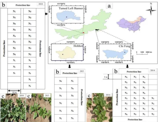
Three experiments were conducted in 2014, 2015 and 2018 at different locations in Inner Mongolia Autonomous Region, China, which were laid out in a randomized complete block split-plot design with one factor (N level), as shown in Figure1. In the year 2014, the study area was located in Tai Pingdi town (119◦240E, 42◦290N) of Song Shan District, Chi Feng city, and included seven levels of N (0, 15, 32, 76, 108, 163 and 217 kg/hm2) with four replicates. In the year 2015, the study area was located in an experimental farm (111◦410E, 40◦480N) of the Inner Mongolia Agricultural University, in Hohhot city, and included four levels of N (0, 80, 120 and 200 kg/hm2) with three replicates. In the year 2018, the study area was located in Ma Heli village (111◦130E, 40◦380N) of Tumd Left Banner, in Hohhot city, and included six levels of N (0, 70, 90, 116, 130 and 150 kg/hm2) with four replicates. The N treatments were randomly assigned into plots (Figure1), each having approximately 50 m2(5 m by 10 m) area. Sugar beet was transplanted with 25 cm by 50 cm spacing. All plots were fertilized with 1.2 kg/plot potassium chloride and 3.8 kg/plot calcium superphosphate. The entire amount of phosphorus, potassium and nitrogen fertilizer was applied prior to seeding as basal fertilizer. Other detailed management information is shown in Table1. For disease and pest control, pesticides were applied following the local standard practices. Sugar beet was grown once a year and the cropping season started from May (transplanting) and ended up in October (harvesting).
Remote Sens. 2020, 12, x FOR PEER REVIEW 3 of 23
improved algorithm of convergence factor to optimize the parameters of SVM that is hoped to result in more accurate prediction results.
This paper is the first to evaluate the feasibility of a novel MDE–GWO algorithm for improving the prediction accuracy of SVM models of AGB in sugar beet. The objectives of this study are (1) to determine the most important wavelengths for the assessment of AGB in sugar beet, (2) to develop a nonlinear convergence factor for DE–GWO to improve the prediction accuracy of SVM model and (3) to demonstrate the feasibility of MDE–GWO for the optimization of SVM models.
2. Materials and Methods
2.1. Experimental Design and Crop Growing
Three experiments were conducted in 2014, 2015 and 2018 at different locations in Inner Mongolia Autonomous Region, China, which were laid out in a randomized complete block split-plot design with one factor (N level), as shown in Figure 1. In the year 2014, the study area was located in Tai Pingdi town (119°24′E, 42°29′N) of Song Shan District, Chi Feng city, and included seven levels of N (0, 15, 32.5, 76, 108.5, 163 and 217.5 kg/hm2) with four replicates. In the year 2015, the study area
was located in an experimental farm (111°41′E, 40°48′N) of the Inner Mongolia Agricultural University, in Hohhot city, and included four levels of N (0, 80, 120 and 200 kg/hm2) with three
replicates. In the year 2018, the study area was located in Ma Heli village (111°13′E, 40°38′N) of Tumd Left Banner, in Hohhot city, and included six levels of N (0, 70, 90, 116, 130 and 150 kg/hm2) with four
replicates. The N treatments were randomly assigned into plots (Figure 1), each having approximately 50 m2 (5 m by 10 m) area. Sugar beet was transplanted with 25 cm by 50 cm spacing.
All plots were fertilized with 1.2 kg/plot potassium chloride and 3.8 kg/plot calcium superphosphate. The entire amount of phosphorus, potassium and nitrogen fertilizer was applied prior to seeding as basal fertilizer. Other detailed management information is shown in Table 1. For disease and pest control, pesticides were applied following the local standard practices. Sugar beet was grown once a year and the cropping season started from May (transplanting) and ended up in October (harvesting).
Figure 1. Location of the study sites (a), experimental layout showing plots (5 m by 10 m), different levels of nitrogen fertilizer (e.g., N0, N1, N2, N3, N4, N5 and N6) applied (b) and photographs of sugar beet plants in 2014, 2015 and 2018 experiments (c).
Figure 1.Location of the study sites (a), experimental layout showing plots (5 m by 10 m), different levels of nitrogen fertilizer (e.g., N0, N1, N2, N3, N4, N5and N6) applied (b) and photographs of sugar beet plants in 2014, 2015 and 2018 experiments (c).
Remote Sens.2020,12, 620 4 of 22
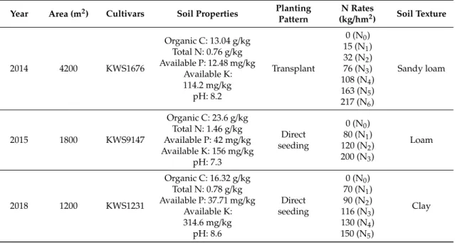
Table 1.Management information of the sugar beet experiment in the three experimental sites.
Year Area (m2) Cultivars Soil Properties Planting
Pattern N Rates (kg/hm2) Soil Texture 2014 4200 KWS1676 Organic C: 13.04 g/kg Total N: 0.76 g/kg Available P: 12.48 mg/kg Available K: 114.2 mg/kg pH: 8.2 Transplant 0 (N0) 15 (N1) 32 (N2) 76 (N3) 108 (N4) 163 (N5) 217 (N6) Sandy loam 2015 1800 KWS9147 Organic C: 23.6 g/kg Total N: 1.46 g/kg Available P: 42 mg/kg Available K: 156 mg/kg pH: 7.3 Direct seeding 0 (N0) 80 (N1) 120 (N2) 200 (N3) Loam 2018 1200 KWS1231 Organic C: 16.32 g/kg Total N: 0.78 g/kg Available P: 37.71 mg/kg Available K: 314.6 mg/kg pH: 8.6 Direct seeding 0 (N0) 70 (N1) 90 (N2) 116 (N3) 130 (N4) 150 (N5) Clay 2.2. Measurements
All measurements were made during three growth stages—namely, rapid growth stage of leaf cluster, sugar growth stage and accumulation stage—which are the critical stages for the diagnosis of fertilizer requirement as well as for yield prediction. Detailed information about data collection is shown in Table2.
Table 2.Dates of data collection during the three-year experiment.
Growth Stage 2014 2015 2018 Measurement Date Number of Samples Measurement Date Number of Samples Measurement Date Number of Samples Rapid growth stage of
leaf cluster 23 June and 10 July 28 8 July and 20 July 12 27 June and 14 July 24
Sugar growth stage 25 July and
17 August 28 13 August and 20 August 12 29 July and 9 August 24 Sugar accumulation stage 30 August and 15 September 28 31 August and 15 September 12 26 August and 15 September 24
2.2.1. Hyperspectral Images Measurement
HSI of sugar beet canopy were recorded using a hyperspectral line-scanning spectrometer (Imspecim V10E, Oulu, Finland), with a scanning field of view of 40◦under windless, cloudless and appropriate sunshine conditions around midday (10:00–14:00 LST). The spectral range of the sensor is from 383 to 1003 nm, with a spectral resolution (full width at half maximum (FWHM)) of 2.8 nm. The sensor was held stably 1 m above the canopy by a triangular frame with a nadir sighting (Figure2). For each spectral measurement, two scans were performed per plot at the same location where the plant was sampled for AGB assessment with the traditional method, which was necessary to reduce error. The image spatial resolution was set to 1628 pixels by 428 pixels. The exposure time was 5 ms, and the electronic control platform enables rotating the sensor at a rate of 0.36 degrees per second. The average spectral resolution of the data was less than 1 nm in the range of 383–1003 nm. Therefore, a hypercube with dimensions of 1628 (xaxis) by 428 (yaxis) by 854 wavelengths (zaxis) was obtained. Hyperspectral data were recorded for the three growth stages. Considering the scanning area of the spectrometer and the different sizes of sugar beet during each growth stage, the number of sugar beet plants per plot varied per stage: four for the rapid growth stage of leaf cluster and the
Remote Sens.2020,12, 620 5 of 22
sugar growth stage, and two for the sugar accumulation stage. In total, 168 samples were taken in 2014, 72 samples in 2015 and 144 samples in 2018. Therefore, the total number of sugar beet samples obtained during the 3-year experimental period was 384.
Remote Sens. 2020, 12, x FOR PEER REVIEW 5 of 23
and the electronic control platform enables rotating the sensor at a rate of 0.36 degrees per second. The average spectral resolution of the data was less than 1 nm in the range of 383–1003 nm. Therefore, a hypercube with dimensions of 1628 (x axis) by 428 (y axis) by 854 wavelengths (z axis) was obtained. Hyperspectral data were recorded for the three growth stages. Considering the scanning area of the spectrometer and the different sizes of sugar beet during each growth stage, the number of sugar beet plants per plot varied per stage: four for the rapid growth stage of leaf cluster and the sugar growth stage, and two for the sugar accumulation stage. In total, 168 samples were taken in 2014, 72 samples in 2015 and 144 samples in 2018. Therefore, the total number of sugar beet samples obtained during the 3-year experimental period was 384.
Figure 2. The canopy reflectance spectral measurements in the field.
Percent plant reflectance was derived as the ratio of reflected radiance to incident radiance estimated by the white reference of a white standard panel and black references (dark current signal), which were taken prior to each reflectance measurement. The reflectance was calibrated using the following formula [25,26]: B W B R Rb − − = 0 (1)
where R0 is the raw spectral intensity, Rb is corrected spectral intensity, W is calibrated spectral
intensity of the white board and B is calibrated spectral intensity obtained by covering the camera lens completely with a black cap.
2.2.2. Above-Ground Biomass (AGB) Measurement
Sugar beet samples were collected in each plot. Samples were divided into two parts, above-ground part (leaves and stems) and under-above-ground part (root tubers), immediately after HSI measurement of sugar beet canopy. Samples were weighed for total fresh weight and then, for logistic reasons, a sub-sample of about 50% of the total fresh weight was selected randomly from the above-ground part and brought back to the laboratory, after which the dry weight of the sub-samples was recorded after oven drying at 80°C until variation in weight became constant. Then, the AGB in g/m2
was calculated based on the transplanted space of sugar beet, using the following equation:
A
F
N
F
D
AGB
P T P × × × = (2)where Dp is the dry weight (g) of the part sample brought back to laboratory, FT and Fp are fresh
weight (g) for the total sample and part sample, N is the number of plants and A is the area (m2) of
the total sample calculated as the row spacing and plant spacing of sugar beet.
2.3. Data Analysis and Modeling
Figure 2.The canopy reflectance spectral measurements in the field.
Percent plant reflectance was derived as the ratio of reflected radiance to incident radiance estimated by the white reference of a white standard panel and black references (dark current signal), which were taken prior to each reflectance measurement. The reflectance was calibrated using the following formula [25,26]:
Rb=
R0−B
W−B (1)
whereR0is the raw spectral intensity,Rbis corrected spectral intensity,Wis calibrated spectral intensity
of the white board andBis calibrated spectral intensity obtained by covering the camera lens completely with a black cap.
2.2.2. Above-Ground Biomass (AGB) Measurement
Sugar beet samples were collected in each plot. Samples were divided into two parts, above-ground part (leaves and stems) and under-ground part (root tubers), immediately after HSI measurement of sugar beet canopy. Samples were weighed for total fresh weight and then, for logistic reasons, a sub-sample of about 50% of the total fresh weight was selected randomly from the above-ground part and brought back to the laboratory, after which the dry weight of the sub-samples was recorded after oven drying at 80◦C until variation in weight became constant. Then, the AGB in g/m2was calculated based on the transplanted space of sugar beet, using the following equation:
AGB= DP×FT
FP×A (2)
whereDpis the dry weight (g) of the part sample brought back to laboratory,FTandFpare fresh weight
(g) for the total sample and part sample, andAis the area (m2) of the total sample calculated as the row spacing and plant spacing of sugar beet.
2.3. Data Analysis and Modeling
Five square regions of interest (ROI) of 400 pixels, which included the top, middle and bottom parts of the leaf, were selected randomly from the sugar beet HSI by the ENVI 5.3 software to calculate the mean reflectance spectrum (Figure3). The reason for choosing ROI from different positions on the leaf is that, due to the influence of external environmental factors, the distribution of nitrogen content in different parts of leaves (including sugar beet) is uneven. Due to the highly noisy spectral regions of 383–389 nm and 991–1003 nm, these regions were cut out and the only wavelength range
Remote Sens.2020,12, 620 6 of 22
of 390–990 nm was used for subsequent data analysis. The collected datasets of each growth stage per year were randomly separated into two sub-datasets, calibration set (50% of observations) and validation set (50% of observation). Then, the calibration set of each stage consisted of three years’ sub-dataset, whereas the validation set consisted of individual year samples used to verify the accuracy of the AGB calibration model. In other words, 64 samples per growth stage were selected to build the calibration models, whereas 28, 12 and 24 samples (validation set) were used in 2014, 2015 and 2018, respectively, to validate the prediction models (Table3).
Remote Sens. 2020, 12, x FOR PEER REVIEW 6 of 23
Five square regions of interest (ROI) of 400 pixels, which included the top, middle and bottom parts of the leaf, were selected randomly from the sugar beet HSI by the ENVI 5.3 software to calculate the mean reflectance spectrum (Figure 3). The reason for choosing ROI from different positions on the leaf is that, due to the influence of external environmental factors, the distribution of nitrogen content in different parts of leaves (including sugar beet) is uneven. Due to the highly noisy spectral regions of 383–389 nm and 991–1003 nm, these regions were cut out and the only wavelength range of 390–990 nm was used for subsequent data analysis. The collected datasets of each growth stage per year were randomly separated into two sub-datasets, calibration set (50% of observations) and validation set (50% of observation). Then, the calibration set of each stage consisted of three years’ sub-dataset, whereas the validation set consisted of individual year samples used to verify the accuracy of the AGB calibration model. In other words, 64 samples per growth stage were selected to build the calibration models, whereas 28, 12 and 24 samples (validation set) were used in 2014, 2015 and 2018, respectively, to validate the prediction models (Table 3).
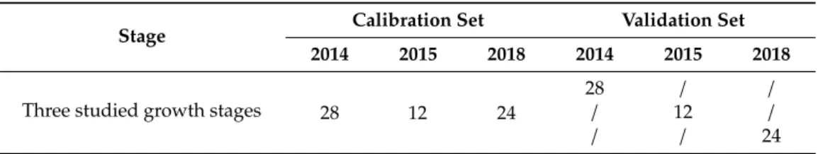
Table 3. The number of samples used in calibration and validation for the three studied growth stages. Stage Calibration Set Validation Set
2014 2015 2018 2014 2015 2018
Three studied growth stages 28 12 24
28 / /
/ 12 /
/ / 24
The slash indicates no data.
Figure 3. The distribution of region of interest (ROI) marked by the red rectangle frame. (a) Top part of the leaf; (b) middle part of the leaf; (c) bottom part of the leaf.
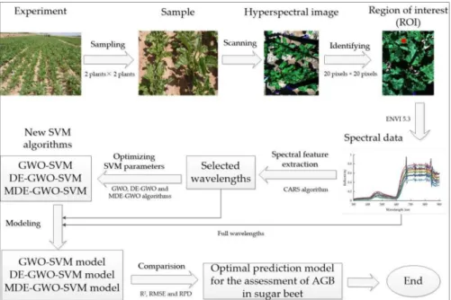
In this paper, models for the prediction of AGB were developed using both full spectra and selected wavelengths. CARS was first applied to select the most sensitive wavelengths to AGB for three growth stages. Three optimization methods of grey wolf optimization (GWO), differential evolution–GWO (DE–GWO) and modified DE–GWO (MDE–GWO) were used to optimize SVM parameters, c and γ. A support vector machine (SVM) was finally used to predict AGB using the full spectra and selected wavelengths by CARS. The main steps of the HSI prediction of AGB in sugar beet followed in this study are shown in Figure 4.
Figure 3.The distribution of region of interest (ROI) marked by the red rectangle frame. (a) Top part of the leaf; (b) middle part of the leaf; (c) bottom part of the leaf.
Table 3.The number of samples used in calibration and validation for the three studied growth stages.
Stage Calibration Set Validation Set
2014 2015 2018 2014 2015 2018
Three studied growth stages 28 12 24
28 / /
/ 12 /
/ / 24
The slash indicates no data.
In this paper, models for the prediction of AGB were developed using both full spectra and selected wavelengths. CARS was first applied to select the most sensitive wavelengths to AGB for three growth stages. Three optimization methods of grey wolf optimization (GWO), differential evolution–GWO (DE–GWO) and modified DE–GWO (MDE–GWO) were used to optimize SVM parameters, c andγ. A support vector machine (SVM) was finally used to predict AGB using the full spectra and selected wavelengths by CARS. The main steps of the HSI prediction of AGB in sugar beet followed in this study are shown in Figure4.
Remote Sens.2020,12, 620 7 of 22
Remote Sens. 2020, 12, x FOR PEER REVIEW 7 of 23
Figure 4. Main steps of above-ground biomass (AGB) prediction of sugar beet using hyperspectral imaging data.
2.3.1. Competitive Adaptive Reweighted Sampling Algorithm (CARS)
The literature shows that the utilization of all variables contained in spectra will not always result in the best prediction accuracy, despite the calculation cost. Therefore, the selection of a set of wavelength variables can not only lead to an increase in the prediction performance accuracy, but reduce the computational cost. CARS was adopted in this study to select the most significant wavelengths for AGB. It is a variable selection algorithm to imitate Darwin’s evolution theory of survival of the fittest [27]. In CARS, each wavelength variable is considered as an individual, and individuals contributing to the low prediction accuracy are gradually eliminated. During wavelength selection, the exponentially decreasing function (EDF) is utilized to remove the wavelengths having relatively small absolute regression coefficients by force. Then, adaptive reweighted sampling (ARS) is employed to further eliminate wavelengths in a competitive way and select individuals with larger absolute values of regression coefficients resulted from a partial least squares (PLS) regression model to obtain multiple subsets of wavelength variables. Eventually, according to the lowest root mean squared error of cross-validation (RMSE), an optimal subset of wavelength variables was selected as the optimal wavelengths to be used further in the analysis. More detailed information about the principle and algorithm of CARS can be found in the open literature [28].
2.3.2. Grey Wolf Optimization Algorithm (GWO)
Although SVM is one of the most efficient methods in creating reliable quantitative models for key crop properties, the accuracy, stability and generalization of SVM are determined by two parameters, penalty factor (c) and kernel parameter (γ), which change with data [16]. An optimization approach is needed to optimize these parameters with the aim of maximizing the performance of SVM. Grey wolf optimization (GWO), imitating the hierarchical mechanism (4 level hierarchy) and hunting mechanism of the grey wolf pack, is a meta-heuristic algorithm proposed by Mirjalili et al. [29], with the characteristics of providing strong convergence with fewer input parameters and can be easily realized. Like other bionic algorithms, GWO has a strict mechanism of synergy within the group. In each iteration, the leader wolves are selected through competition within the group. Under the guide of leader wolves, wolves are constantly approaching the prey and attempt to find better prey through collaborative communication. In the algorithm, the position of each grey wolf corresponds to a possible solution. The alpha (α) wolves, the leaders of the pack, are considered as the dominant solution of problems. The beta (β) wolves, the second most eligible candidates for the
Figure 4. Main steps of above-ground biomass (AGB) prediction of sugar beet using hyperspectral imaging data.
2.3.1. Competitive Adaptive Reweighted Sampling Algorithm (CARS)
The literature shows that the utilization of all variables contained in spectra will not always result in the best prediction accuracy, despite the calculation cost. Therefore, the selection of a set of wavelength variables can not only lead to an increase in the prediction performance accuracy, but reduce the computational cost. CARS was adopted in this study to select the most significant wavelengths for AGB. It is a variable selection algorithm to imitate Darwin’s evolution theory of survival of the fittest [27]. In CARS, each wavelength variable is considered as an individual, and individuals contributing to the low prediction accuracy are gradually eliminated. During wavelength selection, the exponentially decreasing function (EDF) is utilized to remove the wavelengths having relatively small absolute regression coefficients by force. Then, adaptive reweighted sampling (ARS) is employed to further eliminate wavelengths in a competitive way and select individuals with larger absolute values of regression coefficients resulted from a partial least squares (PLS) regression model to obtain multiple subsets of wavelength variables. Eventually, according to the lowest root mean squared error of cross-validation (RMSE), an optimal subset of wavelength variables was selected as the optimal wavelengths to be used further in the analysis. More detailed information about the principle and algorithm of CARS can be found in the open literature [28].
2.3.2. Grey Wolf Optimization Algorithm (GWO)
Although SVM is one of the most efficient methods in creating reliable quantitative models for key crop properties, the accuracy, stability and generalization of SVM are determined by two parameters, penalty factor (c) and kernel parameter (γ), which change with data [16]. An optimization approach is needed to optimize these parameters with the aim of maximizing the performance of SVM. Grey wolf optimization (GWO), imitating the hierarchical mechanism (4 level hierarchy) and hunting mechanism of the grey wolf pack, is a meta-heuristic algorithm proposed by Mirjalili et al. [29], with the characteristics of providing strong convergence with fewer input parameters and can be easily realized. Like other bionic algorithms, GWO has a strict mechanism of synergy within the group. In each iteration, the leader wolves are selected through competition within the group. Under the guide of leader wolves, wolves are constantly approaching the prey and attempt to find better prey through collaborative communication. In the algorithm, the position of each grey wolf corresponds to a possible solution. The alpha (α) wolves, the leaders of the pack, are considered as the dominant
Remote Sens.2020,12, 620 8 of 22
solution of problems. The beta (β) wolves, the second most eligible candidates for the position of
αand the delta (δ), who obey the orders ofαare considered as the second and third best solutions, respectively. The lowest level of grey wolves is omega (ω) wolves, whose main responsibility is to balance the internal relations of the population.
The hunting mechanism of a grey wolf pack included three successive steps of encircling, hunting and attacking. To encircle a prey, the position of each individual wolf in the pack in each iteration was modeled as detailed in Equations (3)–(7) [30]:
→ D= → C× → XP(t)− → X(t) (3) → X(T+1) = → XP(t)− → A× → D (4) → A=2×→a×→r1−→a (5) → C =2×→r2 (6) → a =2−2×t T (7)
wheretis the current iteration andTis the maximum iteration,
→
Aand
→
Care the coefficient factors,
→
XP
is the position vector of the prey,→ais linearly decreased from 2 to 0 with the lapse of iterations and the vectors,→r1and
→
r2, are random vectors in the range of [0, 1].
When hunting, GWO assumes thatα,βandδ wolves have better knowledge about the prey position. The position of the global optimal solution is estimated by the position of the current three best solutions. Therefore, other grey wolves in the pack update their positions according to the positions of α,βandδ, explained in the following equations:
→ Dα= → C1× → Xα− → X(t) (8) → Dβ= → C2× → Xβ− → X(t) (9) → Dδ= → C3× → Xδ− → X(t) (10) → X1= → Xα(t)− → A1×( → Dα) (11) → X2= → Xβ(t)− → A2×( → Dβ) (12) → X3= → Xδ(t)− → A3×( → Dδ) (13) → X(t+1) = → X1+ → X2+ → X3 3 (14)
For attacking, when|A| <1, the grey wolves attack the prey, otherwise, when|A| >1, the grey wolves will expand the region to search a prey. In this paper, the GWO algorithm was employed for parameter optimization, due to the fewer operators and parameters that need to be adjusted. The prey is the optimal value of the parameter. However, for high-dimensional or multi-objective optimization problems, the GWO algorithm is prone to fall into a local optimum with low optimization accuracy. 2.3.3. Differential Evolution Algorithm (DE)
The differential evolution (DE) algorithm, a multi-objective (continuous variable) optimization algorithm, was proposed by Storn and Price [31] on the basis of evolutionary ideas. The main idea of DE is to evolve based on individual differences. DE algorithm can be run in four successive steps
Remote Sens.2020,12, 620 9 of 22
including initialization, mutation, crossover and selection. To start with, the number of candidate solutions in the population (NP) is randomly created [32].
X0j,i=Xminj +aj× Xmaxj −Xmin j , i=1,. . .,NP, j=1,. . .,D (15) whereajis a uniformly distributed random number within the range [0, 1], regenerated for each value
ofj,Dis the dimension of each solution vector andXmaxj andXminj are the upper and lower bounds of thej-th decision parameter, respectively.
The mutation operator creates mutant vectorsXi, by perturbing a randomly selected vectorXr1with the difference of two other randomly selected vectorsXr2andXr3, according to the following equation:
X0iG=XrG1+F×XG r2−X G r3 (16) whereGis the evolutionary algebra of the population,i,r1,r2 and r3∈{1, 2,. . .,NP} are randomly chosen and must be different from each other andFis the scaling factor∈[0, 2] adjusting the perturbation vector’s size,XG
r2−XGr3, and improving algorithm convergence. The process of crossover in DE is enumerated as follow:
X00j,iG= X0G j,i randj,i(0, 1)<CR or j= jrand XGj,i otherwise (17)
whererandj,idenotes a random number within the range [0, 1], generated anew for each value of
j. The crossover constantCR, chosen from within the range [0, 1], is an algorithm parameter that
controls the diversity of the population and aids the algorithm to escape from local minima.jrandis an
integer randomly generated within the range [0, D], to ensure that the trial vector is different from the current individual.
The selection operator forms the population by choosing between the trial vectors and their predecessors (target vectors); those individuals present a better fitness or are more optimal according to Equation (18): XGi +1= X00iG i f fXi00G≤ fXG i XGi otherwise (18)
Although the DE algorithm has strong global search ability, its performance is very sensitive to parameter changes, and the local search ability is insufficient. Therefore, DE was introduced in GWO to solve the defect in this work.
2.3.4. Differential Evolution Grey Wolf Optimization Algorithm (DE–GWO)
Considering the complementarity and difference between the different intelligent optimization algorithms, a more efficient hybrid optimization algorithm, the DE–GWO algorithm, was proposed by Zhu et al. [21] to solve the premature problem and improve the overall search capability of GWO. DE is used to maintain the diversity of the grey wolf population to avoid the reduction of population differences during iteration. The mathematical model of DE–GWO can be described in six steps as follows:
Step 1: Initialization: After repeated attempts, initial parameter values of DE–GWO were determined. The size of initial population of DE–GWO was 30, and maximum iteration was 500. The dimension of independent variables was 2. The upper and lower bounds of scaling factors were set to be 0.8 and 0.2, respectively, and the crossover probability was 0.2; upper and lower bounds of parameter values were 0.01 and 100, respectively. This was followed by setting the initial values of the parameters a, A and C and randomly generating the initial positions of the population individuals using Equation (15).
Step 2: Perform mutation operations on individual populations to produce variable populations using Equation (16) and then generate the initial parent population through the selection operation of DE using Equation (18).
Remote Sens.2020,12, 620 10 of 22
Step 3: Calculate the objective function value of each grey wolf individual in the population using Equation (19). According to the size of the objective function value, the first three individuals with the lowest fitness value were selected, and then they were recorded asXα, Xβ, Xδin ascending order.
f itnessi= fRMSE(SVM) (19)
wherefRMSE(·) is the function to calculate the root mean squared error (RMSE) of SVM.
Step 4: Calculate the distance between other grey wolf individuals in the population and the optimalXα, Xβ, Xδ, using Equations (8)–(10), and update the position of each grey wolf individually using Equations (11)–(14).
Step 5: Update the values of A, C and a using Equations (5)–(7). Based on the intermediate population generated by the mutation operation of DE, the progeny population was created by the cross operation. Then, the parent population is updated by the selection process of DE.
Step 6: Calculate the fitness value of all grey wolf individuals, and update the positions ofXα, Xβ, Xδof the parent population according to the size of the fitness value.
Step 7: Determine whether the maximum number of iterations was reached. If yes, exit the optimization and return the value ofXαas the final optimal solution, otherwise, go back to Step 2 to continue.
2.3.5. Modified Differential Evolution Grey Wolf Optimization Algorithm (MDE–GWO)
Compared to GWO and DE, the defection of the Local optimum can be solved and the global search ability can be improved by the DE–GWO algorithm. However, higher prediction accuracy and faster convergence speed could be achieved, only when the global exploration and local exploitation are in a good balance. According to the GWO algorithm, the relationship between the absolute value of A and 1 determines if the algorithm will perform the local exploitation or global exploration. Nevertheless, the A value is changed with the convergence factor (a) as explained in Equation (5), which means a is the direct influencing factor of the balance between global exploration and local exploitation in DE–GWO. In general, a is set to decrease linearly from 2 to 0 as iteration increases. However, in practice, the actual iterative search process of the GWO algorithm is non-linear. Therefore, the linear decreasing tendency of a cannot accurately reflect the actual cooperative hunting process of the grey wolf pack. To obtain more accurate optimization results, a novel modified algorithm of the DE–GWO algorithm (MDE–GWO) was proposed in this paper. To balance the ability of global exploration and local exploitation, a novel formula for calculating a based on a cosine function and an exponential function was developed (Equation (20)). It helps DE–GWO to alter the search space according to the non-linear variations by searching quickly in a large area at first and then attacking slowly in a small space.
a= 1
−9×coset/T−1
5 (20)
wheretis the iteration andTis the maximum iteration. 2.3.6. Support Vector Machines Algorithm (SVM)
The SVM is a linear data processing method derived from statistical learning theory, which is originally introduced by Cortes and Vapnik [33], based on the principle of structural risk minimization. However, the introduction of kernel methods is the pivotal part for SVM to solve the contradiction between high dimension and the computational complexity of samples. An SVM is described as a quadratic optimization problem [33]:
min w,b,ξ 1 2kwk 2+c N X i=1 ξi (21)
Remote Sens.2020,12, 620 11 of 22
wherewis the optimal solution andbis the bias parameter,c>0 is the penalty parameter of the error term andξiis called the slack variable that is related to prediction errors in SVM.
The formation and function of SVM are determined by the type of kernel function used. Polynomial, radial basis functions (RBF) and sigmoid (two-layer neural networks) are the most commonly used kernel functions for the nonlinear data. Due to small computational cost, high prediction accuracy and good stability, the RBF was used in this paper, which can be written as follows [34]:
K(xi,xj) =exp(−γkxi−xjk2),γ >0 (22)
whereγis the width parameter of RBF function.
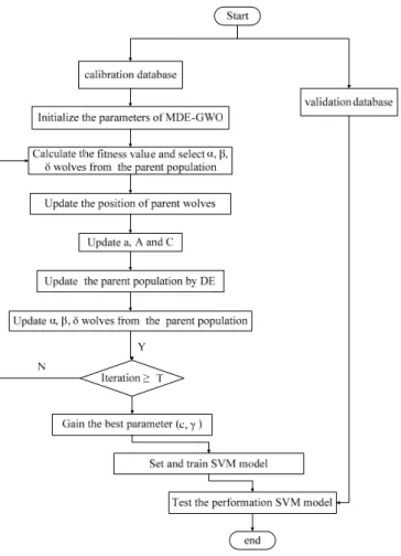
The values of c andγare very critical and affect the prediction accuracy of SVM. The selection of correct values will result in high prediction accuracies and reduce the processing time. They should be determined prior to the training stage. Therefore, to get an accurate prediction result for AGB in sugar beet by the SVM model, the penalty factor, c, and the kernel parameter,γ, were taken as the base 2 indexes and GWO, DE–GWO and MDE–GWO were employed to optimize them in this paper. Prediction models of GWO–SVM, DE–GWO–SVM and MDE–GWO–SVM were constructed in Matlab R2014a software. The flowchart of MDE–GWO–SVM is shown in Figure5, as an example. The performance of SVM prediction models was compared by means of the coefficient of determination (R2), the root mean squared error (RMSE) and the ratio of prediction deviation (RPD), which is the standard deviation of measured AGB divided by RMSE. The higher the R2and RPD values and the lower the RMSE values, the better the model prediction performance.
Remote Sens. 2020, 12, x FOR PEER REVIEW 11 of 23
where γ is the width parameter of RBF function.
The values of c and γ are very critical and affect the prediction accuracy of SVM. The selection of correct values will result in high prediction accuracies and reduce the processing time. They should be determined prior to the training stage. Therefore, to get an accurate prediction result for AGB in sugar beet by the SVM model, the penalty factor, c, and the kernel parameter, γ, were taken as the base 2 indexes and GWO, DE–GWO and MDE–GWO were employed to optimize them in this paper. Prediction models of GWO–SVM, DE–GWO–SVM and MDE–GWO–SVM were constructed in Matlab R2014a software. The flowchart of MDE–GWO–SVM is shown in Figure 5, as an example. The performance of SVM prediction models was compared by means of the coefficient of determination (R2), the root mean squared error (RMSE) and the ratio of prediction deviation (RPD), which is the
standard deviation of measured AGB divided by RMSE. The higher the R2 and RPD values and the
lower the RMSE values, the better the model prediction performance.
Figure 5. Flow chart of modified differential evolution grey wolf optimization (MDE–GWO–SVM) algorithm.
3. Results
3.1. Above-Ground Biomass (AGB) Variability
Table 4 summarizes the measurement results of AGB during each growth stage for the calibration and validation datasets. For the calibration set, AGB varies from 33.47 to 596.95 g/m2 in
the rapid growth stage of leaf cluster, 82.64 to 1012.04 g/m2 in the sugar growth stage and 138.54 to
789.77 g/m2 in the sugar accumulation stage. The sugar growth stage has the highest mean value of
AGB of 530.25 g/m2 than the other two stages. For the validation dataset, the ranges of AGB of each
year are smaller and within the range of the corresponding calibration dataset. This is important as if the range of variability in the validation set is larger than that of the calibration set, prediction
Figure 5. Flow chart of modified differential evolution grey wolf optimization (MDE–GWO–SVM) algorithm.
Remote Sens.2020,12, 620 12 of 22
3. Results
3.1. Above-Ground Biomass (AGB) Variability
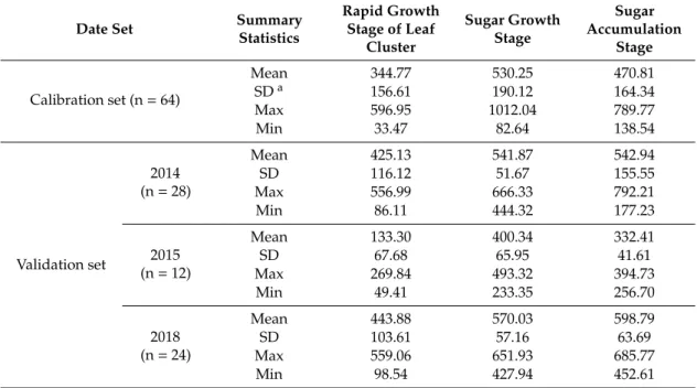
Table4summarizes the measurement results of AGB during each growth stage for the calibration and validation datasets. For the calibration set, AGB varies from 33.47 to 596.95 g/m2in the rapid growth stage of leaf cluster, 82.64 to 1012.04 g/m2in the sugar growth stage and 138.54 to 789.77 g/m2 in the sugar accumulation stage. The sugar growth stage has the highest mean value of AGB of 530.25 g/m2than the other two stages. For the validation dataset, the ranges of AGB of each year are smaller and within the range of the corresponding calibration dataset. This is important as if the range of variability in the validation set is larger than that of the calibration set, prediction accuracy might deteriorate due to the smaller range of variability accounted for in the calibration stage [35,36].
Table 4.Above-ground biomass (AGB) range in g/m2shown for each growth stage.
Date Set Summary
Statistics Rapid Growth Stage of Leaf Cluster Sugar Growth Stage Sugar Accumulation Stage Calibration set (n=64) Mean 344.77 530.25 470.81 SDa 156.61 190.12 164.34 Max 596.95 1012.04 789.77 Min 33.47 82.64 138.54 Validation set 2014 (n=28) Mean 425.13 541.87 542.94 SD 116.12 51.67 155.55 Max 556.99 666.33 792.21 Min 86.11 444.32 177.23 2015 (n=12) Mean 133.30 400.34 332.41 SD 67.68 65.95 41.61 Max 269.84 493.32 394.73 Min 49.41 233.35 256.70 2018 (n=24) Mean 443.88 570.03 598.79 SD 103.61 57.16 63.69 Max 559.06 651.93 685.77 Min 98.54 427.94 452.61 aStandard deviation.
3.2. Correlation between Above-Ground Biomass (AGB) and Canopy Reflectance Wavelength
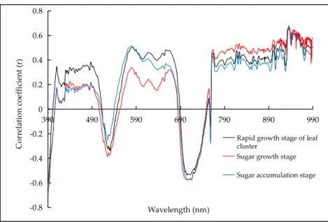
Considerably similar patterns of Pearson correlation coefficients (r) between AGB and wavelengths can be clearly observed across the entire spectral range (Figure6) for the three studied growth stages. However, large differences in correlation coefficients among growth stages are observed particularly at wavebands in the visible range of 390–410 nm (blue), 570–584 nm (green), 660–680 nm (red) and 700–710 nm (red-edge) and 936–960 nm in the near-infrared spectral range. Similar results were reported by Hansen et al. [11] and Nguyen et al. [5] for wheat and rice, respectively. Therefore, these peak differences can be attributed to differences in AGB content, hence, the potential for successful AGB prediction with HSI. The large differences in raw reflectance at these wavebands (data not shown) are in agreement with the reasonable linear correlations between AGB and reflectance with r value ranges of−0.7–0.33, 0.37–0.49, 0.42–0.58,−0.57–−0.53 and 0.49–0.67 for blue, green, red, red-edge and near-infrared bands, respectively. Moreover, due to the high dimensionality and collinearity of the three-dimensional HSI data, the correlation between adjacent wavelengths and AGB is almost identical and does not clearly differ among different adjacent wavelengths within a certain range, such as 870 nm to 890 nm. Besides, the highest correlation coefficient value was less than 0.7, illustrating that information from a single-band is not enough to predict AGB of sugar beet successfully and that
Remote Sens.2020,12, 620 13 of 22
several selected wavelengths or the full spectral data are necessary. Therefore, the potential of the variable selection algorithm is investigated in the following section.Remote Sens. 2020, 12, x FOR PEER REVIEW 13 of 23
Figure 6. The Pearson correlation coefficients (r) between the spectral wavelengths and the measured above-ground biomass (AGB).
3.3. Characteristic Wavelengths Selection with Competitive Adaptive Reweighted Sampling (CARS)
As shown in Figure 7, with the increasing number of sampling runs from 0 to 50, different patterns of changes in the number of sampled variable (wavelengths), root mean square error of cross-validation (RMSE) obtained from the PLS regression analysis and the regression coefficients path can be observed, and the pattern of changes varies among the three studied growth stages. Variation in the number of sampled wavelength shows a two-phase selection, namely, fast selection and refined (fine-tuned) selection. In the fast selection stage, due to the EDF, the number of sampled variables dropped rapidly in the early stage of sampling runs. Then, with the increase of sampling runs, ARS was used to select the key variables based on the regression coefficients. Therefore, after the second sampling run, the number of sampled variables was decreased cautiously in the refined selection until the optimal subset was obtained. The RMSE values of 10-fold cross-validation have not changed in the sampling runs 1–18 (rapid growth stage of leaf cluster and sugar growth stage) and 1–17 (sugar accumulation stage) because of the presence of uninformative variables. Then, RMSE values decreased in sampling runs 19–31 (rapid growth stage of leaf cluster), 19–30 (sugar growth stage) and 18–31 (sugar accumulation stage), indicating that redundant variables that are uncorrelated with AGB were excluded. The minimal RMSE value of three growth stages was located at the sampling runs 31, 30 and 31 for the rapid growth stage of leaf cluster, sugar growth stage and sugar accumulation stage, respectively. These minimal RMSE values marked by a blue asterisk line in Figure 7 were used to determine the optimal variable subset. After the sampling runs of minimal RMSE, some key variables for AGB prediction were culled, resulting in larger residuals, hence, the RMSE values increased, and reached larger maximum values than those at the start of the sampling runs.
CARS algorithm reduced the number of wavelengths considerably from the original 823 to 21 variables for both the rapid growth stage of leaf cluster and sugar accumulation stage and 23 for the sugar growth stage. These wavelengths are predominately located at eight distinctive wavebands centering at 410, 674, 715, 751, 833, 893, 940 and 971 nm (Figure 8). These selected wavelengths were then used for SVM modeling, whose results are compared to those of SVM models developed with the full spectrum.
-0.8 -0.6 -0.4 -0.2 0 0.2 0.4 0.6 0.8 390 490 590 690 790 890 990 Co rrelatio n coeff icient ( r) Wavelength (nm)
Rapid growth stage of leaf cluster
Sugar growth stage Sugar accumulation stage
Figure 6.The Pearson correlation coefficients (r) between the spectral wavelengths and the measured above-ground biomass (AGB).
3.3. Characteristic Wavelengths Selection with Competitive Adaptive Reweighted Sampling (CARS)
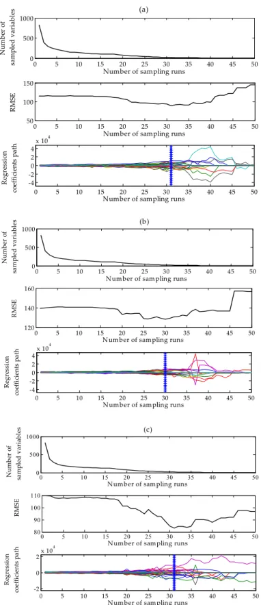
As shown in Figure7, with the increasing number of sampling runs from 0 to 50, different patterns of changes in the number of sampled variable (wavelengths), root mean square error of cross-validation (RMSE) obtained from the PLS regression analysis and the regression coefficients path can be observed, and the pattern of changes varies among the three studied growth stages. Variation in the number of sampled wavelength shows a two-phase selection, namely, fast selection and refined (fine-tuned) selection. In the fast selection stage, due to the EDF, the number of sampled variables dropped rapidly in the early stage of sampling runs. Then, with the increase of sampling runs, ARS was used to select the key variables based on the regression coefficients. Therefore, after the second sampling run, the number of sampled variables was decreased cautiously in the refined selection until the optimal subset was obtained. The RMSE values of 10-fold cross-validation have not changed in the sampling runs 1–18 (rapid growth stage of leaf cluster and sugar growth stage) and 1–17 (sugar accumulation stage) because of the presence of uninformative variables. Then, RMSE values decreased in sampling runs 19–31 (rapid growth stage of leaf cluster), 19–30 (sugar growth stage) and 18–31 (sugar accumulation stage), indicating that redundant variables that are uncorrelated with AGB were excluded. The minimal RMSE value of three growth stages was located at the sampling runs 31, 30 and 31 for the rapid growth stage of leaf cluster, sugar growth stage and sugar accumulation stage, respectively. These minimal RMSE values marked by a blue asterisk line in Figure7were used to determine the optimal variable subset. After the sampling runs of minimal RMSE, some key variables for AGB prediction were culled, resulting in larger residuals, hence, the RMSE values increased, and reached larger maximum values than those at the start of the sampling runs.
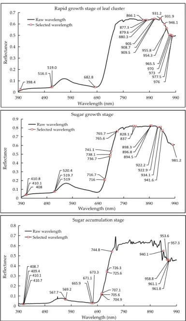
CARS algorithm reduced the number of wavelengths considerably from the original 823 to 21 variables for both the rapid growth stage of leaf cluster and sugar accumulation stage and 23 for the sugar growth stage. These wavelengths are predominately located at eight distinctive wavebands centering at 410, 674, 715, 751, 833, 893, 940 and 971 nm (Figure8). These selected wavelengths were then used for SVM modeling, whose results are compared to those of SVM models developed with the full spectrum.
Remote Sens.Remote Sens. 20202020,, 12, x FOR PEER REVIEW 12, 620 14 of 2214 of 23
Figure 7. The wavelength selection results obtained from competitive adaptive reweighted sampling (CARS) in (a) rapid growth stage of leaf cluster, (b) sugar growth stage and (c) sugar accumulation stage, shown as changes in the number of selected variables, root mean square error of cross-validation (RMSE) and the regression coefficients path of each variable (different colored lines refer to the regression coefficient of each wavelength).
0 5 10 15 20 25 30 35 40 45 50
0 500 1000
Number of sampling runs
Nu mb er o f sa m p le d v a ri a b le s 0 5 10 15 20 25 30 35 40 45 50 50 100 150
Number of sampling runs
RM S E 0 5 10 15 20 25 30 35 40 45 50 -4 -2 0 2 4 x 10⁴
Number of sampling runs
R egre ss io n co ef fi ci en ts p a th (a) 0 5 10 15 20 25 30 35 40 45 50 0 500 1000
N um ber of sam pling runs
N u mb er o f sa m p le d v a ri a b le s 0 5 10 15 20 25 30 35 40 45 50 120 140 160
Num ber of sampling runs
RMS E 0 5 10 15 20 25 30 35 40 45 50 -4 -2 0 2 4 x 10⁴
Number of sam pling runs
R egr es si o n co eff ic ien ts p a th (b) 0 5 10 15 20 25 30 35 40 45 50 0 500 1000
N um ber of sam pling runs
N u m b er o f sa m p le d v a riab le s 0 5 10 15 20 25 30 35 40 45 50 80 90 100 110
N um ber of sam pling runs
RM S E 0 5 10 15 20 25 30 35 40 45 50 -2 0 2x 10 4
N um ber of sam pling runs
R egr es si o n coe ff ici en ts pa th (c)
Figure 7.The wavelength selection results obtained from competitive adaptive reweighted sampling (CARS) in (a) rapid growth stage of leaf cluster, (b) sugar growth stage and (c) sugar accumulation stage, shown as changes in the number of selected variables, root mean square error of cross-validation (RMSE) and the regression coefficients path of each variable (different colored lines refer to the regression coefficient of each wavelength).
Remote Sens.2020,12, 620 15 of 22
Remote Sens. 2020, 12, x FOR PEER REVIEW 15 of 23
Figure 8. The selected key wavelengths marked by a square for the three studies growth stages, resulted from competitive adaptive reweighted sampling algorithm (CARS).
3.4. Modified Differential Evolution Grey Wolf Optimization (MDE–GWO)
The fitness value convergence curve during the iteration carried out for DE–GWO and MDE– GWO is shown in Figure 9. The curve for the MDE–GWO algorithm shows rapid and higher convergence accuracy, compared to the DE–GWO algorithm. Converge began with a minimum fitness value of 17.93 and 17.82 after iterations of 130 and 70 for DE–GWO and MDE–GWO, respectively. Due to the dynamic adjustment of the convergence factor (Ia) with the increasing iteration, the convergence speed is improved, with significant improvement in the accuracy of optimization, evaluated as RMSE. Therefore, the proposed MDE–GWO algorithm was chosen as the best method for optimizing the SVM performance for the prediction of AGB of sugar beet with less computational effort and higher accuracy.
954.3 955.8 398.4 965.5 970 973 976 977.5 866.1 682.8 877.3 879.6 880.3 516.8 519.0 905 908.7 909.5 931.2 931.9 946.1 0 0.1 0.2 0.3 0.4 0.5 0.6 0.7 390 490 590 690 790 890 990 Re fl ec ta nce Wavelength (nm) Rapid growth stage of leaf cluster
Raw wavelength Selected wavelength 765.7 765.6 408 410.1 410.8 981.2 828.1 837 894.5 519 519.7 520.4 896.8 898.3 716 716.7 922.2 922.9 736.7 738.1 741.1 934.1 941.6 0 0.1 0.2 0.3 0.4 0.5 0.6 0.7 0.8 0.9 390 490 590 690 790 890 990 Re fl ec ta nc e Wavelength (nm) Sugar growth stage Raw wavelength Selected wavelength 953.6 957.3 958.8 961.1 961.8 408.7 409.4 410.1 410.7 665.9 671.1 673.3 705.6 704.9 707.1 725.6 726.3 744.8 940.1 567.7 569.2 0 0.1 0.2 0.3 0.4 0.5 0.6 0.7 0.8 390 490 590 690 790 890 990 Re fl ec ta nce Wavelength (nm) Sugar accumulation stage Raw wavelength
Selected wavelength
Figure 8.The selected key wavelengths marked by a square for the three studies growth stages, resulted from competitive adaptive reweighted sampling algorithm (CARS).
3.4. Modified Differential Evolution Grey Wolf Optimization (MDE–GWO)
The fitness value convergence curve during the iteration carried out for DE–GWO and MDE–GWO is shown in Figure9. The curve for the MDE–GWO algorithm shows rapid and higher convergence accuracy, compared to the DE–GWO algorithm. Converge began with a minimum fitness value of 17.93 and 17.82 after iterations of 130 and 70 for DE–GWO and MDE–GWO, respectively. Due to the dynamic adjustment of the convergence factor (Ia) with the increasing iteration, the convergence speed is improved, with significant improvement in the accuracy of optimization, evaluated as RMSE. Therefore, the proposed MDE–GWO algorithm was chosen as the best method for optimizing the SVM performance for the prediction of AGB of sugar beet with less computational effort and higher accuracy.
Remote Sens.2020,12, 620 16 of 22
Remote Sens. 2020, 12, x FOR PEER REVIEW 16 of 23
Figure 9. Fitness value convergence curve shown for differential evolution grey wolf optimization (DE–GWO) (a) and modified differential evolution grey wolf optimization (MDE–GWO) (b) algorithms.
3.5. Support Vector Machine (SVM) Models for Above-Ground Biomass (AGB) Prediction
Using the selected characteristic wavelength variables shown in Figure 8, quantitative prediction models (GWO–SVM, DE–GWO–SVM and MDE–GWO–SVM) for AGB of sugar beet were established. In order to evaluate the performance of models with selected wavelengths by CARS, corresponding models using the full wavelengths were also developed. The performance of these prediction models is illustrated in Table 5. Surprisingly, almost all models with the wavelengths selected by CARS performed better than those developed with the full wavelength range, with improvement in % R2
and RPD values of 2.8–50% and 5.6–164%, respectively, and decreases in RMSE values by 18.6–28% for the validation set.
In terms of model prediction accuracy, it can be observed in Table 5 that different optimization algorithms have different effects on the performance of SVM models. Overall, the accuracy of SVM models was affected by the optimization algorithms. The best results were achieved by employing the MDE–GWO algorithm to optimize the two parameters of SVM, c and γ, followed successively by DE–GWO and GWO algorithms. For MDE–GWO–SVM models with selected wavelengths, R2 values
of the validation set were 0.80, 0.74 and 0.75, with RMSE values of 53.69, 46.17 and 65.68 g/m2, and
RPD values of 1.97, 1.42 and 1.71, respectively, for 2014, 2015 and 2018 in the rapid growth stage of leaf cluster. In the sugar growth stage, the best prediction results were obtained compared with the other two growth stages, with R2 values of the validation set of 0.80, 0.78 and 0.80, RMSE values of
30.16, 32.35 and 37.03 g/m2 and RPD values of 2.03, 1.97 and 1.69, respectively. In the sugar
accumulation stage, the poorest prediction results of AGB were recorded with R2 values of the
validation set of 0.73, 0.69 and 0.74, RMSE values of 104.08, 40.77 and 40.17 g/m2, and RPD values of
1.72, 1.61 and 1.95, respectively. Therefore, the MDE–GWO algorithm is deemed to be the best among the three methods for parameter optimization of SVM in this paper, and the convergence factor calculated by the proposed MDE–GWO algorithm is more suitable in this case than those obtained with GWO or DE–GWO algorithms.
Figure 10 illustrates scatter plots of the measured versus predicted AGB values of the validation set in 2014 for different models (CARS–GWO–SVM, CARS–DE–GWO–SVM and CARS–MDE–GWO– SVM), shown for the sugar growth stage, as an example. The majority of predicted values are distributed closely around the 1:1 regression line. The smallest slop is calculated for the linear regression line for the MDE–GWO–SVM model, indicating the smallest under- or over-prediction error. This shows that the newly-developed MDE–GWO–SVM model in this study is a promising tool for the prediction of AGB in sugar beet with high accuracy.
17.8 17.9 18.0 18.1 18.2 18.3 18.4 18.5 0 50 100 150 200 250 300 350 400 450 500 Fitt ness v alue Iteration (a) 17.8 17.9 18.0 18.1 18.2 18.3 18.4 18.5 0 50 100 150 200 250 300 350 400 450 500 Fi tt n es s v alue Iteration (b)
Figure 9. Fitness value convergence curve shown for differential evolution grey wolf optimization (DE–GWO) (a) and modified differential evolution grey wolf optimization (MDE–GWO) (b) algorithms. 3.5. Support Vector Machine (SVM) Models for Above-Ground Biomass (AGB) Prediction
Using the selected characteristic wavelength variables shown in Figure8, quantitative prediction models (GWO–SVM, DE–GWO–SVM and MDE–GWO–SVM) for AGB of sugar beet were established. In order to evaluate the performance of models with selected wavelengths by CARS, corresponding models using the full wavelengths were also developed. The performance of these prediction models is illustrated in Table5. Surprisingly, almost all models with the wavelengths selected by CARS performed better than those developed with the full wavelength range, with improvement in % R2and RPD values of 2.8–50% and 5.6–164%, respectively, and decreases in RMSE values by 18.6–28% for the validation set.
In terms of model prediction accuracy, it can be observed in Table5that different optimization algorithms have different effects on the performance of SVM models. Overall, the accuracy of SVM models was affected by the optimization algorithms. The best results were achieved by employing the MDE–GWO algorithm to optimize the two parameters of SVM, c andγ, followed successively by DE–GWO and GWO algorithms. For MDE–GWO–SVM models with selected wavelengths, R2values of the validation set were 0.80, 0.74 and 0.75, with RMSE values of 53.69, 46.17 and 65.68 g/m2, and RPD values of 1.97, 1.42 and 1.71, respectively, for 2014, 2015 and 2018 in the rapid growth stage of leaf cluster. In the sugar growth stage, the best prediction results were obtained compared with the other two growth stages, with R2values of the validation set of 0.80, 0.78 and 0.80, RMSE values of 30.16, 32.35 and 37.03 g/m2and RPD values of 2.03, 1.97 and 1.69, respectively. In the sugar accumulation stage, the poorest prediction results of AGB were recorded with R2values of the validation set of 0.73, 0.69 and 0.74, RMSE values of 104.08, 40.77 and 40.17 g/m2, and RPD values of 1.72, 1.61 and 1.95, respectively. Therefore, the MDE–GWO algorithm is deemed to be the best among the three methods for parameter optimization of SVM in this paper, and the convergence factor calculated by the proposed MDE–GWO algorithm is more suitable in this case than those obtained with GWO or DE–GWO algorithms.
Figure10illustrates scatter plots of the measured versus predicted AGB values of the validation set in 2014 for different models (CARS–GWO–SVM, CARS–DE–GWO–SVM and CARS–MDE–GWO–SVM), shown for the sugar growth stage, as an example. The majority of predicted values are distributed closely around the 1:1 regression line. The smallest slop is calculated for the linear regression line for the MDE–GWO–SVM model, indicating the smallest under- or over-prediction error. This shows that the newly-developed MDE–GWO–SVM model in this study is a promising tool for the prediction of AGB in sugar beet with high accuracy.
Remote Sens.2020,12, 620 17 of 22
Table 5.The results of support vector machine (SVM) prediction of above-ground biomass (AGB) for each growth stage, after grey wolf optimization (GWO), differential evolution grey wolf optimization (DE–GWO) and modified differential evolution grey wolf optimization (MDE–GWO) algorithms.
Growth Stages Inputs Model Calibration Set Validation Set
R2 a RMSEb (g/m2) Year R 2 RMSE (g/m2) RPDc Rapid Growth Stage of Leaf Cluster All Bands GWO 0.76 79.69 2014 0.61 82.82 0.99 2015 0.60 59.70 0.77 2018 0.70 71.79 0.81 DE–GWO 0.82 113.16 2014 0.80 58.54 1.52 2015 0.61 53.30 1.16 2018 0.70 70.65 0.82 MDE–GWO 0.86 61.41 2014 0.84 59.26 1.97 2015 0.64 49.73 1.21 2018 0.75 72.98 0.90 CARS GWO 0.78 76.84 2014 0.71 84.25 1.35 2015 0.64 42.83 1.27 2018 0.70 80.26 1.25 DE–GWO 0.82 70.73 2014 0.77 70.89 1.64 2015 0.68 46.21 1.36 2018 0.74 67.01 1.26 MDE–GWO 0.84 67.54 2014 0.80 53.69 1.97 2015 0.74 46.17 1.42 2018 0.75 65.68 1.71 Sugar Growth Stage All Bands GWO 0.78 119.66 2014 0.69 37.56 1.11 2015 0.52 70.47 1.15 2018 0.49 47.53 0.96 DE–GWO 0.82 116.94 2014 0.71 30.92 1.33 2015 0.58 67.81 1.17 2018 0.52 40.06 1.03 MDE–GWO 0.89 81.27 2014 0.82 27.66 2.01 2015 0.69 47.13 1.21 2018 0.69 35.60 1.40 CARS GWO 0.80 156.81 2014 0.75 39.68 1.47 2015 0.65 52.55 1.28 2018 0.74 46.29 1.25 DE–GWO 0.82 154.77 2014 0.77 32.13 1.60 2015 0.72 57.46 1.38 2018 0.78 66.58 0.27 MDE–GWO 0.85 154.43 2014 0.80 30.16 2.03 2015 0.78 32.35 1.97 2018 0.80 37.03 1.69 Sugar Accumulation Stage All Bands GWO 0.75 89.07 2014 0.70 99.75 1.14 2015 0.42 34.44 0.56 2018 0.70 40.14 1.10 DE–GWO 0.81 77.13 2014 0.69 94.10 1.31 2015 0.58 36.87 0.92 2018 0.71 34.89 1.60 MDE–GWO 0.83 69.83 2014 0.74 81.86 1.61 2015 0.61 27.24 1.32 2018 0.74 32.52 1.65 CARS GWO 0.80 78.87 2014 0.71 101.45 1.12 2015 0.65 25.78 1.48 2018 0.69 40.04 1.67 DE–GWO 0.82 72.27 2014 0.70 87.89 1.71 2015 0.67 30.05 1.56 2018 0.72 36.75 1.70 MDE–GWO 0.83 72.00 2014 0.73 104.08 1.72 2015 0.69 40.77 1.61 2018 0.74 40.17 1.95