Epigraphical Projection and Proximal Tools for Solving
Constrained Convex Optimization Problems: Part I
Giovanni Chierchia, Nelly Pustelnik, Jean-Christophe Pesquet, B´
eatrice
Pesquet-Popescu
To cite this version:
Giovanni Chierchia, Nelly Pustelnik, Jean-Christophe Pesquet, B´
eatrice Pesquet-Popescu.
Epi-graphical Projection and Proximal Tools for Solving Constrained Convex Optimization
Prob-lems: Part I. 2012.
<
hal-00744603v2
>
HAL Id: hal-00744603
https://hal.archives-ouvertes.fr/hal-00744603v2
Submitted on 15 Nov 2012
HAL
is a multi-disciplinary open access
archive for the deposit and dissemination of
sci-entific research documents, whether they are
pub-lished or not.
The documents may come from
teaching and research institutions in France or
abroad, or from public or private research centers.
L’archive ouverte pluridisciplinaire
HAL
, est
destin´
ee au d´
epˆ
ot et `
a la diffusion de documents
scientifiques de niveau recherche, publi´
es ou non,
´
emanant des ´
etablissements d’enseignement et de
recherche fran¸
cais ou ´
etrangers, des laboratoires
publics ou priv´
es.
Epigraphical Projection and Proximal Tools for Solving
Constrained Convex Optimization Problems: Part I
Giovanni Chierchia
∗, Nelly Pustelnik
†,
Jean-Christophe Pesquet
‡, and B´
eatrice Pesquet-Popescu
∗November 15, 2012
Abstract
We propose a proximal approach to deal with convex optimization problems involving nonlinear constraints. A large family of such constraints, proven to be effective in the solution of inverse problems, can be expressed as the lower level set of a sum of convex functions evaluated over different, but possibly overlapping, blocks of the signal. For this class of constraints, the associated projection operator generally does not have a closed form. We circumvent this difficulty by splitting the lower level set into as many epigraphs as functions involved in the sum. A closed half-space constraint is also enforced, in order to limit the sum of the introduced epigraphical variables to the upper bound of the original lower level set.
In this paper, we focus on a family of constraints involving linear transforms ofℓ1,pballs. Our main
theoretical contribution is to provide closed form expressions of the epigraphical projections associated with the Euclidean norm (p= 2) and the sup norm (p= +∞). The proposed approach is validated in the context of image restoration with missing samples, by making use of TV-like constraints. Experiments show that our method leads to significant improvements in term of convergence speed over existing algorithms for solving similar constrained problems.
1
Introduction
As an offspring of the wide interest in frame representations and sparsity promoting techniques for data recovery, there has been an emergence of proximal methods to efficiently solve convex optimization problems arising in inverse problems. Examples of applications of these methods can be found in f-MRI reconstruction [1, 2], satellite image restoration [3, 4], microscopy image deconvolution [5, 6], computed tomography [7], Positron Emission Tomography [8, 9], texture-geometry decomposition [10, 11, 12], machine learning [13, 14], stereo vision [15], and audio processing [16, 17]. Proximal algorithms have gained much popularity in solving large-size optimization problems involving non-differentiable (or even non finite) functions. One of the main advantages of these methods is that they are amenable to parallel implementations. For a survey on proximal algorithms and their applications, the reader is referred to [18, 13]. Note also that some of these methods
∗G. Chierchia (Corresponding author) and B. Pesquet-Popescu are with T´el´ecom ParisTech/Institut T´el´ecom, LTCI, UMR
CNRS 5141, 75014 Paris, France (e-mail: [email protected]).
†N. Pustelnik is with ENS Lyon, Laboratoire de Physique, UMR CNRS 5672, F69007 Lyon, France (e-mail:
‡J.-C. Pesquet is with Universit´e Paris-Est, LIGM, UMR CNRS 8049, 77454 Marne-la-Vall´ee, France (e-mail:
are closely related to augmented Lagrangian approaches [19, 20, 21]. Even if proximal algorithms and the associated convergence properties have been deeply investigated [22, 23, 24, 25], some questions persist in their use for solving inverse problems. A first question is: how can we set the parameters serving to enforce the regularity of the solution in an automatic way? Another question is related to the selection of the most appropriate algorithm within the class of proximal algorithms for a given application. This also raises the question of the computation of the proximity operators associated with the different functions involved in the criterion. Various strategies were proposed in order to address the first question [26, 27, 28, 29, 30], but the computational cost of these methods is often high, especially when several regularization parameters have to be set. Alternatively, it has been recognized for a long time that incorporating constraints directly on the solutions [31, 32, 33, 34, 35] instead of considering regularized functions may often facilitate the choice of the involved parameters. Indeed, in a constrained formulation, the constraint bounds are usually related to some physical properties of the target solution or some knowledge of the degradation process, e.g. the noise statistical properties. Note also that there exist some conceptual Lagrangian equivalences between regularized solutions to inverse problems and constrained ones, although some caution should be taken when the regularization functions are nonsmooth (see [36] where the case of a single regularization parameter is investigated).
In this context, the objective of this paper is to provide an answer to the second question, that is to propose efficient parallel algorithms for solving the following constrained convex optimization problem:
Problem 1.1. minimize x∈H R X r=1 gr(Trx) s.t. H1x∈C1, .. . HSx∈CS, (1) where
(i) for everyr∈ {1, . . . , R},Tris a bounded linear operator from a real Hilbert spaceHtoRNr;
(ii) for everyr∈ {1, . . . , R},gr is a proper lower-semicontinuous convex function fromRNr to ]−∞,+∞];
(iii) for everys∈ {1, . . . , S},Hsis a bounded linear operator fromHtoRMs;
(iv) for everys∈ {1, . . . , S},Cs is a nonempty closed convex subset ofRMs.
A large number of inverse problems can be formulated under the form of Problem 1.1. A classical application example is image recovery from blurred and noisy observations. Let z denote the vector of observed data. When the noise is assumed to be zero-mean additive white Gaussian, the restored data can be obtained by solving Problem 1.1 where R= 2, S = 0, g1 =λk · k1 withλ∈]0,+∞[, T1 is an analysis
frame operator [37] allowing us to sparsify signal x, g2 =k · −zk2, and T2 denotes the matrix associated
with the degradation blur [38, 23]. On the other hand, a constrained formulation of the same restoration problem leads to Problem 1.1 withR= 1,S = 1,g1 =k · k1,T1 is the same frame operator as previously,
and
(∀x∈ H) H1x∈C1 ⇔ kH1x−zk2≤η1.
Here,H1 denotes the matrix associated with the degradation blur, and η1 is a positive constant which is
typically chosen proportional to the noise variance. This specific constraint formulation has been considered in [39].
The present work aims at designing efficient methods in order to deal with Problem 1.1 when the convex constraints are expressed as follows: for everys∈ {1, . . . , S},
whereηs∈Randhsis a proper lower-semicontinuous function fromRMs to ]−∞,+∞].
The paper is organized as follows. In Section 2, we motivate the choice of proximal tools and recall some of their theoretical properties. In addition, closed form expressions for specific proximity operators are derived. Then, in order to deal with a constraint expressed under the general form (2), a splitting approach involving an epigraphical projection is proposed. This epigraphical projection technique is described in detail in Section 3. Experiments in the context of image reconstruction are presented in Section 4. Finally, some conclusions are drawn in Section 5.
Notation: Let Hbe a real Hilbert space endowed with the normk · kand the scalar producth· | ·i. Γ0(H)
denotes the set of proper lower-semicontinuous convex functions fromHto ]−∞,+∞]. Recall that a function
ϕ: H →]−∞,+∞] is proper if its domain domϕ=y∈ Hϕ(y)<+∞ is nonempty. The epigraph of
ϕ∈Γ0(H) is the nonempty closed convex subset ofH ×Rdefined as epiϕ=(y, ζ)∈ H ×Rϕ(y)≤ζ
and the lower level set ofϕat heightζ∈Ris the nonempty closed convex subset ofHdefined as lev≤ζϕ=
y∈ H ϕ(y)≤ζ . A subgradient of ϕat y ∈ H is an element of its subdifferential defined as ∂ϕ(y) =
t∈ H (∀u∈ H) ϕ(u)≥ϕ(y) +ht|u−yi .1 The indicator function ι
C ∈Γ0(H) of a nonempty closed
convex subsetCofHis given by
(∀y∈ H) ιC(y) =
(
0, ify∈C,
+∞, otherwise. (3) The relative interior of a subsetC ofHis denoted by riC.
2
Proximal tools
2.1
From gradient descent to proximal algorithms
The first methods for finding a solution to an inverse problem were restricted to the use of a differentiable cost function [40], i.e. Problem 1.1 whereS= 0 and, for everyr∈ {1, . . . , R},grdenotes a differentiable function.
In this context, gradient-based algorithms, e.g. nonlinear conjugate gradient or quasi-Newton methods, are popular (see [41] and references therein for recent developments concerning these approaches). However, in order to model additional properties, sparsity promoting penalizations or hard constraints (S≥1) may be introduced and the diffentiability property is not satisfied anymore. One way to circumvent this difficulty is to resort to smart approximations in order to smooth the involved non-differentiable functions [42, 43, 44]. If one wants to address the original nonsmooth problem without introducing approximation errors, one may apply some specific algorithms e.g. Gauss-Seidel or Uzawa methods, the convergence of which is guaranteed under restrictive assumptions [45]. Interior point methods [46] can also be employed for small to medium size optimization problems.
On the other hand, in order to solve convex feasibility problems, i.e. to find a vector belonging to the intersection of convex sets (Problem 1.1 with R = 0), iterative projection methods were developed. The projection onto convex sets algorithm (POCS) is one of the most popular approach to solve data recovery problems [47, 48, 31, 49]. A drawback of POCS is that it is not well-suited for parallel implementations. The Parallel Projection Method (PPM) and Method of Parallel Projections (MOPP) are variants of POCS making use of parallel projections. Moreover, these algorithms were designed to efficiently solve inconsistent feasibility problems (when the intersection of the convex set is empty). Thorough comparisons between projection methods have been performed in [50, 51].
Computing the projectionPConto a nonempty closed convex subsetCof a real Hilbert spaceHrequires
to solve a constrained quadratic minimization problem:
(∀y∈ H) PC(y) = argmin u∈C k
u−yk. (4)
The distance to C of every point y ∈ H is then given by dC(y) = ky−PC(y)k. However, it turns out
that a closed form expression of the solution to (4) is available in a limited number of instances. One such well-known example is the projection onto a closed half-space:
Proposition 2.1. [44]Letη ∈R, lett∈ H \ {0}, and letC={u∈ H | hu|ti ≤η}. The projection ofy∈ H
ontoC is expressed as PC(y) = y, if hy|ti ≤η, y+η− hy|ti ktk2 t, otherwise. (5)
When an expression of the direct projection is not available, the convex setC can be approximated by a half-space, which leads to the concept of subgradient projection.
Proposition 2.2. [44] Let η ∈R and let ϕ∈Γ0(H). Suppose that C = lev≤ηϕ6=∅. Let y ∈ H and let
t∈∂ϕ(y)be a subgradient ofϕaty. Then, C is a subset of the half-space
Cηy =
u∈ Hhu−y|ti ≤η−ϕ(y) . (6)
Ift6= 0, the projection of y ontoCy
η is a subgradient projection ofy∈ HontoC.
The subgradient projection plays a key role in Polyak algorithm that alternates a subgradient projection and an exact projection [52] (see also [53] for alternative projected subgradient approaches). An efficient block iterative surrogate splitting method was proposed in [54] in order to solve Problem 1.1 when, for every
r∈ {1, . . . , R},gr=k · −zrk2wherezr∈RNr. A main limitation of this method is that the global objective
function must be strictly convex. For recent works about subgradient projection methods, the readers may refer to [55, 56].
A way to overcome this difficulty consists of considering proximal approaches. The key tool in these methods is the proximity operator [57] of a functionϕ∈Γ0(H), defined as
(∀y∈ H) proxϕ(y) = argmin u∈H
1
2ku−yk
2+ϕ(u). (7)
The proximity operator generalizes the notion of projection onto a nonempty closed convex subsetC ofH in the sense that proxιC =PC. For everyy∈ H,p= proxϕ(y) is uniquely defined through the inclusion
y−p∈∂ϕ(p). (8)
Proximity operators enjoy many additional interesting properties. Some of them are recalled next.
Example 2.3. [23]Let τ ∈]0,+∞[,β∈[1,+∞[, and set
ϕ:R→]−∞,+∞] :ξ7→τ|ξ|β. (9)
Then, for everyξ∈R,proxϕ(ξ)is given by
sign(ξ) max{|ξ| −τ,0}, if β= 1, ξ+ 4τ 3.21/3 (ǫ−ξ) 1/3 −(ǫ+ξ)1/3, if β= 4 3, ξ+9τ2sign(8 ξ)1− q 1 + 16|9τξ2| , if β= 32, ξ 1+2τ, √ if β= 2, 1+12τ|ξ|−1 (10)
whereǫ=pξ2+ 256τ3/729andsignis the signum function.
It can be noticed that the proximity operator associated withβ= 1 reduces to a soft thresholding [58].
The class of proximal methods includes primal algorithms [59, 23, 24, 60, 61, 62, 63, 18, 21] and primal-dual algorithms [64, 65, 66, 67, 68, 69, 70]. Primal algorithms generally require to compute inverses of some linear operators (typically, PRr=1T∗
rTr+PSs=1Hs∗Hs), while primal-dual ones only require to
com-pute (Tr)1≤r≤R and (Hs)1≤s≤S, and their adjoints (Tr∗)1≤r≤R and (Hs∗)1≤s≤S. Consequently, primal-dual
methods are often easier to implement than primal ones, but their convergence may be slower [71, 72].
2.2
Proximity operators: new closed forms
The projection onto a convex set such as defined in (2) often is non trivial. In Section 3, we will show that this problem can be solved by resorting to a set of epigraphical projections which are easier to compute. The key point is that epigraphical projections are closely related to proximity operators. In the following, we provide some results that will be useful for the calculation of the projection onto the epigraph of a convex function (all the proofs are provided in the appendix).
Proposition 2.4. Let Hbe a real Hilbert space and letH ×Rbe equipped with the standard product space
norm. Letϕbe a function in Γ0(H)such that domϕ is open. The projector Pepiϕ onto the epigraph ofϕ
is given by: ∀(y, ζ)∈ H ×R Pepiϕ(y, ζ) = (p, θ) (11) where ( p = prox1 2(max{ϕ−ζ,0})2(y), θ = max{ϕ(p), ζ}. (12)
Note that alternative characterizations of the epigraphical projection can be found in [73, Proposi-tions 9.17, 28.28].
Let ϕ be a function in Γ0(H) such that domϕ is open. From Proposition 2.4, we see that
prox1
2(max{ϕ−ζ,0})2 with ζ ∈
R plays a prominent role in the calculation of the projection onto epiϕ. We now provide examples of functionsϕfor which this proximity operator admits a simple form.
Proposition 2.5. Let β∈[1,+∞[,τ ∈]0,+∞[. Assume that
(∀y∈R) ϕ(y) =τ|y|β. (13)
If ζ∈]− ∞,0], then for everyy∈R prox1 2(max{ϕ−ζ,0})2(y) = sign(y) 1 +τ2 max{|y|+τ ζ,0}, if β= 1, sign(y)χ0, if β >1, (14)
whereχ0 is the unique solution on [0,+∞[ of the equation
βτ2χ2β−1−βτ ζχβ−1+χ=|y|. (15)
If ζ∈]0,+∞[, then, for everyy∈R, prox1 2(max{ϕ−ζ,0})2(y) = ( y, if|y| ≤ ζ/τ1/β, sign(y)χ(ζ/τ)1/β, otherwise, (16)
Note that, when β is a rational number, (15) is equivalent to a polynomial equation for which either closed form solutions are known or standard numerical solutions exist.
Proposition 2.6. LetHbe a real Hilbert space and letCbe a nonempty convex subset ofH. Letβ ∈[1,+∞[,
τ∈]0,+∞[, andζ∈R. Then, for everyy∈ H, prox1 2(max{τ d β C−ζ,0})2(y) = ( y, if y∈C, αy+ (1−α)PC(y), otherwise, (17) whereα= prox 1 2(max{τ|·|β−ζ,0})2 dC(y)
dC(y) and the expression ofprox
1
2(max{τ|·|β−ζ,0})2 is provided by Proposition 2.5.
The following result is a consequence of the previous one:
Corollary 2.7. LetHbe a real Hilbert space. Assume that
(∀y∈ H) ϕ(y) =τky−zk (18)
wherez∈ H,ζ∈Randτ∈]0,+∞[. Then, for everyy∈R,
prox1 2(max{ϕ−ζ,0})2(y) = z, if ky−zk<−τ ζ, y, if ky−zk<ζτ, z+α(y−z), otherwise, (19) whereα=1+1τ2 1 +kyτ ζ−zk.
Another result which will be used is the following:
Proposition 2.8. Let M ∈N∗ and letϕbe defined as
(∀y∈R) ϕ(y) =1 2 M X m=1 max{τ(m)(ν(m)−y),0}2 (20)
where(τ(1), . . . , τ(M))⊤ ∈RM, and(ν(1), . . . , ν(M))⊤ ∈RM is such thatν(1)
≤. . .≤ν(M). Set ν(0) =
−∞
andν(M+1)= +
∞. Then,ϕ∈Γ0(R), and for everyy∈R,
proxϕ(y) = y+Pmm−1=1ν(m)(τ(m) − )2+ PM m=mν(m)(τ (m) + )2 1 +Pmm−1=1(τ−(m))2+PM m=m(τ (m) + )2 , (21)
where, for everym∈ {1, . . . , M},τ−(m)= min(τ(m),0)andτ(m)
+ = max(τ(m),0), andmis the unique integer
in{1, . . . , M+ 1} such that ν(m−1)<y+ Pm−1 m=1ν(m)(τ (m) − )2+P M m=mν(m)(τ (m) + )2 1 +Pmm−1=1(τ−(m))2+PM m=m(τ (m) + )2 ≤ν(m) (22)
(with the conventionP0m=1·=
PM
3
Projection computation
We now turn our attention to convex sets for which the associated projection does not have a closed form, and we show that under some appropriate assumptions, it is possible to circumvent this difficulty. LetC
denote such a nonempty closed convex subset ofRM and assume that, for everyy∈RM,
y∈C ⇔ h(y) = L X ℓ=1 h(ℓ)(y(ℓ)) ≤η (23)
whereη ∈R. Hereabove, the generic vectory has been decomposed into blocks of coordinates as follows
y = [(y(1))⊤ | {z } sizeM(1) , . . . ,(y(L))⊤ | {z } sizeM(L) ]⊤ (24)
and, for everyℓ∈ {1, . . . , L}, y(ℓ)∈RM(ℓ) and h(ℓ) is a function in Γ0(RM(ℓ)) such that ri(domh(ℓ))6=∅. Actually, any closed convex subsetCcan be expressed in this way by settingη= 0,L= 1 andh=dC.
By introducing now the auxiliary vector ζ = ζ(ℓ)
1≤ℓ≤L ∈ R
L, Condition (23) can be equivalently
rewritten as2 L X ℓ=1 ζ(ℓ)≤η, (∀ℓ∈ {1, . . . , L}) h(ℓ)(y(ℓ))≤ζ(ℓ). (25) (26) Let us now introduce the closed half-space ofRL defined as
V =ζ∈RL 1⊤Lζ≤η , (27)
with1L= (1, . . . ,1)⊤ ∈RL, and the closed convex set
E=(y, ζ)∈RM ×RL (∀ℓ∈ {1, . . . , L}) (y(ℓ), ζ(ℓ))∈epih(ℓ) . (28) Then, Constraint (25) means that ζ ∈ V, whereas Constraint (26) is equivalent to (y, ζ) ∈ E. In other words, the constraint setC can be split into the two constraint sets V and E provided that Ladditional scalar variables (ζ(ℓ))
1≤ℓ≤L are introduced in the original optimization problem. Dealing with additional
constraints in the original problem is not a problem for proximal splitting algorithms as far as the projections onto the associated constraint sets can be computed. An example of use of such an algorithm will be described in detail in Section 4 .
In the present case, the projection ontoV is given by Proposition 2.1, whereas the projection ontoE is given by
(∀(y, ζ)∈RM ×RL) PE(y, ζ) = (p, θ) (29) where θ= (θ(ℓ))
1≤ℓ≤L, vectorp∈RM is blockwise decomposed as p= [(p(1))⊤, . . . ,(p(L))⊤]⊤ like in (24),
and
(∀ℓ∈ {1, . . . , L}) (p(ℓ), θ(ℓ)) =Pepih(ℓ)(y(ℓ), ζ(ℓ)). (30) So, the problem reduces to the lower-dimensional problem of the determination of the projection onto the convex subset epih(ℓ) of RM(ℓ) ×R for each ℓ ∈ {1, . . . , L}. By using the results in Section 2.2, these projections can be shown to have a closed form expression in a number of cases of particular interest. Two examples are now given:
• Euclidean norm functions of the form
∀y(ℓ)∈RM(ℓ) h(ℓ)(y(ℓ)) =τ(ℓ)ky(ℓ)k (31) whereℓ∈ {1, . . . , L}andτ(ℓ)
∈]0,+∞[.
Proposition 3.1. Assume that h(ℓ) is given by (31).
Then, for every (y(ℓ), ζ(ℓ))∈RM(ℓ)×R,
Pepih(ℓ)(y(ℓ), ζ(ℓ)) = (0,0), if ky(ℓ)k<−τ(ℓ)ζ(ℓ), (y(ℓ), ζ(ℓ)), if ky(ℓ)k< ζτ((ℓℓ)), α(ℓ) y(ℓ), τ(ℓ)ky(ℓ)k, otherwise, (32) whereα(ℓ)= 1 1 + (τ(ℓ))2 1 +τ (ℓ)ζ(ℓ) ky(ℓ)k .
The result of this proposition is a direct application of Proposition 2.4 and Corollary 2.7. As it will be shown in Section 4, this result is useful to deal with multivariate sparsity constraints [74] or total variation bounds [75, 76], since such constraints typically involve a sum of functions like (31) composed with linear operators corresponding to analysis transforms or gradient operators.
• Infinity norms defined as: for everyℓ∈ {1, . . . , L}andy(ℓ)= (y(ℓ,m))1≤m≤M(ℓ) ∈RM (ℓ) , h(ℓ)(y(ℓ)) = max ( |y(ℓ,m)| τ(ℓ,m) |1≤m≤M (ℓ) ) . (33) where (τ(ℓ,m)) 1≤m≤M(ℓ) ∈]0,+∞[ M(ℓ) .
Proposition 3.2. Assume thath(ℓ)is given by (33). Let (ν(ℓ,m))1≤m≤M(ℓ) be a sequence of reals
ob-tained by sorting (|y(ℓ,m)|/τ(ℓ,m))
1≤m≤M(ℓ) in ascending order, and setν(ℓ,0)=−∞andν(ℓ,M (ℓ)+1)
= +∞. Then, for every ζ(ℓ)
∈ R, (p(ℓ), θ(ℓ)) = P
epih(ℓ)(y(ℓ), ζ(ℓ)) is such that p(ℓ) = (p(ℓ,m))1≤m≤M(ℓ),
with p(ℓ,m)= y(ℓ,m), if |y(ℓ,m)| ≤τ(ℓ,m)θ(ℓ), τ(ℓ,m)θ(ℓ), if y(ℓ,m)> τ(ℓ,m)θ(ℓ), −τ(ℓ,m)θ(ℓ), if y(ℓ,m)<−τ(ℓ,m)θ(ℓ), (34) θ(ℓ)= maxζ(ℓ)+PM(ℓ) m=mν(ℓ,m)(τ(ℓ,m))2,0 1 +PMm=(ℓm) (τ(ℓ,m))2 , (35)
andm is the unique integer in{1, . . . , M(ℓ)+ 1} such that
ν(ℓ,m−1)< ζ
(ℓ)+PM(ℓ)
m=mν(ℓ,m)(τ(ℓ,m))2
1 +PMm=(ℓm) (τ(ℓ,m))2 ≤ν
(ℓ,m). (36)
The proof of this proposition is given in Appendix F.
Note that when τ(ℓ,m)≡1, functionh(ℓ) in (33) reduces to the standard infinity normk · k∞. This
proposition can be thus employed to efficient deal withℓ1,∞regularization which has attracted much interest recently [77, 78, 79].
4
Experimental Results
In this section, we provide numerical examples to illustrate the usefulness of the proposed epigraphical projection method. The presented experiments focus on applications involving projections onto ℓ1,p-balls wherep∈ {2,+∞}.
As already mentioned in Section 2.1, various algorithms can be used to solve non-smooth convex opti-mization problems and would potentially benefit from the proposed epigraphical projection technique. In this work, we will employ a primal-dual algorithm, namely the Monotone+Lipschitz Forward Backward Forward (M+LFBF) algorithm, which was recently proposed in [68]. This proximal algorithm is able to address a wide class of convex optimization problems without requiring any matrix inversion and it offers a good performance and robustness to numerical errors. Its convergence is guaranteed (under weak conditions) and its structure makes it suitable for implementation on highly parallel architectures.
4.0.1 Degradation model
SetH=RN. Denote byx= (x(n))
1≤n≤N ∈RN the signal of interest, and byz∈RN an observation vector
such that z = Ax+b. It is assumed that A ∈ RN×N is a linear operator, and b ∈ RN is a realization of a zero-mean white Gaussian noise. The recovery ofx from the degraded observations is performed by following a variational approach which aims at solving the following problem
minimize x∈[µ,µ]N kAx−zk 2 s.t. L X ℓ=1 kΩℓBℓF xkp≤η, (37)
where (µ, µ)∈R2withµ≤µ,ηis a real positive constant, andF ∈RK×N is the linear operator associated with an analysis transform. Furthermore, for everyℓ∈ {1, . . . , L},Bℓ∈RM
(ℓ)×K
is a block-selection linear operator which selects a block ofM(ℓ)data from its input vector.3 For everyℓ
∈ {1, . . . , L}, Ωℓdenotes an M(ℓ)
×M(ℓ)diagonal matrix of real positive weights.
The termkAx−zk2 is the data fidelity corresponding to the minus log-likelihood of x. The boundsµ
andµallow us to take into account thevalue range of each component of x.
The second constraint involved in Problem (37) conveys a smoothness condition. It exploits the fact that natural signals usually exhibit a smooth spatial behaviour, except around some locations (e.g. object edges in images) where discontinuities arise. The proposed constraint is based on a weightedℓ1,p-norm, where p∈ {2,+∞}. The associated block-sparsity measure extends many of the smoothness terms used in the literature. It reduces to the weightedℓ1-norm criterion found in [80] when each block reduces to a singleton (i.e. L=K, and, for everyℓ∈ {1, . . . , L},M(ℓ)= 1 andB
ℓy=y(ℓ)).4 It captures theℓ1,2criteria
present in [75, 81, 82, 83] whenp= 2. It matches the ℓ1,∞criterion proposed in [78] whenp= +∞. Let us define Λ = [B⊤ 1Ω1, . . . , BL⊤ΩL]⊤ and C2=y∈RM L X ℓ=1 ky(ℓ)kp≤η (38)
3This means that there exist distinct indicesm
1, . . . , mM(ℓ) in{1, . . . , K}such that, for every y = (y(k))1≤k≤K ∈ RK,
Bℓy= (y(mj))1≤j≤M(ℓ).
whereM =M(1)+
· · ·+M(L)and the same decomposition as in (24) is performed. Then, it can be observed
that Problem (37) is a particular case of Problem 1.1 whereS= 2,R= 1,g1=k· −zk2, T1=A, H1=I,
C1= [µ, µ]N,H2= ΛF, andC2 is the aboveℓ1,p-ball.
4.0.2 Algorithmic solution
The main difficulty in solving Problem (37) stems from the second constraint. The point is that most of the applicable algorithms require to compute the projection ontoC2. Specific numerical methods [84, 85, 78, 86]
have been developed for this purpose. The aim of this section is to propose an alternative method based on the splitting principle presented in Section 3. So doing, the resulting problem can be efficiently addressed by proximal algorithms. The two possible approaches are now detailed.
• Epigraphical method – The principle of this method is to decompose C2 into the closed half-space
defined by (27) and the closed convex set defined by (28) with h(ℓ) =
k·kp. The advantage of this
decomposition is that the projections onto V and E have closed forms. Indeed, PV is given by
Proposition 2.1, whilePE is given by Proposition 3.1 forp= 2 and Proposition 3.2 for p= +∞. We
are then able to solve Problem (37) by means of the M+LFBF algorithm. The associated iterations are given in Algorithm 1.
Algorithm 1Epigraphical method: M+LFBF for solving Problem (37)
Initialization (v[0], ν[0])∈RM×RL (x[0], ζ[0])∈RN×RL θ= 2kAk2+ max{kΛFk,1} ǫ∈]0,θ+11 [ Fori= 0,1, . . . γi∈[ǫ,1−θǫ] b x[i],bζ[i]= (x[i], ζ[i])−γ i 2A⊤(Ax[i]−z) +F⊤Λ⊤v[i], ν[i] (p[i], ρ[i]) = P [µ,µ]N(bx[i]), PV(ζb[i]) (bv[i],bν[i]) = (v[i], ν[i]) +γ i(ΛF x[i], ζ[i]) (a[i], α[i]) = (bv[i],bν[i])−γiPE γi−1bv[i], γ −1 i bν[i] (ev[i],eν[i]) = (a[i], α[i]) +γ i(ΛF p[i], ρ[i]) (v[i+1], ν[i+1]) = (v[i]−bv[i]+ev[i], ν[i]−νb[i]+eν[i]) (ex[i],eζ[i]) = (p[i], ρ[i])−γ i 2A⊤(Ap[i]−z) +F⊤Λ⊤a[i], α[t] (x[i+1], ζ[i+1]) = (x[i]−xb[i]+xe[i], ζ[i]−ζb[i]+ζe[i])
• Direct method– For completeness, we also consider the projection ontoC2 with the algorithm in [84]
whenp= 2,5 or the iterative algorithm in [78] whenp= +
∞.6 Then, M+LFBF can still be used to
solve Problem (37).
Note that, according to the general result in [68, Theorem 4.2], the sequence x[i]
i∈N generated by
Algo-rithm 1 is guaranteed to converge to a (global) minimizer of Problem (37).
5Code available atwww.cs.ubc.ca/∼mpf/spgl1 6Code available atwww.lsi.upc.edu/∼aquattoni
4.0.3 Smoothness constraint
We consider two smoothness constraints based on recent Non-Local TV measures [81, 87]. They constitute particular cases of the one considered in (37) whenL=N. They are described for 2D data in the following.
• ℓ2-Non-Local TV – This constraint has the form
N X ℓ=1 X n∈Nℓ⊂Wℓ ωℓ,n(x(ℓ)−x(n))2 1/2 ≤η, (39)
whereNℓ is theneighbourhood support ofℓ, andWℓis the set of positionsn∈ {1, . . . , N} \ {ℓ}located
into a Q×Qwindow centered at ℓ, whereQ∈N is odd. This constraint is a particular case of the one considered in (37) whereK= (Q2−1)N andF is a concatenation of discrete difference operators
Fq1,q2 with (q1, q2)∈ {−(Q−1)/2, . . . ,(Q−1)/2}
2
\ {(0,0)}. More precisely, for every (q1, q2),Fq1,q2 is a 2D filter with impulse response: for every (n1, n2)∈Z2,
f(n1,n2) q1,q2 = 1, ifn1=n2= 0, −1, ifn1=q1 andn2=q2, 0, otherwise. (40)
In addition, for everyℓ∈ {1, . . . , N},M(ℓ)
≤Q2
−1,Bℓ selects the components ofF xcorresponding
to differences (x(ℓ)−x(n))
n∈Nℓ, and the positive weights (ωℓ,n)n∈Nℓ are gathered in the diagonal matrix
Ωℓ.
• ℓ∞-Non-Local TV– We consider the following constraint
N X ℓ=1 max n∈Nℓ ωℓ,n|x(ℓ)−x(n)| ≤η. (41)
We proceed similarly to the previous constraint, except that the ℓ∞-norm is now substituted for the ℓ2-norm.
Note that the classical isotropic TV constraint (designated byℓ2-TV in the following) constitutes a particular case of theℓ2-NLTV one, where each neighbourhoodNℓonly contains the horizontal/vertical neighbouring pixels (M(ℓ) = 2) and the weights are ω
ℓ,n ≡ 1. Similarly, the ℓ∞-TV constraint is a special case of the
ℓ∞-NLTV one.
4.0.4 Weight estimation and neighbourhood choice
To set the weights, we got inspired from the Non-Local Means approach originally described in [88]. Here, for everyℓ∈ {1, . . . , N} andn∈ Nℓ, the weightωℓ,n depends on the similarity between patches built around
the pixels ℓ and n of the image. Since our degradation process involves some missing data, a two-step approach has been adopted. In the first step, theℓ2-TV approach is used in order to obtain an estimate ex of the target image. This estimate is subsequently used in the second step to compute the weights through aself-similarity measure, yielding
ωℓ,n=ωeℓexp
−δ−2kBeℓFeℓxe−BenFenexk2
where δ∈R\ {0}, eωℓ∈]0,+∞[,Beℓ (resp. Ben) selects aQe×Qe patch centered at position ℓ(resp. n) and
e
Fℓ (resp. Fen) is a linear processing of the image depending on the positionℓ (resp. n). The constantωeℓ is
set so as to normalize the weights (i.e. Pn∈Nℓωℓ,n= 1).
The measure in (42) generalizes the one proposed in [88], which corresponds to the case whenFeℓ(resp.
e
Fn) reduces to a Gaussian function with meanℓ(resp. n). In the present work, we consider thefoveated
self-similarity measure recently introduced in [89], due to its better performance in denoising. This approach can be derived from (42) by setting Feℓ (resp. Fen) to a set of low-pass Gaussian filters whose variances
increase as the spatial distance from the patch centerℓ (resp. n) grows.
For every ℓ∈ {1, . . . , N}, the neighbourhoodNℓ is built according to the procedure described in [90].
In practice, we limit the size of the neighbourhood, so thatM(ℓ)
≤M.
4.0.5 Simulation results
The purpose of this section is twofold. First, the quality of images reconstructed with our variational approach is evaluated for different choices of regularization constraints and comparisons are made with a state-of-the-art method. Secondly, the convergence speed of the proposed epigraphical technique is evaluated w.r.t. the direct methods.
In the following experiments, if not specified otherwise, the degradation matrixAis a decimated convo-lution which consists of a 3×3 uniform blur followed by a decimation which randomly deletes 60% of the pixels (N = 0.4×N). The standard deviation of the additive white Gaussian noise is equal toσ= 10. Since we deal with natural images, the data range bounds areµ= 0 andµ= 255. For the smoothness constraint, we setQ= 11,Qe= 5,δ= 35 andM = 14.
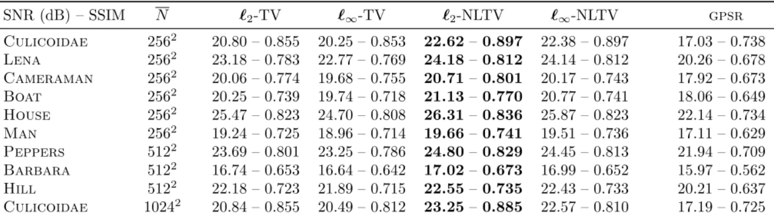
Extensive tests have been carried out on several standard images of different sizes. The SNR and SSIM [91] results obtained by using the various previously introduced TV-like constraints are collected in Table 1. In addition, a comparison is performed between our method and the Gradient Projection for Sparse Reconstruction (GPSR) method [60], which also relies on a variational approach. The constraint bound for both methods was hand-tuned in order to achieve the best SNR values. The best results are highlighted in bold. A visual comparison is made in Figure 1, where two representative images are displayed. These results demonstrate the interest of considering non-local smoothness measures. Non-Local TV with ℓ1,2 -norm indeed proves to be the most effective constraint with gains in SNR and SSIM (up to 1.82 dB and 0.042) with respect to ℓ2-TV, which in turn outperforms GPSR. The better performance of NLTV seems to be related to its ability to better preserve edges and thin structures present in images. In terms of computational time, GPSR is about twice faster thanℓ2-NLTV. Our codes were developed in MATLAB7, the operatorsF andF⊤ being implemented in C using mex files.
In order to complete the analysis, we report in Figure 2 SNR/SSIM comparisons betweenℓ2-NLTV and ℓ2-TV for different blur and noise configurations. These plots show thatℓ2-NLTV provides better results regardless of the degradation conditions.
In the second part of the section, we focus on the convergence speed of epigraph and direct methods. All the results refer to theculicoidae image cropped at 256×256 (N = 2562), since a similar behaviour was
observed for other images. The stopping criterion is set to: kx[i+1]−x[i]k ≤ 10−4kx[i]k. For theℓ 1,p-ball
projectors needed by the direct method, we used the software publicly available on-line [84, 78].
Table 1: SNRdB and SSIM results of our method and GPSR (noise parameters: blur = 3×3, σ = 10, decimation = 60%) SNR (dB) – SSIM N ℓ2-TV ℓ∞-TV ℓ2-NLTV ℓ∞-NLTV gpsr Culicoidae 2562 20.80 – 0.855 20.25 – 0.853 22.62– 0.897 22.38 – 0.897 17.03 – 0.738 Lena 2562 23.18 – 0.783 22.77 – 0.769 24.18– 0.812 24.14 – 0.812 20.26 – 0.678 Cameraman 2562 20.06 – 0.774 19.68 – 0.755 20.71– 0.801 20.17 – 0.743 17.92 – 0.673 Boat 2562 20.25 – 0.739 19.74 – 0.718 21.13– 0.770 20.77 – 0.741 18.06 – 0.649 House 2562 25.47 – 0.823 24.70 – 0.808 26.31– 0.836 25.87 – 0.823 22.14 – 0.734 Man 2562 19.24 – 0.725 18.96 – 0.714 19.66– 0.741 19.51 – 0.736 17.11 – 0.629 Peppers 5122 23.69 – 0.801 23.25 – 0.786 24.80– 0.829 24.45 – 0.813 21.94 – 0.709 Barbara 5122 16.74 – 0.653 16.64 – 0.642 17.02– 0.673 16.99 – 0.652 15.97 – 0.562 Hill 5122 22.18 – 0.723 21.89 – 0.715 22.55– 0.735 22.43 – 0.733 20.21 – 0.637 Culicoidae 10242 20.84 – 0.855 20.49 – 0.812 23.25– 0.885 22.57 – 0.810 17.19 – 0.725
(a) Culicoidae. (b) Degraded. (c) Zoom. (d) GPSR, SNR: 17.03 dB.
(e) Lena. (f) Degraded. (g) Zoom. (h) GPSR, SNR: 20.26 dB. (i)ℓ2-TV, SNR: 20.80 dB. (j)ℓ∞-TV, SNR: 20.25 dB. (k)ℓ2-NLTV, SNR:22.62 dB. (l)ℓ∞-NLTV, SNR: 22.38 dB. (m)ℓ2-TV, SNR: 23.18 dB. (n)ℓ∞-TV, SNR: 22.77 dB. (o)ℓ2-NLTV, SNR:24.18 dB. (p)ℓ∞-NLTV, SNR: 24.14 dB.
Figure 1: Image restoration examples (noise parameters: blur = 3×3,σ= 10, decimation = 60%)
12 34 32 15 16 34 33 37 35 (a) SNR comparison (3 × 3 blur). 12 34 32 15 16 34 33 37 35 (b) SNR comparison (5 × 5 blur). 123 124 125 123 124 125 (c) SSIM comparison (3 ×3 blur). 123 124 125 123 124 125 (d) SSIM comparison (5 ×5 blur).
Figure 2: SNR and SSIM values forℓ2-NLTV (vertical axes) andℓ2-TV (horizontal axes), for theculicoidae image. The plots show the results obtained for σ ∈ {5,10, . . . ,50}, where lower SNR or SSIM values correspond to higherσvalues. No decimation is applied in this experiment.
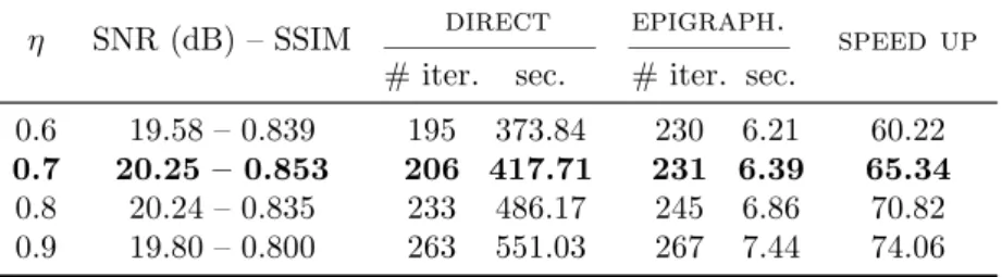
• Total Variation– Tables 2 and 3 report a comparison between the direct and epigraphical methods for different values ofηand forℓ2-TV andℓ∞-TV, respectively. For more readability, these are expressed as a multiplicative factor of the ℓp-TV-semi-norm of the original image. It can be noticed that the parameterη influences both the quality of the results and the convergence speed. For the ℓ1,2-norm, the epigraphical method is 3.5 faster than the direct one. For theℓ1,∞-norm, it is 65 times faster. Figs. 3-a and 3-b show the relative errorkx[i]−x[∞]k/kx[∞]kas a function of the computational time,
wherex[∞]denotes the solution computed after a large number of iterations (typically, 5000 iterations). The dashed line presents the results for the direct method while the solid line refers to the epigraphical one. These plots show that the epigraphical approach is faster despite it requires more iterations in order to converge. This can be explained by the computational cost of the subiterations required by the direct projections onto theℓ1,p-ball.
Table 2: Results for theℓ2-TV constraint and different values ofη
η SNR (dB) – SSIM direct epigraph. speed up # iter. sec. # iter. sec.
0.6 19.70 – 0.839 116 5.74 146 2.23 2.58 0.7 20.62 – 0.862 132 7.14 151 2.29 3.11
0.8 20.80 – 0.855 160 9.17 171 2.59 3.54
0.9 20.45 – 0.826 195 11.95 196 2.98 4.01
Table 3: Results for the ℓ∞-TV constraint and different values ofη
η SNR (dB) – SSIM direct epigraph. speed up # iter. sec. # iter. sec.
0.6 19.58 – 0.839 195 373.84 230 6.21 60.22
0.7 20.25 – 0.853 206 417.71 231 6.39 65.34
0.8 20.24 – 0.835 233 486.17 245 6.86 70.82 0.9 19.80 – 0.800 263 551.03 267 7.44 74.06
• ℓ2-Non-Local Total Variation – Table 4 reports the results for ℓ2-NLTV. Different combinations of neighbourhood size Q and bound value η are considered. To set the weights, the first TV estimate is computed with η = 0.8. The best SNR improvement (1.82 dB over ℓ2-TV) is observed when a relatively small neighbourhood is used (Q= 11). This behaviour was already observed in [90]. It may be related to the bias-variance trade-off commonly encountered in Non-Local filters [92, 93].
In Figure 3-c, a plot similar to those in Figs. 3-a and 3-b show the convergence profile. The epigraphical method requires about the same number of iterations as the direct one in order to converge. This results in a time reduction (1.8 times), as a single iteration of the epigraphical method is faster than one iteration of the direct method.
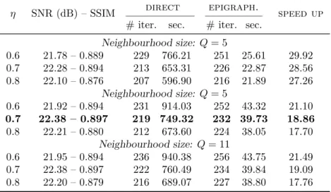
• ℓ∞-Non-Local Total Variation– Table 5 and Figure 3-d show the results obtained with theℓ∞-NLTV constraint. Note thatℓ∞-NLTV requires more iterations thanℓ2-NLTV in order to converge. In what concerns the convergence speed, the epigraphical method is 19 times faster.
Table 4: Results for theℓ2-NLTV constraint and some values ofη andQ
η SNR (dB) – SSIM direct epigraph. speed up # iter. sec. # iter. sec.
Neighbourhood size: Q= 3 0.7 22.26 – 0.895 70 5.82 77 3.07 1.90 0.8 22.41 – 0.893 72 6.39 75 3.00 2.13 0.9 22.06 – 0.875 88 7.97 89 3.58 2.23 Neighbourhood size: Q= 5 0.7 22.44 – 0.900 70 7.13 74 4.37 1.63 0.8 22.58 – 0.898 72 7.85 75 4.44 1.77 0.9 22.25 – 0.880 87 9.71 88 5.24 1.85 Neighbourhood size: Q= 11 0.7 22.50 – 0.901 72 7.52 76 4.51 1.67 0.8 22.61 – 0.897 75 8.21 78 4.64 1.77 0.9 22.27 – 0.879 89 9.83 91 5.41 1.82
Table 5: Results for theℓ∞-NLTV constraint and some values ofηandQ η SNR (dB) – SSIM direct epigraph. speed up
# iter. sec. # iter. sec.
Neighbourhood size: Q= 5 0.6 21.78 – 0.889 229 766.21 251 25.61 29.92 0.7 22.28 – 0.894 213 653.31 226 22.87 28.56 0.8 22.10 – 0.876 207 596.90 216 21.89 27.26 Neighbourhood size: Q= 5 0.6 21.92 – 0.894 231 914.03 252 43.32 21.10 0.7 22.38 – 0.897 219 749.32 232 39.73 18.86 0.8 22.21 – 0.880 212 673.60 224 38.05 17.70 Neighbourhood size: Q= 11 0.6 21.95 – 0.894 236 940.38 256 43.75 21.49 0.7 22.38 – 0.897 222 760.49 234 39.84 19.09 0.8 22.20 – 0.879 216 689.07 227 38.80 17.76
5
Conclusions
We have proposed a new epigraphical technique to solve constrained convex optimization problems with the help of proximal algorithms. In this paper (Part I), our attention has been turned to block-sparsity constraints based on weightedℓ1,p-norms withp∈ {2,+∞}. The obtained results demonstrate the better performance of non-local measures in terms of image quality. Our results also show that the ℓ1,2-norm has to be preferred over the ℓ1,∞-norm for image recovery problems. However, it would be interesting to consider alternative applications ofℓ1,∞-norms such as regression problems [94, 95]. Furthermore, the experimental part indicates that the epigraphical method converges faster than the approach based on the direct computation of the projections via standard iterative solutions. Full implementations in C of the proposed algorithms and parallelization of our codes should even allow us to accelerate them [96]. Note that, although the considered application involves two constraint sets, the proposed approach can handle an arbitrary number of convex constraints. In a companion paper (Part II), we will show that the epigraphical approach can also be used to develop approximation methods for dealing with more general convex constraints.
1
2
3
4
56
726
786
716
756
(a)ℓ2-TV.122
322
422
522
642
632
612
(b)ℓ∞-TV.1
2
3
4
526
578
576
(c)ℓ2-NLTV.1
22
3
22
4
22
53
6
532
576
572
516
(d)ℓ∞-NLTV.Figure 3: Comparison between epigraphical method (solid line) and direct method (dashed line): kx[ki]x−[∞x[]∞k]k in dB vs time
A
Proof of the Proposition 2.4
For every (y, ζ)∈ H ×R, let (p, θ) =Pepiϕ(y, ζ). If ϕ(y)≤ζ, then p=y andθ =ζ = max{ϕ(p), ζ}. In addition, (∀u∈ H) 0 = 1 2kp−yk 2+1 2 max{ϕ(p)−ζ,0} 2 ≤ 12ku−yk2+1 2 max{ϕ(u)−ζ,0} 2 , (43)
which shows that (12) holds. Let us now consider the case when ϕ(y) > ζ. From the definition of the projection, we get
(p, θ) = argmin
(u,ξ)∈epiϕk
u−yk2+ (ξ
−ζ)2. (44)
From the Karush-Kuhn-Tucker theorem [97, Theorem 5.2],8there exists α∈[0,+∞[ such that
(p, θ) = argmin (u,ξ)∈H×R 1 2ku−yk 2+1 2(ξ−ζ) 2+α(ϕ(u) −ξ) (45)
where the Lagrange multiplierαis such that
α(ϕ(p)−θ) = 0. (46) Since the valueα= 0 is not allowable (since it would lead top=y andθ=ζ), it can be deduced from the above equality thatϕ(p) =θ. In addition, differentiating the Lagrange functional in (45) w.r.t. ξyields
ϕ(p) =θ=ζ+α≥ζ. (47)
8By consideringu
Hence, (p, θ) given by (44) is such that p= argmin u∈H ϕ(u)≥ζ ku−yk2+ (ϕ(u)−ζ)2 (48) θ=ϕ(p) = max{ϕ(p), ζ}. (49) Furthermore, asϕ(y)> ζ, we have inf u∈H ϕ(u)≤ζ ku−yk2=kPlev≤ζϕ(y)−yk 2= inf u∈H ϕ(u)=ζ ku−yk2 (50)
where we have used the fact that Plev≤ζϕ(y) belongs to the boundary of lev≤ζϕ which is equal to
u∈ H ϕ(u) =ζ since ϕ is lower-semicontinuous and domϕ is open [73, Corollary 8.38]. We have then inf u∈H ϕ(u)≤ζ ku−yk2= inf u∈H ϕ(u)=ζ ku−yk2 ≥ inf u∈H ϕ(u)≥ζ ku−yk2+ (ϕ(u)−ζ)2. (51)
Altogether, (48) and (51) lead to
p= argmin u∈H 1 2ku−yk 2+1 2 max{ϕ(u)−ζ,0} 2 (52)
which is equivalent to (12) since 12 max{ϕ−ζ,0}2∈Γ0(H).
B
Proof of the Proposition 2.5
Since (max{ϕ−ζ,0})2 is an even function, prox12(max{ϕ−ζ,0})2 is an odd function [23, Remark 4.1(ii)]. In the following, we thus focus on the case wheny∈]0,+∞[.
Ifζ ∈]− ∞,0], then (max{ϕ−ζ,0})2= (ϕ−ζ)2. Whenβ = 1, (max{ϕ−ζ,0})2 =τ2(·)2−2τ ζ| · |+ζ2
and, from Example 2.3, it can be deduced that
prox1 2(max{ϕ−ζ,0})2(y) = prox− τ ζ 1+τ2|·| y 1 +τ2 = 1 1 +τ2max{y+τ ζ,0}. (53)
Whenβ >1, (ϕ−ζ)2 is differentiable and, according to (8),p= prox1
2(max{ϕ−ζ,0})2(y) is uniquely defined as
p−y+βτ pβ−1(τ pβ−ζ) = 0 (54) where, according to [98, Corollary 2.5],p≥0. This allows us to deduce thatp=χ0.
Let us now focus on the case whenζ∈]0,+∞[. Ify∈]0,(ζ/τ)1/β[, it can be deduced from [98, Corollary 2.5], that p= prox1
2(max{ϕ−ζ,0})2(y)∈[0,(ζ/τ)
1/β[. Since (
∀v ∈[0,(ζ/τ)1/β[) max{ϕ(v)−ζ,0}= 0, (8) yields
p=y. On the other hand ify >(ζ/τ)1/β, as the proximity operator of a function fromRtoRis continuous
and increasing [98, Proposition 2.4],p= prox1
2(max{ϕ−ζ,0})2(y)≥prox12(max{ϕ−ζ,0})2 (ζ/τ)
1/β= (ζ/τ)1/β.
Since (max{ϕ−ζ,0})2is differentiable in this case, and (
∀v≥(ζ/τ)1/β) (max
{ϕ(v)−ζ,0})2= (τ vβ
−ζ)2,
(8) allows us to deduce that pis the unique value in [(ζ/τ)1/β,+
∞[ satisfying (54). It can be concluded that, whenζ∈]0,+∞[, (16) holds.
C
Proof of the Proposition 2.6
Let us notice that 12(max{τ d
β
C−ζ,0})2 = ψ◦dC where ψ = 12(max{τ| · |β −ζ,0})2. According to [25,
Proposition 2.7], for everyy∈ H,
proxψ◦dC(y) = y, ify∈C, PC(y), ify6∈C anddC(y)≤max∂ψ(0), αy+ (1−α)PC(y), ifdC(y)>max∂ψ(0) (55) whereα= proxψ dC(y) dC(y) . In addition, we have ∂ψ(0) = ( [τ ζ,−τ ζ], ifζ <0 andβ = 1, {0}, otherwise, (56)
and, according to Proposition 2.5, whenζ < 0,β = 1 anddC(y)≤ −τ ζ, proxψ dC(y)
= 0. These show that (55) reduces to (17).
D
Proof of the Corollary 2.7
As we have ϕ = τ dC where C = {z}, the result follows from Proposition 2.6 and the expression of
prox1
2(max{τ|·|−ζ,0})2 in Proposition 2.5.
E
Proof of the Proposition 2.8
The function ϕ belongs to Γ0(R) since for every m ∈ {1, . . . , M}, v 7→ max{τ(m)(ν(m)−v),0} is finite
convex and (·)2 is finite convex and increasing on [0,+∞[. In addition, ϕis differentiable and it is such
that, for everyv∈Rand everyk∈ {1, . . . , M+ 1},
ν(k−1)< v ≤ν(k) ⇒ ϕ(v) = 1 2 kX−1 m=1 (τ−(m))2v −ν(m)2+1 2 M X m=k (τ+(m))2 v−ν(m)2. (57)
For every y ∈ R, as p = prox
ϕ(y) is characterized by (8), there exists m ∈ {1, . . . , M+ 1} such that ν(m−1)< p≤ν(m) and y−p= mX−1 m=1 (τ−(m))2(p−ν(m)) + M X m=m (τ+(m))2(p−ν(m)). (58)
This yields (21), and we have : (22)⇔ν(m−1)< p≤ν(m). The uniqueness ofm∈ {1, . . . , M+ 1}satisfying
F
Proof of the Proposition 3.2
For every (y(ℓ), ζ(ℓ))∈RM(ℓ)×R, in order to determinePepih(ℓ)(y(ℓ), ζ(ℓ)) we have to find min θ(ℓ)∈[0,+∞[ (θ(ℓ)−ζ(ℓ))2+ min |p(ℓ,1)|≤τ(ℓ,1)θ(ℓ) .. . |p(ℓ,M (ℓ)) |≤τ(ℓ,M(ℓ))θ(ℓ) kp(ℓ)−y(ℓ)k2 . (59)
For everyθ(ℓ)∈[0,+∞[, the inner minimization is achieved when, for everyj ∈ {1, . . . , M(ℓ)},p(ℓ,m)is the
projection ofy(ℓ,m)onto [−τ(ℓ,m)θ(ℓ), τ(ℓ,m)θ(ℓ)], which is given by (34). Then, the problem reduces to
minimize θ(ℓ)∈R (θ(ℓ)−ζ(ℓ))2+ M(ℓ) X m=1 (max{|y(ℓ,m)| −τ(ℓ,m)θ(ℓ),0})2+ι[0,+∞[(θ(ℓ)) (60)
which is also equivalent to calculate proxϕ+ι[0,+∞[(ζ
(ℓ)), where ϕis such that
(∀v∈R) ϕ(v) =1 2
MX(ℓ) m=1
(max{τ(ℓ,m)(ν(ℓ,m)−v),0})2. (61)
By using now the fact that proxϕ+ι[0,+∞[ =P[0,+∞[◦proxϕ([24, Proposition 12]) and by invoking Proposition 2.8, the expression of the optimal solution in (35) follows.
References
[1] L. Chaari, J.-C. Pesquet, A. Benazza-Benyahia, and Ph. Ciuciu, “A wavelet-based regularized re-construction algorithm for SENSE parallel MRI with applications to neuroimaging,” Medical Image Analysis, vol. 15, no. 2, pp. 185–201, Apr. 2011.
[2] M. Guerquin-Kern, M. H¨aberlin, K.P. Pruessmann, and M. Unser, “A fast wavelet-based reconstruction method for magnetic resonance imaging,” IEEE Trans. Med. Imag., vol. 30, no. 9, pp. 1649–1660, Sep. 2011.
[3] G. Facciolo, A. Almansa, J.-F. Aujol, and V. Caselles, “Irregular to regular sampling, denoising, and deconvolution,” Multiscale Model. and Simul., vol. 7, no. 4, pp. 1574–1608, Avr. 2009.
[4] N. Hajlaoui, C. Chaux, G. Perrin, F. Falzon, and A. Benazza-Benyahia, “Satellite image restoration in the context of a spatially varying point spread function,” J. Opt. Soc. Am., vol. 27, no. 6, pp. 1473–1481, 2010.
[5] F.-X. Dup´e, M. J. Fadili, and J.-L. Starck, “A proximal iteration for deconvolving Poisson noisy images using sparse representations,” IEEE Trans. Image Process., vol. 18, no. 2, pp. 310–321, Feb. 2009. [6] A. Jezierska, E. Chouzenoux, J.-C. Pesquet, and H. Talbot, “A primal-dual proximal splitting approach
for restoring data corrupted with Poisson-Gaussian noise,” inProc. Int. Conf. Acoust., Speech Signal Process., Kyoto, Japan, Mar., 25-30 2012, 4p.
[7] B. Vandeghinste, B. Goossens, J. De Beenhouwer, A. Pizurica, W. Philips, S. Vandenberghe, and S. Staelens, “Split-Bregman-based sparse view CT reconstruction,” in International Meeting on Fully Three-Dimensional Image Reconstruction in Radiology and Nuclear Medicine, Potsdam, Germany, Jul. 11-15 2011.
[8] N. Pustelnik, C. Chaux, J.-C. Pesquet, and C. Comtat, “Parallel algorithm and hybrid regularization for dynamic PET reconstruction,” inIEEE Med. Imag. Conf., Knoxville, Tennessee, Oct. 30 - Nov. 6 2010.
[9] S. Anthoine, J.-F. Aujol, Y. Boursier, and C. M´elot, “Some proximal methods for CBCT and PET tomography,” in Mathematical imaging in interaction with biomedicine, Edinburgh, Scotland, Sept., 05-09 2011.
[10] J.-F. Aujol, G. Aubert, L. Blanc-F´eraud, and A. Chambolle, “Image decomposition into a bounded variation component and an oscillating component,” J. Math. Imag. Vis., vol. 22, pp. 71–88, Jan. 2005. [11] J.-F. Aujol, G. Gilboa, T. Chan, and S. Osher, “Structure-texture image decomposition - modeling,
algorithms, and parameter selection,” Int. J. Comp. Vis., vol. 67, no. 1, pp. 111–136, Apr. 2006. [12] L. M. Brice˜no-Arias, P. L. Combettes, J.-C. Pesquet, and N. Pustelnik, “Proximal algorithms for
multicomponent image recovery problems,” J. Math. Imag. Vis., vol. 41, no. 1, pp. 3–22, Sep. 2011. [13] F. Bach, R. Jenatton, J. Mairal, and G. Obozinski, “Optimization with sparsity-inducing penalties,”
Foundations and Trends in Machine Learning, vol. 4, no. 1, pp. 1–106, 2012.
[14] S. Theodoridis, K. Slavakis, and I. Yamada, “Adaptive learning in a world of projections,”IEEE Signal Process. Mag., vol. 28, no. 1, pp. 97–123, Jan. 2011.
[15] C. Chaux, M. El Gheche, J. Farah, J.-C. Pesquet, and B. Pesquet-Popescu, “A parallel proximal splitting method for disparity estimation from multicomponent images under illumination variation,”
J. Math. Imag. Vis., 2012, To appear.
[16] M. Kowalski, E. Vincent, and R. Gribonval, “Beyond the narrowband approximation: Wideband convex methods for under-determined reverberant audio source separation,”IEEE Trans. Audio, Speech Language Process., vol. 18, no. 7, pp. 1818–1829, Sept. 2010.
[17] O. D. Akyildiz and I. Bayram, “An analysis prior based decomposition method for audio signals,” in
Proc. Eur. Sig. and Image Proc. Conference, Bucharest, Romania, Aug. 27-31 2012.
[18] P. L. Combettes and J.-C. Pesquet, “Proximal splitting methods in signal processing,” inFixed-Point Algorithms for Inverse Problems in Science and Engineering, H. H. Bauschke, R. S. Burachik, P. L. Combettes, V. Elser, D. R. Luke, and H. Wolkowicz, Eds., pp. 185–212. Springer-Verlag, New York, 2011.
[19] S. Setzer, G. Steidl, and T. Teuber, “Deblurring Poissonian images by split Bregman techniques,” J. Visual Communication and Image Representation, vol. 21, no. 3, pp. 193–199, Apr. 2010.
[20] M. A. T. Figueiredo and J. M. Bioucas-Dias, “Restoration of Poissonian images using alternating direction optimization,” IEEE Trans. Image Process., vol. 19, no. 12, pp. 3133–3145, Dec. 2010. [21] J.-C. Pesquet and N. Pustelnik, “A parallel inertial proximal optimization method,” Pac. J. Optim.,
vol. 8, no. 2, pp. 273–305, Apr. 2012.
[22] P. L. Combettes and V. R. Wajs, “Signal recovery by proximal forward-backward splitting,” Multiscale Model. and Simul., vol. 4, no. 4, pp. 1168–1200, Nov. 2005.
[23] C. Chaux, P. L. Combettes, J.-C. Pesquet, and V. R. Wajs, “A variational formulation for frame-based inverse problems,” Inverse Problems, vol. 23, no. 4, pp. 1495–1518, Jun. 2007.
[24] P. L. Combettes and J.-C. Pesquet, “A Douglas-Rachford splitting approach to nonsmooth convex variational signal recovery,” IEEE J. Selected Topics Signal Process., vol. 1, no. 4, pp. 564–574, Dec.
[25] P. L. Combettes and J.-C. Pesquet, “A proximal decomposition method for solving convex variational inverse problems,” Inverse Problems, vol. 24, no. 6, Dec. 2008.
[26] N. P. Galatsanos and A. K. Katsaggelos, “Methods for choosing the regularization parameter and estimating the noise variance in image restoration and their relation,” IEEE Trans. Image Process., vol. 1, no. 3, pp. 322–336, Jul. 1992.
[27] P. C. Hansen and D. P. O’Leary, “The use of the L-curve in the regularization of discrete ill-posed problems,” SIAM J. Sci. Comput., vol. 14, no. 6, pp. 1487–1503, 1993.
[28] A. Pizurica and W. Philips, “Estimating the probability of the presence of a signal of interest in multiresolution single- and multiband image denoising,” IEEE Trans. Image Process., vol. 15, no. 3, pp. 654–665, Mar. 2006.
[29] S. Ramani, T. Blu, and M. Unser, “Monte-Carlo SURE: A black-box optimization of regularization parameters for general denoising algorithms,” IEEE Trans. Image Process., vol. 17, no. 9, pp. 1540– 1554, Sep. 2008.
[30] L. Chaari, J.-C. Pesquet, J.-Y. Tourneret, P. Ciuciu, and A. Benazza-Benyahia, “A hierarchical bayesian model for frame representation,” IEEE Trans. Signal Process., vol. 58, no. 11, pp. 5560–5571, Nov. 2010.
[31] D. C. Youla and H. Webb, “Image restoration by the method of convex projections. Part I - theory,”
IEEE Trans. Med. Imag., vol. 1, no. 2, pp. 81–94, Oct. 1982.
[32] H. J. Trussell and M. R. Civanlar, “The feasible solution in signal restoration,” IEEE Trans. Acous., Speech Signal Process., vol. 32, no. 2, pp. 201–212, Apr. 1984.
[33] P. L. Combettes, “Inconsistent signal feasibility problems : least-squares solutions in a product space,”
IEEE Trans. Signal Process., vol. 42, no. 11, pp. 2955–2966, Nov. 1994.
[34] K. Kose, V. Cevher, and A. E. Cetin, “Filtered variation method for denoising and sparse signal processing,” inProc. Int. Conf. Acoust., Speech Signal Process., Kyoto, Japan, March, 27-30 2012. [35] T. Teuber, G. Steidl, and R. H. Chan, “Minimization and parameter estimation for seminorm
regu-larization models with I-divergence constraints,” Tech. Rep., Technische Universit¨at Kaiserslautern, 2012.
[36] R. Ciak, B. Shafei, and G. Steidl, “Homogeneous penalizers and constraints in convex image restoration,”
J. Math. Imag. Vis., 2012.
[37] L. Jacques, L. Duval, C. Chaux, and G. Peyr´e, “A panorama on multiscale geometric representations, intertwining spatial, directional and frequency selectivity,” Signal Process., vol. 91, no. 12, pp. 2699– 2730, Dec. 2011.
[38] M. A. T. Figueiredo and R. D. Nowak, “An EM algorithm for wavelet-based image restoration,”IEEE Trans. Image Process., vol. 12, no. 8, pp. 906–916, Aug. 2003.
[39] M. V. Afonso, J. M. Bioucas-Dias, and M. A. T. Figueiredo, “An augmented Lagrangian approach to the constrained optimization formulation of imaging inverse problems,” IEEE Trans. Image Process., vol. 20, no. 3, pp. 681–695, Mar. 2011.
[40] A. Tikhonov, “Tikhonov regularization of incorrectly posed problems,” Soviet Mathematics Doklady, vol. 4, pp. 1624–1627, 1963.
[41] E. Chouzenoux, J. Idier, and S. Moussaoui, “A Majorize-Minimize strategy for subspace optimization applied to image restoration,” IEEE Trans. Image Process., vol. 20, no. 6, pp. 1517–1528, Jun. 2011.
[42] G. Aubert and R. Tahraoui, “Sur la minimisation d’une fonctionnelle non convexe, non diff´erentiable en dimension 1,” Bolletino UMI, vol. 5, no. 17B, 1980.
[43] A. Ben-Tal and M. Teboulle, “A smoothing technique for nondifferentiable optimization problems,”
Lecture Notes in Mathematics, vol. 1405, pp. 1–11, 1989.
[44] J.-B. Hiriart-Urruty and C. Lemar´echal, Convex analysis and minimization algorithms, Part I : Fun-damentals, vol. 305 ofGrundlehren der mathematischen Wissenschaften, Springer-Verlag, Berlin, Hei-delberg, N.Y., 2nd edition, 1996.
[45] P. Tseng, “Convergence of a block coordinate descent method for nondifferentiable minimization,”
Journal of Opt. Theory and Applications, vol. 109, no. 3, pp. 475–494, Jun. 2001. [46] S. J. Wright, Primal-dual interior-point methods, SIAM, Philadelphia, PA, 1997.
[47] L. M. Bregman, “The method of successive projection for finding a common point of convex sets,”
Soviet Math. Dokl., vol. 6, pp. 688–692, 1965.
[48] L. G. Gurin, B. T. Polyak, and E. V. Raik, “Projection methods for finding a common point of convex sets,” Zh. Vychisl. Mat. Mat. Fiz., vol. 7, no. 6, pp. 1211–1228, 1967.
[49] P. L. Combettes, “The foundations of set theoretic estimation,” Proceedings of the IEEE, vol. 81, no. 2, pp. 182–208, Feb. 1993.
[50] P. L. Combettes, “Convex set theoretic image recovery by extrapolated iterations of parallel subgradient projections,” IEEE Trans. Image Process., vol. 6, no. 4, pp. 492–506, Apr. 1997.
[51] Y. Censor, W. Chen, P. L. Combettes, R. Davidi, and G. T. Herman, “On the effectiveness of projection methods for convex feasibility problems with linear inequality constraints,” Comput. Optim. Appl., vol. 51, no. 3, pp. 1065–1088, 2012.
[52] B. T. Polyak, “Minimization of unsmooth functionals,” USSR Computational Mathematics and Math-ematical Physics, vol. 9, no. 3, pp. 14–29, 1969.
[53] N. Z. Shor, Minimization Methods for Non-differentiable Functions, Springer-Verlag, New York, 1985. [54] P. L. Combettes, “A block-iterative surrogate constraint splitting method for quadratic signal recovery,”
IEEE Trans. Signal Process., vol. 51, no. 7, pp. 1771–1782, Jul. 2003.
[55] K. Slavakis, I. Yamada, and N. Ogura, “The adaptive projected subgradient method over the fixed point set of strongly attracting nonexpansive mappings,” Numerical Functional Analysis and Optimization, vol. 27, no. 7-8, pp. 905–930, Nov. 2006.
[56] P. Bouboulis, K. Slavakis, and S. Theodoridis, “Adaptive learning in complex reproducing kernel Hilbert spaces employing Wirtinger’s subgradients,” IEEE Trans Neural Networks, vol. 23, no. 3, pp. 425–438, Mar. 2012.
[57] J. J. Moreau, “Proximit´e et dualit´e dans un espace hilbertien,” Bull. Soc. Math. France, vol. 93, pp. 273–299, 1965.
[58] D. L. Donoho, “De-noising by soft-thresholding,” IEEE Trans. Inform. Theory, vol. 41, no. 3, pp. 613–627, May 1995.
[59] I. Daubechies, M. Defrise, and C. De Mol, “An iterative thresholding algorithm for linear inverse problems with a sparsity constraint,” Comm. Pure Applied Math., vol. 57, no. 11, pp. 1413–1457, Nov. 2004.
![Figure 3: Comparison between epigraphical method (solid line) and direct method (dashed line): kx [i] kx −x [∞] [∞] k k](https://thumb-us.123doks.com/thumbv2/123dok_us/11107459.2998483/17.892.106.803.168.497/figure-comparison-epigraphical-method-solid-direct-method-dashed.webp)
