Fast Gibbs sampling for high-dimensional Bayesian inversion

(1)

This content has been downloaded from IOPscience. Please scroll down to see the full text.

Download details:

IP Address: 128.41.35.12

This content was downloaded on 07/11/2016 at 15:41

Please note that terms and conditions apply.

Fast Gibbs sampling for high-dimensional Bayesian inversion

View the table of contents for this issue, or go to the journal homepage for more 2016 Inverse Problems 32 115019

(2)

Fast Gibbs sampling for high-dimensional

Bayesian inversion

Felix Lucka

Centre for Medical Image Computing, University College London, WC1E 6BT London, UK

E-mail:[email protected]

Received 27 February 2016, revised 28 June 2016 Accepted for publication 7 September 2016 Published 7 October 2016

Abstract

Solving ill-posed inverse problems by Bayesian inference has recently attracted considerable attention. Compared to deterministic approaches, the probabilistic representation of the solution by the posterior distribution can be exploited to explore and quantify its uncertainties. In applications where the inverse solution is subject to further analysis procedures can be a signiﬁcant advantage. Alongside theoretical progress, various new computational techniques allow us to sample very high dimensional posterior distributions: in (Lucka 2012 Inverse Problems 28

125012), and a Markov chain Monte Carlo posterior sampler was developed for linear inverse problems withℓ1-type priors. In this article, we extend this single component(SC)Gibbs-type sampler to a wide range of priors used in Bayesian inversion, such as generalℓ_pqpriors with additional hard constraints. In addition, a fast computation of the conditional, SC densities in an explicit, parameterized form, a fast, robust and exact sampling from these one-dimensional densities is key to obtain an efficient algorithm. We demonstrate that a generalization of slice sam-pling can utilize their specific structure for this task and illustrate the performance of the resulting slice-within-Gibbs samplers by different computed examples. These new samplers allow us to perform sample-based Bayesian inference in high-dimensional scenarios with certain priors for thefirst time, including the inversion of computed tomography data with the popular isotropic total variation prior. Keywords: Bayesian inversion, MCMC, Gibbs sampler, slice sampling, computed tomography, total variation prior

(Someﬁgures may appear in colour only in the online journal)

Inverse Problems32(2016)115019(23pp) doi:10.1088/0266-5611/32/11/115019

Original content from this work may be used under the terms of theCreative Commons Attribution 3.0 licence. Any further distribution of this work must

maintain attribution to the author₍s₎and the title of the work, journal citation and DOI.

(3)

1. Introduction 1.1. Bayesian inversion

We consider the task of inferring information about an unknown quantity from indirect, noisy measurements and assume that a reasonable mathematical model is given by a linear, ill-posed operator equation including additive noise terms. The following discrete forward model is used to carry out the computational inference:

e

= +

f A u . ( )1

Here, fÎm_{represents the measured data,}_u_În _{a suitable discretization of the unknown} quantity we wish to reconstruct and AÎm´n _{a corresponding discretization of the} continuous forward operator. We assume that the statistics of the additive noise can be well-approximated by a Gaussian distribution (m,S)and thatfandAare already centered and decorrelated with respect toμandΣ, i.e., f= S-1 2_{( ˜}f -m₎_and_A _{= S}-1 2_A˜_{, where} _f˜_and A˜ denote the original data and forward operator, respectively. This leads toe~(0,Im)and the followinglikelihooddistribution

µ -  -  p_like f u exp 1 f A u , 2 2 2 2

(

)

( ∣ ) ( )

which is a probabilistic model of the measured datafgiven the unknown solutionu. In typical inverse problems, solving (1)foru is ill-posed. As a consequence, the information that(2) contains about u is insufﬁcient to carry out robust inference and we need to amend it by

a prioriinformation, encoded ina priordistributionp_prior( ). Then, the total information onu u

we have afterperforming the measurement is encoded by the conditional distribution of u

givenf, the so-calleda posterioridistribution. It can be computed byBayes’rule: = p u f p f u p u p f . 3 post like prior ( ∣ ) ( ∣ ) ( ) ( ) ( )

Figure 1 illustrates the inference process. Originating from statistical physics, Gibbs distributionsare commonly used prior models:

 l

µ

-p_prior( )u exp( ( ))u . ( )4

The functional( )u measures anenergy ofu. The use of Gibbs priors leads to

 l µ -  -  -p_post u f exp 1 f A u u . 5 2 2 2

(

)

( ∣ ) ( ) ( )

For a general introduction toBayesian inversionwe refer to[20,28,39]and references therein. The recent attention on this particular inversion approach is best reﬂected by the recent special issue of

Inverse Problems[7], which also provides a good overview over current developments and trends. 1.2. Sample-based inference

While the posterior p_post( ∣ )u f represents our complete knowledge about u, Bayesian esti-mationtries to extract the information of interest from it. Classical examples thereof include the maximum a posteriori estimate(MAP)and the and theconditional mean estimate(CM)

 

ò

= Î u argmax p u f , u u f u p u f d ,u 6 u

MAP post CM post

n

ˆ ≔ { ( ∣ )} ˆ ≔ [ ∣ ] ( ∣ ) ( ) which both yield a single point estimate ofu. The details on their properties and relationship can be found in [6]. More sophisticated estimators such asconditional covariance(CCov),

(4)

statistics ofu, or try to quantify the uncertainties ofu, for instance throughcredible region/ intervaland extreme value probabilityestimators.

Bayesian computationrefers to the practical task of computing the above estimators. For most inversion scenarios and prior models, this involves solving high-dimensional optim-ization or integration tasks (see(6)), or even a mix of both. In this article, we are examining techniques that integrate p_post( ∣ )u f byMonte Carlo integration:

ò

g u p u f u»

å

K g u d 1 , 7 i K i post ( ) ( ∣ ) ( ) ( )

where uiare samples of p_post( ∣ )u f generated by asampling algorithm/sampler. Due to the lack of efficient direct samplers that generate i.i.d. samples, Markov chain Monte Carlo (MCMC) samplers need to be employed in most situations. MCMC for high dimensional Bayesian inversion is a very active field of research, see, e.g.,[1,2,4,11,12,16,22,31– 33,36–38]for some examples of recent developments. In[27], an efficient MCMC sampler for Gibbs priors with ℓ1-norm-type energies(ℓ1-priors, seefigure 1(b))was presented:

l

µ -  

p u exp D uT . 8

prior( ) ( 1) ( )

Such energies are commonly used to impose sparsity constraints on the solution of high dimensional image reconstruction problems, a direction of research closely related to the notion of compressed sensing [8, 14, 15]. A detailed discussion of sparsity as a priori

information in Bayesian inversion can be found in [28]. The sampler developed in [27] belongs to the class of single component(SC)Gibbs samplers, which sample p_post( ∣ )u f by subsequently sampling along the conditional, SC densities ppost( ∣u uj -j,f):

Algorithm 1. (SC-Gibbs sampling)

Deﬁne an initial stateu0, a burn-in sizeK0and sample sizeK. Fori=1,¼,K0+K do:

A1.1 Choose a component j(deterministic or random). A1.2 Drawy~ppost( · ∣u-j,f).

A1.3 Setuj+ =y i 1 _{, and} ₌ -+ -u j u i j i 1 . Discard ui ₌ i K 0 0 { } and use ui ₌+₊ i K K K 1 0 0 { } as a sample of p_post( ∣ )u f .

Figure 1.(a)–(b)Illustration of Bayesian inversion with different priors. Depicted are the level sets of likelihood(green, dashed), prior(red, dotted)and resulting posterior distribution (blue, solid). Maximal and expected values of the corresponding distributions are depicted by a star and a bullet, respectively. (c) Example of an MCMC chain generated by an SC Gibbs sampler(blue bullets connected by dashed lines)to sample a bivariate target density(level sets shown as red solid lines).

(5)

We have usedx-j≔ (x1,¼,xj-1,xj+1,¼,xn)Tto denote a vector with all components of

x except forxj. An illustration of Gibbs sampling is given inﬁgure1(c). In [27], this

SC-Gibbs sampler was compared to the popular Metropolis–Hastings (MH) sampler: for the computational scenarios considered and the evaluation performed, it was demonstrated that in contrast to the MH, SC-Gibbs sampling gets more efﬁcient when the level of sparsity or the dimension of the unknowns is increased. Thereby, it became possible to carry out sample-based inference withℓ1priors in challenging inverse problems scenarios withn>106:

• The theoretical predictions about the inﬁnite dimensional limits of total variation (TV) priors posed in[10,24]could be veriﬁed numerically(see[28]).

• Computed tomography (CT) inversion with Besov space priors (see [18, 21]) was examined for simulated and experimental data(see[6,28]).

• The numerical results stimulated the development of new theoretical ideas about the relationship of MAP and CM estimates(see[6,19]).

1.3. Previous limitations

As the sampler developed in[27]relies on a direct sampling of the SC densities, namely the

inverse cumulative distribution method(iCDF), we will call it thedirectℓ1samplerfrom now on. While the directℓ1sampler works well in the applications described above, it suffers from several limitations. To understand them, we recall that an efﬁcient SC-Gibbs sampler needs to:

(SC1) Compute the conditional, SC densities in an explicit, parameterized form in a fast way.

(SC2) Employ a fast, robust and exact sampling scheme for the parameterized form of the SC densities.

In order to best fulfill (SC1) and (SC2), the direct ℓ1 sampler was designed for a very particular setting: firstly, in addition to relying on a linear forward map(1)and a Gaussian noise model(2), it assumes that the operatorDÎn´h_in₍₈₎_{can be diagonalized}₍_synthesis priors): there is a basis matrixVsuch thatD VT _{is a diagonal matrix}_W_Îhń_{. The direct}_ℓ 1 sampler then samples over the coefficients ofu =Vx in this basis:

x µ -  - x -l  x p_post f exp 1 f AV W . 9 2 2 2 1

(

)

( ∣ ) ( )

This excludes the use offramesordictionariesforD. Secondly, it only works for theℓ1norm as a prior energy: a straight-forward extension of iCDF to examine more generalℓ_pq-prior of the form p u µexp -lD uT 

p q

prior( ) ( )is not possible. This excludes the interesting cases of

= <

q p p, 1, which leads to a non-convex energy but also p=1, q>1, which was examined in[10]. Finally, a lot of interesting priors such as the popular isotropic TV prior in 2D/3D or related,bloc/structured sparsitypriors have a more involved structure than(8)and cannot be treated with iCDF in an efﬁcient and robust way as well. In all the above cases, including additionalhard constraints,uÎ, where is thefeasible setof solutions is often advantageous: ⎧ ⎨ ⎩   µ  = Î p u p u u p u ifu , 0 otherwise. 10

prior( ) ˜prior( ) · ( ) prior ˜ ( )

( ) While such constraints have proven to be very useful as a priori knowledge [3,40], their inclusion into the directℓ1sampler in a numerically stable way is cumbersome.

(6)

1.4. Contributions and structure

For most of the limitations discussed above, the main problem is not to fulfill(SC1), but to fulfill(SC2)by using a direct sampler such as iCDF for the parameterized SC densities in step A1.2. In this article, we sample from them by using a generalization ofslice samplingthat utilizes their specific structure instead and demonstrate the effectiveness of this replacement in different computed examples. This allows us to perform sample-based Bayesian inference in high-dimensional scenarios with the priors described above for thefirst time.

The paper is structured as follows: in section 2, weﬁrst derive the SC densities for the priors discussed above. Then, we introduce the basic and generalized slice sampler and discuss how to integrate it into the SC Gibbs sampler for Bayesian inversion. Section 3 contains computed examples and section4closes with a discussion. Several technical details are covered in section appendixA.

2. Sampling methods

For general and comprehensive introductions to MCMC sampling methods, we refer to[26,34].

2.1. SC posteroir densities

In this section, we briefly derive the SC posterior densities for the examined prior models in a simple, parameterized way, see(SC1). Wefirst discuss the case where a basis{v1,¼,vn}helps to representu= åx_{l l}v ≕ Vx such that ppost( ∣x xj _-j,f)can be described using as few para-meters as possible. Once such a basis is found, the part of ppost( ∣x xj _-j,f)coming from the likelihood is easy to derive: we defineY≔ AV andj( ) ≔j f- Y_{- -}jx j. Then, wefind that

x x x x j x x j x - = - = - Y = - Y + Y = - Y µx Y + Y -            f Au f AV f f j i ax bx, 11 j j j j j j j j _j j T j 1 2 2 2 1 2 2 2 1 2 2 2 1 2 2 2 1 2 2 2 1 2 2 2 2 2 ( ) ( ) ( ) ≕ ( ) where we introducedx ≔x_j,a  Yj 1 2 2 2 ≔ , andb ≔YTjj( )j = Y - Y YTjf ( Tj _-j)x_-jto ease the notation for the following sections. Note that while a and YTjf can be precomputed,

x

Y YTj -j -j

( ) relies on the current state of theξ-chain and has to be computed in every step of the sampler. Especially for complicated forward operators in high-dimensional scenarios, this operation is the computational bottleneck of SC Gibbs samplers. Therefore, a careful, scenario-dependent implementation is important to obtain a fast sampler.

Now we proceed to determineVand the part of ppost( ∣x xj _-j,f)coming from the prior. The energies of theℓ_pq priors can be written as

⎛ ⎝ ⎜ ⎞ ⎠ ⎟ ⎛ ⎝ ⎜⎜ ⎞ ⎠ ⎟⎟  u =

å

D u =

å å

D v x . 12 k h k T p q p k h l k T l l p q_p ( ) ∣ ∣ ( ) ( )

To obtain simple conditional densities for allx_j, we thus have to chooseVsuch that ¹

D v u k u

max , where card 0 , 13

l T

l0 0 k

∣ ∣ ∣ ∣ ≔ ({ ∣ }) ( )

is as small as possible. Weﬁrst consider the special but important case ofDT Îh´n_having full rank andhn. This includes the case where the columnsDare elements of a basis, and thereby, the class of Besov priors, see [6, 13, 18, 21, 23] and the TV prior in 1D with

(7)

Neumann boundary conditions, which we will use in the computational studies. Due to the full rank, we can choose v1,¼,vh such thatD vT l=el forl=1,¼,h, andvh+1,¼,vn such that D vT =0

l for l =h +1,¼,n (for D being a basis, we have V=D). With this transformation, (12)simpliﬁes to:

⎛ ⎝ ⎜ ⎞ ⎠ ⎟ ⎛ ⎝ ⎜⎜ ⎞ ⎠ ⎟⎟  x µ

å

x = x +

å

x ¹ . 14 l h lp jp l j h lp q p q p ( ) ∣ ∣ ∣ ∣ ∣ ∣ ( )

Deﬁning x ≔ x_jas above, we can write the conditional SC posterior density as:



å

l x µ - + - + ¹  p x exp ax bx c xp d q p , c , d , 15 j h l j h l p 2 ( ) ( (∣ ∣ ) ) ≔ { } ≔ ∣ ∣ ( ) which simpliﬁes to  l µ - + -  p x exp ax bx c xp , c , 16 j h 2 ( ) ( ∣ ∣ ) ≔ { } ( )

forℓ_pp priors. In the case whereDcannot be diagonalized, an explicit form is given by

⎛ ⎝ ⎜ ⎜⎜ ⎛ ⎝ ⎜⎜ ⎞ ⎠ ⎟⎟ ⎞ ⎠ ⎟ ⎟⎟

å

µ - + - -Î p x exp ax bx c d x e , 17 k D v k kp q p 2 supp T j ( ) ∣ ∣ ( ) ( )  l _{- -}x c d D v e D V where ≔ {j h}, k ≔ ( T j k) , k ≔ ( T j j k) . (18)

Various generalizations of the standardℓ_pqpriors withD uT  p

q_{-type energies}_ﬁ_{rst compute the} ℓ2-norm of alocal featureofu, e.g., of its gradient, and then measure theglobalℓpqenergy of these local ℓ2 norms In this article, we will only discuss one prominent example thereof, which is given by the isotropic TV prior in 2D: if we assume that u represents an N×N

discrete image, we can index the components of u asu(k l,) with k=1,¼,N,l=1,¼,N,

=

n N2_{. We can then use forward differences in both spatial directions to de}_ﬁ_ne

i u =

å

u + -u + u + -u , 19 k l n k l k l k l k l TV , 1, , 2 , 1 , 2 ( ) ( ) ( ) ( ) ( ) ( ) ( ) ( ) ( )

with appropriate additional boundary conditions. The local nature of theiTV( )u allows us to derive a simple parameterization of the SC densities in the pixel basis V=In. Every

x_j=u(k l,)only appears in three terms of the energy:

 µ - + -+ - + -+ - + -- + + - - + -+ - - -u u u u u u u u u u u u u u . 20 i k l k l k l k l k l k l k l k l k l k l k l k l k l k l k l TV , , , 1, , 2 , 1 , 2 , 1, 2 1, 1 1, 2 1, 1 , 1 2 , , 1 2 ( ∣ ) ( ) ( ) ( ) ( ) ( ) ( ) ( ) ( ) ( ) ( ) ( ) ( ) ( ) ( ) ( ) ( ) ( ) ( ) ( ) ( ) ( ) ( )

Therefore, we can write the conditional SC posterior as

⎛ ⎝ ⎜ ⎞ ⎠ ⎟

å

µ - + - - + = p x exp ax bx c d x e g , 21 k k k k 2 1 3 2 ( ) ( ) ( )

with appropriately computed parametersdkÎ{0, 1, 2},ek,gk0.

The difﬁculty of incorporating additional hard constraints(10)depends on the shape of the feasible setand the transformationVapplied. In the following, we assume that they lead to a feasible(semi-)ﬁnite interval[lb ub, ]to which the continuous densities computed above

(8)

can be restricted to. In the case ofbeing convex, such an interval always exists and there are computationally efﬁcient ways to compute it.

2.2. MCMC-within-Gibbs sampling

The directℓ1sampler is sampling(16)withp=1 by the iCDF method using an explicit form of the inverse CDF. For p q, ¹1or(21)this is not possible and one would need to integrate the CDF numerically to use the iCDF method as a SC density sampler. However, already for

p=1, a major technical difficulty was to develop a numerical implementation that worked for all possible combinations (a b c, , ): the first implementations broke down when the dimension n of the problem was increased and the ill-posedness became more severe. The reason was that combinations of(a b c, , )corresponding to extremely degenerate SC densities appeared more frequently forn  ¥and in general, the variability of SC densities grows. This trend will be an even more severe problem when one cannotfind an explicit form of the inverse CDF and needs so resort to numerical integration. But also replacing the iCDF method by a univariate MCMC sampler(MCMC-within-Gibbssampling)becomes challen-ging: The most commonly usedMetropolis-within-Gibbssampler, which utilizes an easy-to-implement MH sampler with a univariate Gaussian proposal(x,k)(wherexis the current state)for the SC sampling step A1.2 will not work properly in such a situation: for an MH sampler to be efficient,finding a value ofκleading to an optimalacceptance rateis essential. However, the large variations in-between SC densities renders an automatic tuning of a single κimpossible. The alternative would be to tune and use a differentkjfor every componentj, but the tuning procedure would require n times more samples than tuning one κ for all components. Thereby, the resulting algorithm would be more like an adaptive SC–MH sampler than a Gibbs sampler[17,25].

2.3. Slice sampling

Slice sampling transfers the automatic adaptation of Gibbs sampling to univariate densities. While the basic version to sample arbitrary densities in a‘back-box’fashion was proposed in [30], we follow the presentation given in[34], which leads to a general version in which we can utilize several properties of our speciﬁc posterior densities to derive an efﬁcient SC sampler. The starting point for slice sampling is the Fundamental theorem of Simulation, which states that sampling from a distributionp x( )is equivalent to sampling uniformly from the area under the graph ofp x( ):p ≔ {(x z, )∣0 z p x( )}. This simple observation is the basis ofaccept–reject samplers, a widely used class of samplers which draw uniform samples

x z,

( ) from a region enclosing p and only accept the sample if it fulﬁlls zp x( ). Figures 2(a)and(b)illustrate this principle. Slice sampling utilizes this principle in another way: it samples the auxiliary, bivariate density p x z˜ ( , )µp(x z, ) by a Gibbs sampler and only keeps the xsamples, seeﬁgure2(c):

Algorithm 2. (Basic slice sampling)

For a univariate density p x( ), deﬁne an initial statex0, a burn-in sizeK0and a sample sizeK. For

= ¼ +

i 1, ,K0 K do:

A2.1 Drawyuniform from_[0,p x_{( )]}i ₍_{vertical move}₎_.

A2.2 Draw xi+1_{uniform from}_Sy _{≔ { ∣}_z _{p z}_{( )}__y_}₍_{horizontal move}₎_.

Discard xi i= K 0 0 { } and use xi i=+K+ K K 1 0 0 { } as a sample of p x( ).

(9)

The difﬁculty of this basic slice sampling scheme as developed in[30]is determiningSy

in Step A2.2. For the SC densities we want to sample from, determining Syexplicitly is not always feasible, and robust numerical approaches to compute it are difﬁcult to design. For instance, using non-convex prior energies such as in ℓpq priors withq =p p, <1 leads to multi-modal SC densities and Sy may not be a single interval. Therefore, we will use a

generalization of algorithm2: slice sampling is a variant ofauxiliary variables algorithmsthat introduce an additional variableywith a suitable densityp y x( ∣ ). Then, samples₍x yi, i₎_from

=

p x y( , ) p x p y x( ) ( ∣ ) are obtained by a Gibbs sampler, which relies on p y x( ∣ ) and p x y( ∣ ), and only thexiare kept. For the basic slice sampler, p y x( ∣ )is chosen as

=  p y x p x y 1 , 22 p x 0, ( ∣ ) ( ) {[ ( )]}( ) ( )

i.e., as a uniform distribution on_[0,p x_{( )]. We then have}i

=  p x y p x p x y , 1 0,p x 23 ( ) ( ) ( ) [ ( )]( ) ( )  µ = p x y( ∣ ) {[0,p x( )]}( )y { ∣x p x( ) y}( )x . (24) If p x( )factorizes to p x( ) µp x p x₁( ) ₂( ) we can deﬁne =  p y x p x y 1 , 25 p x 2 0,₂ ( ∣ ) ( ) {[ ( )]}( ) ( ) which leads to = =  =  p x y p x p y x p x p x y p x y , 1 p x p x , 26 2 0, 2 1 0, 2 ( ) ( ) ( ∣ ) ( ) ( ) {[ ( )]}( ) ( ) {[ ( )]}( ) ( )  =  p x y( ∣ ) p x1( ) S2y( )x , with S2y ≔ { ∣z p z2( ) y}. (27) The corresponding sampler takes the form:

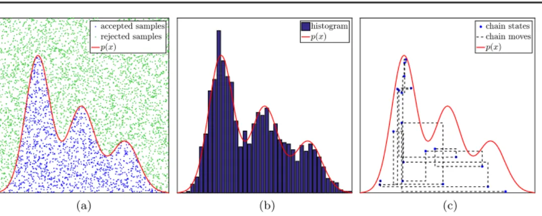
Figure 2.An illustration of accept–reject methods and slice sampling:(a)to sample from the density p x( )(red line), uniform samples₍x yi, i₎₍_{blue and green dots}₎ _are

generated in a region enclosing its graph. All samples fulﬁllingyip x_{( )}i ₍_{blue dots}₎

are accepted.(b)Histogram computed from thexvalues of all accepted samples.(c) Slice sampling. The x coordinates of the blue dots are samples of p x( ), while the dashed black line illustrates the path of the sampler onp.

(10)

Algorithm 3. (Slice sampling)

For a univariate densityp x( )µp x p x₁( ) ₂( ), deﬁne an initial statex0_{, a burn-in size}_K

0and sample size

K. Fori=1,¼,K0+K do:

A3.1. Drawyuniform from 0,p xi 2

[ ( )](vertical move). A3.2. Drawxi+1_from_{p x} _ _x

S

1( ) 2y( )(weighted horizontal move).

Discard xi i= K 0 0 { } and use xi i=+K+ K K 1 0 0 { } as a sample of p x( ).

For all the methods presented in this section,p x( )does not need to be normalized. Also note that for simplicity, we refer to algorithm 3 as the‘slice sampler’, hopefully without causing confusion with the one presented in [30], which was included as the ‘basic slice sampler’(algorithm2)here for completeness of the presentation.

2.4. Slice-within-Gibbs sampling for Bayesian inversion

The implicit variable split introduced in algorithm3is appealing ifS₂y={ ∣z p z₂( )y}is a single interval and easy to determine and p x₁( )constrained to an interval is easy to sample from. For the SC posterior densities we consider here, this holds if we split into likelihood plus hard constraints, i.e., p x1( ) =exp(-ax2+bx)[lb ub, ]( )x , and prior parts p x2( ). As the prior terms are unimodal and some even symmetric to zero,S₂yis a single interval and can be determined easily: for(15), we have p x µexp -c xp +d q p

2( ) ( (∣ ∣ ) )and ⎜ ⎟ ⎛ ⎝ ⎜⎛_⎝ ⎞_⎠ ⎞ ⎠ ⎟   -c x +d y x - y -c d exp p q p log . 28 p q 1 p ( (∣ ∣ ) ) ⟺ ∣ ∣ ( ) ( )

For the TV prior,(21), we need to computeS₂ynumerically. However, as the energy ofp x₂( ) is convex,S₂yis a single interval given by the solutions to p x₂( )=y. As the energy of p x₂( ) is also piecewise smooth and can be bounded from below, we can easilyfind starting points for fast, derivative-based root-finding-algorithms. The details are given in appendix A.2. A generalization to other convex, piecewise-smooth energies, such as(17)with suitablep q, , is straight-forward (p =q =1 is a special case as p x₂( )=y can be solved explicitly by a simple scheme). However, ifD VT _{is dense the number terms in the prior energy is large and} this step will become the computational bottleneck of the whole solver. Fortunately, many relevant operators DT such as finite difference operators or dictionaries composed of local patches are sparse in the original basis,V=In.

The likelihood part p x₁( )is a Gaussian withmSS =b (2a)andsSS=1 2a

2 ₍ _{), truncated} to the intervalI=S2y

Ç

[lb ub, ]. For sampling truncated Gaussians, various direct samplers were developed. Our implementation relies on a modiﬁed, more robust, version of[9]. Note that if the sampler is initialized in a feasible pointu0Î_{, the probability of}_I_{being empty or}

a single point is zero in theory. In practice,ﬁnite precision can lead toI={ ˜}, in which casex one has to set xi+1=x_˜_.

Using the slice sampler presented above to sample from ppost(· ∣x_-j,f)in step A1.2 will be called slice-within-Gibbssampling. In principle, it will generate a full Markov chain

xi_j i₌K+ ₊ ~p x_-,f , 29 K K j 1 post s s s s s ,0 ,0 { } ( · ∣ ) ( )

where we subscripted all variables belonging to the inner slice sampler withs. Practically, we only need one sample fromppost( · ∣x_-j,f). We will always initialize the slice sampler with the current valuex_i of the component we want to update. Then, we only have to determine the

(11)

length of the burn-in phaseKs,0 and choose theﬁrst sample of the real run as a sample of

x

-ppost( · ∣ j,f), i.e.,Ks=1.

The correctness and convergence of the slice-within-Gibbs sampler can be established by combining the properties of the slice sampler (algorithm 3)and the general Gibbs sampler

(algorithm 1), which are discussed in[34]. 3. Computed examples

3.1. Computational scenarios

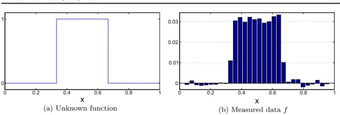
‘Boxcar’—image deblurring in 1D. For the initial evaluation studies, we use a simple image deblurring scenario in 1D that was adopted from [24] and also used in [27]. It is a simpliﬁcation of the task to reconstruct a spatially distributed intensity image that is known to consist of piecewise homogeneous parts with sharp edges: the indicator function of⎡_⎣1₃, 2₃⎤_⎦is to be recovered from its integrals overm=30 equidistant subintervals of[0, 1], corrupted by noise withm=0,S =10-3Im(seeﬁgure 3). The reconstruction is carried out on the grid

= xin

i

256, i=1,¼,n, with n=255 and the forward operator is discretized by the trapezoidal quadrature rule applied to that grid. Further details can be found in section 3.1.1 of [27].

The prior operator DT will be given by the forward difference operator with Neumann boundary conditions: = + - = + - = ¼ -Di ei ei, D ui u u, i 1, ,n 1. 30 T i i 1 ⟹ 1 ( )

DThas full rankh =n -1andVÎRn´n _{given by}

⎧ ⎨ ⎩  = V 1 ifi j, 0 else 31 i j, ( ) ( )

is a basis matrixVsuch thatD VT _{is a diagonal matrix. We will refer to priors based on this} operator asincrement priors. For the ℓ1 increment prior, i.e., the conventional TV prior, we can also use the direct ℓ1sampler to sample from the posterior. By this, we can validate the approximation of the direct SC sampling via iCDF by the slice sampler proposed here. We will refer to this setting as the‘Boxcar’scenario in the following.

‘Phantom-CT’—CT inversion in 2D. We consider an example of 2D sparse angle CT to

demonstrate the potential of the proposed sampler for real-world applications. An approximate model of CT is given by the Radon transform : for a 2D function

(12)

Î -¥

u L2([ 1, 1] ), it computes integrals along straight lines which are parametrized by the2 angle θof their normal vector and their(signed)distance sto the origin:



ò

q q q q q = = + - + q ¥ ¥ -¥ ¥ ¥ u s u x t y t l t u t s t s t , , d

sin cos , cos sin d . 32

l ,s

[ ]( ) ( ( ) ( )) ( )

( ) ( )

( )

In sparse angle tomography, only a small number of such angular projections can be measured. In our study, we chose only mq=45 angles, evenly distributed in[0,p). In

addition, for a given angleqi, we practically only measure the integrals of[u¥](qi,s)over small s-intervals representing an array ofms=500 equal sized sensor pixels. In total, this leads to m=ms·mq=18.000 measurements. The forward operator A corresponds to the

exact discretization of this measurement with respect to the pixel basis: all the operations involved in the measurement can be computed explicitly for indicator functions of rectangular sets. Further details of this step can be found in section 2.3 in[28].

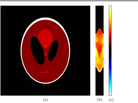
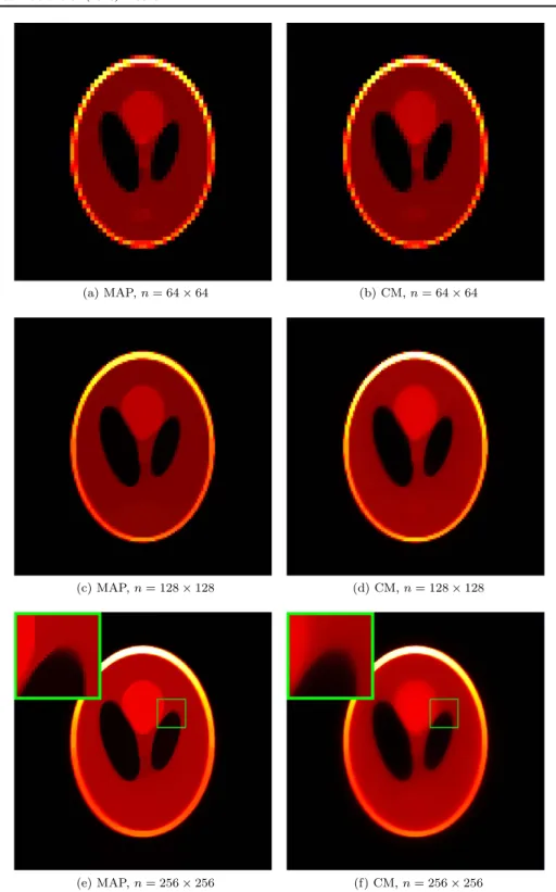
The unknown function u¥ to recover is a slightly scaled version of theShepp–Logan phantom[35], a toy model of the human head deﬁned by 10 ellipses. Figure4(a)showsu¥ and ﬁgure 4(b)the measurement data generated by discretizingu¥ with a 768×768 pixel grid. We will refer to this scenario as‘Phantom-CT’.

3.2. Accuracy assessment

To validate that the developed slice sampler accurately reproduces the distributions it is supposed to sample from, the convergence of the sample histograms to the underlying SC densities was checked for visually. Various (random) combinations of coefﬁcients for the different SC densities were tested; see ﬁgure5 for an example of such a comparison.

Figure 4. ‘Phantom-CT’ scenario. (a) Unknown function to recover. (b) Clean measurement data (‘sinogram’) for ms=500, mq=45. (c) Colormap used for all visulizations in this scenario, 0 corresponds to black.

(13)

3.3. Efficiency assessment

Once the accuracy of the slice sampler is established, the next crucial question is whether its use within a Gibbs sampler isefﬁcient: in algorithm1, we ideally want to replace the current values of the componentj,uiby a values that is both distributed followingppost( · ∣u-j,f)and statistically independent of the current valueui. While direct SC samplers, such as the iCDF,

naturally fulﬁll these requirements, SC samplers relying on MCMC chains initialized withui

fulfill them only asymptotically, in the limit Ks,0  ¥. Using a fixed chain size Ks,0 will inevitably introduce additional correlation between subsequent samples and lower the sta-tistical efficiency of slice-within-Gibbs samplers compared to Gibbs sampling relying on a direct sampler for the SC densities. In the following, we will asses this loss of statistical efficiency by autocorrelation analysis.

Autocorrelation analysis. Evaluating samplers in general rather than for a speciﬁc aim is a difﬁcult task [26]. For the sake of a concise presentation, a detailed introduction and discussion is omitted here but can be found in section 4.1.6. of[28]. In this study, we will only examine the autocorrelation functions of the MCMC chains projected onto a test function vÎn_{, i.e., of the chain}

= = = ++ gi v u, . 33 i K i i K K K 1 0 1 0 { } {⟨ ⟩} ( )

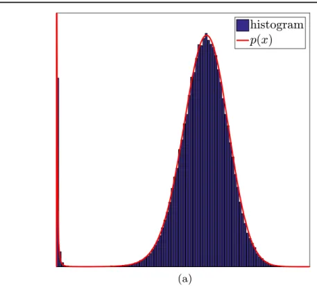
In the‘Boxcar’scenario,vis given as the largest eigenvector of the(pre-computed)posterior covariance matrix while in the‘Phantom-CT’scenario, it is the indicator function of the area Figure 5. (a) Histogram (blue bars) of the slice sampler compared to targeted SC density(red line)given by(16)withp=0.8. The parametersaandbwere picked from a run of the directℓ1sampler applied to a 2D image deblurring scenario(described in

(14)

deﬁned by[-0.32,-0.12]´[0.12, 0.32](this area corresponds to the green box shown in ﬁgures7(e)–(f)). To extract a quantitative measure from the autocorrelation functions, we will estimate their integrated autocorrelation timetint by the approach presented in[41]. In all computed examples, the component j to update in step A1.1 of algorithm 1 is drawn uniformly at random,(random scan Gibbs sampler) and asub-sampling rate (SSR)of n is used, i.e., only everynth sample of the chains generated by algorithm1is actually stored and

t_int refers to the samples of this thinned chain. This means that, on average, we update alln

components of uÎn _{between two steps of the chain} ₍_{full sweep}₎_{. In each scenario, the} samplers were given a large burn-in time K0 and K was chosen large enough to obtain sufﬁciently tight error bounds ontint [41].

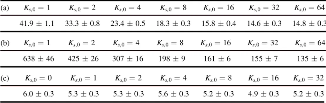
Results. When using a conventional TV prior(p=q=1)in the‘Boxcar’scenario, the direct ℓ1 sampler using the iCDF method can be used as a reference to which the slice samplers can be compared to: thetintobtained by the direct sampler is a lower bound for all slice samplers. Table1lists the results. One can observe that already for small MCMC chain lengthKs,0, the differences between direct and slice sampler in terms of statistical efﬁciency are negligible in practice. Similar examinations usingℓ2priors(where, again, a direct sampler can be used as a reference)showed that in this case, signiﬁcant differences vanish for even smaller values of Ks,0 (results omitted here).

Tables 2(a),(b)and (c) show the results of similar examinations for an ℓp prior with =

p 1.2, anℓpqprior withp=1,q=10 and the isotropic TV prior in the 2D‘Phantom-CT’ scenario (usingn =129 ´129), respectively. While we do not have a direct sampler as a reference here, one can clearly see thatt_intis converging to a limit for increasingK_s,0. In some cases, even using Ks,0=0, i.e., only performing one step of the slice sampler, might be sufﬁcient.

Computational complexity. In typical large scale inverse problems such as the one examined in section3.5, the computational bottleneck is to compute the coefficients of the SC densities, not the process of sampling from them. Therefore, the computational complexity of the slice sampler is not a critical aspect of the whole algorithm. However, to give an indi-cation of how increasingK_s,0effects the total run time, table3compares the run time of the slice-within-Gibbs sampler to the directℓ1sampler and table4lists the run times of the slice-within-Gibbs sampler for the TV prior in 2D. While the implementation of the slice sampling part is more complicated in this situation(see appendixA.2), we see that even for a moderate sized scenario(n=2562₎_{it does not signi}_fi_{cantly effect the run time. Therefore, one does not} have to compromise statistical efficiency by choosing a small Ks,0 to obtain a better com-putational efficiency.

3.4. Application to theℓp increment prior

Problems with the conventional TV prior(see[24]and the overview in section 5.2.2 in[28]) stimulated research into alternative, edge-preserving prior models. Here, we exemplify how the new slice-within-Gibbs sampler can be used to investigate such general questions in Table 1.Comparison oftintfor direct and slice-within-Gibbs samplers using different

burn-in lengths for the slice sampler. The ‘Boxcar’ scenario and a TV prior

(p=q=1)withl=400is used andK=5´106_,_SSR₌_n_.

=

Ks,0 10 Ks,0=20 Ks,0=40 Ks,0=100 Ks,0=200 Direct

(15)

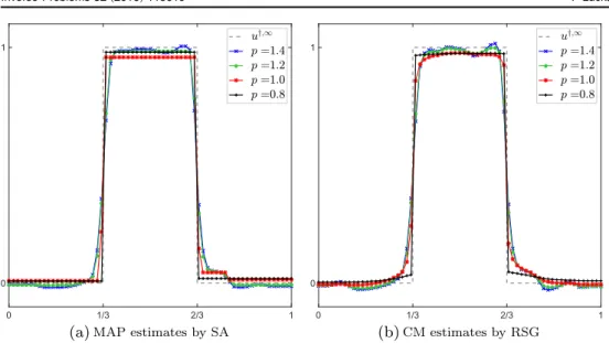
Bayesian inversion: We use it to compute both MAP and CM estimates for theℓpincrement prior with p decreasing from p=2 (Gaussian prior) top=1 (TV prior) and even below

<

p 1(non-logconcave prior). While the computation of the CM estimates is straight-for-ward, computing MAP estimates is done by using the sampler within asimulated annealing (SA) scheme, a stochastic meta-heuristic for global optimization. The details and an eva-luation of using SA together with the proposed SC Gibbs samplers can be found in sections 4.2.4 and 5.1.5 in[28]. In both cases,K=105_{samples were drawn with SSR}₌_n_.

The results of computing MAP and CM estimates for different values ofpare shown in ﬁgure6. Here,λwas chosen such that all likelihood energies are equal and thatl=200for

p=1. The results suggest that using p<1leads to superior results for both MAP and CM estimates compared to p=1. The MAP estimate is closer to the real solution as it is both sparser in the increment basis and the contrast loss is reduced. The CM estimate for p=0.8 looks way more convincing compared to those for p1: it has clear pronounced edges that separate smooth, denoised parts. However, using the slice-within Gibbs samplers for p<1 needs to be examined more carefully: while the results are visually convincing, we cannot be sure that the sampler explored the whole, possibly multimodal posterior and did not get stuck in a single mode.

3.5. Application to CT inversion with TV priors

Figure7shows MAP and CM estimates for the‘Phantom-CT’scenario using an isotropic TV prior with Neumann boundary conditions(19). Here, the MAP estimates were computed with the alternating direction method of multipliers [5]. In the Gibbs sampler, oriented over-relaxation (see [29] and section 4.3.1. in [28]) was used to accelerate convergence and

= ´ ´

K 2.5 10 , 10 , 54 4 103 _{samples were drawn for} _n₌_{64 , 128 , 256}2 2 2_, respec-tively(SSR=n).

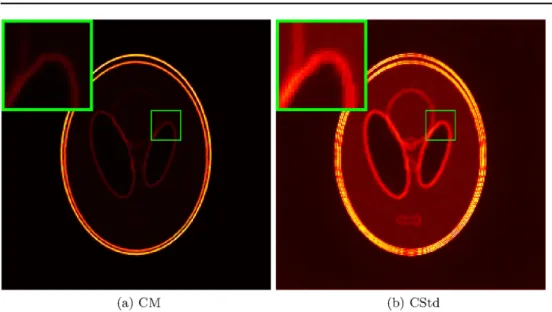
Non-negativity constraints. As the slice-within-Gibbs sampler can easily incorporate

additional hard constraints (10), it can be used to quantify their effect on the posterior p_post( ∣ )u f . Figure8shows CM and CStd estimates computed with or without non-negativity constraints,u 0. While the CM estimates look very similar, the CStd estimates reveal that Table 2. Comparison of tint for slice-within-RSG samplers using different burn-in

lengths for the slice sampler. The‘Boxcar’scenario is used in(a)with anℓpincrement

prior withp=1.2,l=400and in(b)with anℓpqincrement prior withp=1,q=10, l=0.02. In both casesK=2´106_{samples were drawn. In}₍_c₎_{, the}_‘_Phantom-CT_’

scenario with an isotropic TV prior withl=500is used andK=2´105_samples

were drawn. (a) Ks,0=1 Ks,0=2 Ks,0=4 Ks,0=8 Ks,0=16 Ks,0=32 Ks,0=64 41.9±1.1 33.3±0.8 23.4±0.5 18.3±0.3 15.8±0.4 14.6±0.3 14.8±0.3 (b) Ks,0=1 Ks,0=2 Ks,0=4 Ks,0=8 Ks,0=16 Ks,0=32 Ks,0=64 638±46 425±26 307±16 198±9 161±6 155±7 135±6 (c) Ks,0=0 Ks,0=1 Ks,0=2 Ks,0=4 Ks,0=8 Ks,0=16 Ks,0=32 6.0±0.3 5.3±0.3 5.3±0.3 5.6±0.3 5.2±0.3 4.9±0.3 5.2±0.3

(16)

the non-negativity constraints lead to a signiﬁcant reduction of the posterior variance in some regions.

Gradient estimates. we further present one example of how the samples ofugenerated by

the sampler can be used to compute statistics and uncertainties of a feature of u (see section1.2): inﬁgure9(a), we computed the CM estimate of the gradient of the imageu

[u2∣ ]f =

_ò

u2 ppost( ∣ )u f du (34) and ﬁgure9(b)shows the corresponding CStd estimate.

Figure 6.MAP and CM estimates for the 1D‘Boxcar’scenario using theℓpincrement

prior andn=63. The true function to recover(gray line plot)is denoted byu†,¥_.

Table 3. Total run time of the slice-within-Gibbs sampler using different burn-in lengths divided by the run time of the directℓ1sampler. The‘Boxcar’scenario and anℓp

increment prior with p=1.2,l=400 is used. =

Ks,0 10 Ks,0=20 Ks,0=40 Ks,0=100 Ks,0=200

1.30 1.38 1.48 1.75 2.20

Table 4. Total run time of the slice-within-Gibbs sampler using different burn-in lengths Ks,0 divided by the run time for Ks,0=0. The ‘Phantom-CT’ scenario (n=256´256)and a TV prior(p=1)withl=500is used.

=

Ks,0 0 Ks,0=1 Ks,0=2 Ks,0=4 Ks,0=8 Ks,0=16 Ks,0=32

(17)

Figure 7.MAP and CM estimates for the‘Phantom-CT’scenario using an isotropic TV prior with l=500, computed with increasing spatial resolution. In the highest resolution, a zoom inset is added.

(18)

4. Discussion and conclusions

In this article, we presented and evaluated a new MCMC sampler that allows us to carry out sample-based Bayesian inversion for a wide range of scenarios and prior models. It is based on the extension of the SC Gibbs-type sampler developed in [27] by a problem-specific adaptation and implementation of generalized slice sampling and enables efficient posterior sampling in high-dimensional scenarios with certain priors for the first time.

The results in sections3.2and3.3show that using generalized slice sampling to sample from the one-dimensional conditional, SC densities can lead to a fast, robust and accurate Figure 8.Inﬂuence of inculding non-negativity constraints on CM and CStd estimates in the‘Phantom-CT’scenario using an isotropic TV prior withl=50 and a spatial resolution of n=256´256. A zoom inset is added and both CM and both CStd estimates share the same color scale.

(19)

posterior sampler for the inverse problems scenario (1)and is therefore an attractive option whenever a fast direct sampler such as iCDF is not available. The computed results in section 3.4 exempliﬁed the use of the new slice-within-Gibbs sampler to examine recent topics in Bayesian inversion and section 3.5 demonstrated how it can lead to interesting results for Bayesian estimation in challenging, high-dimensional inverse problems scenarios. In particular, we examined that TV prior model in 2D: the theoretical analysis of the TV prior carried out, e.g. in [23,24], is restricted to 1D, only, and, to the best of our knowledge, no theoretical results are available for higher dimensions, yet. The development of the slice-within-Gibbs sampler now enabled us to examine the use the TV prior for the important inverse problem scenario of CT inversion in 2D, for the ﬁrst time. The results show that, contrary to the 1D case, the CM estimates seem to get smoother for a constant value ofλas the resolution increases. This observation could be the starting point for a new theoretical analysis and has to be examined in higher spatial dimensions by computational studies.

More generally, while our results and those of others(see section1.2)have demonstrated that sampling high-dimensional posterior distributions is feasible for many important inverse problems scenarios nowadays, an important future challenge lies in extracting the information of interest from the samples generated: while we demonstrated, e.g., how to compute CStd estimates to examine how the posterior variance is inﬂuenced by non-negativity constraints

(seeﬁgure8)or estimates of a feature g u( )of u (seeﬁgure 9), we did not discuss how to interpret the corresponding results. This requires a concrete application and objective and will be topic of future investigations based on the methods presented here.

Related to the last point, we only used simulated data scenarios in this study to focus on the sampling algorithm. The application to experimental CT data will be the subject of a forthcoming publication covering more general aspects of Bayesian inversion in practical applications (see section 5.3. in [28]). Furthermore, only prior models based on ℓ_pq-norms were considered here, while the sampler can, in principle, be implemented for more general prior models. A more fundamental limitation and future challenge is the current restriction to Figure 9.CM and CStd estimates ofu2for the‘Phantom-CT’scenario using an

isotropic TV prior withl=50, non-negativity constraints and a spatial resolution of

= ´

(20)

linear forward maps (1)and Gaussian noise models(2). Both nonlinear forward maps and non-Gaussian noise models typically conflict with condition (SC1), i.e., they make it very difficult tofind an explicit parameterization of the SC densities. In addition, problems related to using SC-Gibbs sampling for multimodal posteriors(see section3.4)may occur as well. Code to reproduce all the computed examples will be provided as part of the release of a Matlab-based toolbox for Bayesian inversion.

Acknowledgments

This work was conducted as part of the PhD thesis [28]at the University of Münster. The author would like to thank the two supervisors, Martin Burger and Carsten H Wolters. Appendix A. Details of the implementation

A.1. Computation of the likelihood coefficients

To implement the SC Gibbs sampler for the‘Boxcar’scenario, we computeY =AVand pre-compute a  Yi

1

2 2

2

≔ . For computing b = YTij( )i = Y - Y YTif ( Ti -i)x-i, we pre-compute Y_iTf and yi 2

2_{for all}_i_{and build the}_n__×__n_matrix_F_≔_{Y Y}t _{. Then, computing} _{Y Y} _x

- -i T i i ( ) can be performed by using x x x y Y Yi - - = F -   , A.1 t i i t ,i i i 22 ( [ ]) [ ] (· ) ( )

which involves a scalar product of dimensionn as the most expensive operation.

For the‘Phantom-CT’scenario, there are two possible implementations: For the image sizes considered here (n up to 256×256)we can still compute the matrices Y =A and F_≔ Y Yt _{explicitly and use the same implementation as in the}_‘_Boxcar_’_scenario₍_{Y =}_A_as we stay in the pixel basis, i.e.,V=In). For largernor 3D applications, we might not be able to store Φ or Ψ. An alternative implementation that does not require storing any matrices uses

x x

= Y - Y Y +  Y

b iTf iT( ) i i 22 (A.2)

to computebin the following way:

• We again pre-computeYT_if and Yi 22for alli. Then, we store the measurement that the current stateξwould cause asf_ξand initialize it byAu0_{. In principle,}_f

ξis given asYx, and can be directly computed at any time but this computation is too expensive to be performed at every SC update.

• For a given pixelithat is to be updated, we constructYiand compute the scalar product Y_iTf_x to updateb by the above formula(note thatYiT(f- Yx) is just a projection ofYi onto the current residual of f_x = Yx). With the constructedYi and the change,di, inxi caused by the sampling step, we can then update f_x =f_x + Ydi i.

• While this iterative updating off_ξis fast, inaccuracies can accumulate over time, leading to a misﬁt betweenf_ξandYx. Therefore, we computeYxexplicitly everynsteps and reset

f_ξto this exact value.

The computational bottleneck of this procedure is to computeYi, i.e., the Radon transform of a pixel(or voxel in 3D). For the parallel beam geometry used here, explicit formulas relying on basic operations that can be parallelized over the angles θ can be derived. For more complicated beam geometries, e.g., the cone beam geometry for 3D reconstruction,

(21)

approximations relying on basic operations from computer graphics can be derived and implemented very efﬁciently and parallelized on GPUs.

A.2. Slice sampling with TV priors From (21), we have ⎛ ⎝ ⎜⎜ ⎞ ⎠ ⎟⎟ 

å

= - - + Î = p x exp c d x e g , d 0, 1, 2 , g 0 A.3 j j j j j j 2 1 3 2 ( ) ( ) { } ( )

and want to determineS₂y={ ∣z p z₂( )y}by solving

å

= - = - + = A.4 y p x y c d x e g log , j j j j 2 1 3 2 ₍ ₎ ( ) ⟺ ( ) ( )

where yÎ(0,p x2( ))with probability 1 and p x2( ) 1. Assume that{e e1, 2,e3}are sorted and deﬁne J xj d xj -ej +gj

2

( ) ≔ ( ) and h ≔ -log( )y c. Then, J x( ) ≔ å_jJ xj( ) is convex and smooth inI1 ≔ (-¥,e1),I2 ≔ (e e1, 2),I3 ≔ (e2,e3)andI4 ≔ (e3,¥). It is monotonic in I1 and I4 and is bounded from below by b x( ) ≔ åj d xj∣ -ej∣. Deﬁne

* * =

- +

x ,x argminJ x

[ ] ( ) as the interval of minimizers and x-, x+ as the solutions to =

y p x₂( ). We have x-<x-*, x+>x+*, x-ÎI1

È È

I2 I3 and x+ÎI2

È È

I3 I4 with probability 1 and[x_-*,x₊*]Ì[e e1, 3]. SeeﬁgureA1 for two illustrations.

We will compute x-by a Newtonʼs method:

= - -¢ - -- -- -x x J x h J x , A.5 i i i i 1 1 1 ( ) ( ) ( )

Figure A1.Illustration of two SC density energies for the slice sampler implementation of the TV prior in 2D:J x( )(blue line),b x( )(red line)andh(green and yellow lines) for (e e1, 2,e3)= -( 1, 0, 1) and (a) (d d1, 2,d3)=(2, 1, 1 ,) (g g g1, 2, 3)=(0, 0.5, 1), (b)(d d1, 2,d3)=(1, 0, 1 ,) (g g g1, 2, 3)=(0, 0, 0).

(22)

initialized in a point x_-0 such thatx_-0x-andJ x( )is smooth on[x-0,x-]. In each step, the Newtonʼs method approximatesJ x( )by a tangent inx_-i-1. Due to the convexity ofJ x( )and

*

 <

- -

-x0 x x , the iterates never overshoot: x-0x-i x-for all i. Thereby, they stay in

-

-x0,x

[ ] and the derivative exists. Finding such an initialization x-0 requires some simple considerations:

The subdifferential¶J x( ) is given as the sum of the subdifferentials ofJ xi( ) (in the set-valued sense of addition):

⎧ ⎨ ⎪ ⎪ ⎩ ⎪ ⎪ ⎧ ⎨ ⎪ ⎩⎪ ⎫ ⎬ ⎪ ⎭⎪ ¶ = -- + ¹ > - = = J x d x e d x e g x e g d d x e g , if or 0, , , if and 0. A.6 j j j j j j j j j j 2 ( ) ( ) ( ) [ ] ( )

Now, let Je* ≔ minjJ e( ). We can distinguish two cases:j

*

>

h Je: in this case, we check the following conditions in sequence:

• Ifh >J e1( ),x-is inI1. We use the lower boundb x( ) to determinex-0 such thatb x( _-0)=h:

å

= + -x e J e h d A.7 j j 0 1 1 ( ) ( ) Asb x( )J x( ), and both are monotonic inI1, we have thatx-0<x-.

• Else ifh>J e( ),2 x-is inI2. We perform one Newton step frome1using the maximal subgradient ine1: = - -¶ -x e J e h J e max A.8 0 1 1 1 ( ) ( ( )) ( )

This way,x_-0x-and[x-0,x-]ÌI2, i.e.,J x( )is differentiable for all iterates. • Else,h>J e( )3 and x-is inI3. With a similar reasoning, we set

= - -¶ -x e J e h J e max . A.9 0 2 2 2 ( ) ( ( )) ( )

For ﬁnding x+, a similar reasoning can be applied. In the locations of non-differentiability, the minimal subgradient has to be used.

*

<

h Je: in this case,J x( )is not piecewise linear(see the yellow line inﬁgure9(a))and the unique minimizerx*is not in{e e1, 2,e3}. The convexity ensures thatx-<x*<x+ are all either inI2orI3. Ifmax(¶J e( ))1 <0andmin(¶J e( ))2 >0we have thatx*

(and thereby x-andx+)are inI2. Otherwise, they are inI3. As above, initial points

-x0 and x+0 fulﬁlling the conditions can be found by performing one Newton step from the corners of the interval using the maximal/minimal subgradient.

The case h=Je*has probability zero. References

[1] Agapiou S, Bardsley J M, Papaspiliopoulos O and Stuart A M 2014 Analysis of the Gibbs sampler for hierarchical inverse problemsSIAM/ASA J. Uncertain. Quantiﬁcation2511–44

[2] Bardsley J M 2012 MCMC-Based Image reconstruction with uncertainty quantiﬁcationSIAM J. Sci. Comput.34A1316–32

(23)

[3] Bardsley J M and Fox C 2012 An MCMC method for uncertainty quantiﬁcation in nonnegativity constrained inverse problemsInverse Problems Sci. Eng.20477–98

[4] Bardsley J M, Solonen A, Haario H and Laine M 2014 Randomize-then-optimize: a method for sampling from posterior distributions in nonlinear inverse problemsSIAM J. Sci. Comput.36 A1895–910

[5] Boyd S, Parikh N, Chu E, Peleato B and Eckstein J 2011 Distributed optimization and statistical learning via the alternating direction method of multipliersFound. Trends Mach. Learn.31–22

[6] Burger M and Lucka F 2014 Maximuma posterioriestimates in linear inverse problems with log-concave priors are proper Bayes estimatorsInverse Problems30114004

[7] Calvetti D, Kaipio J P and Somersalo E 2014 Inverse problems in the Bayesian frameworkInverse Problems30110301

[8] Candes E, Romberg J and Tao T 2006 Robust uncertainty principles: exact signal reconstruction from highly incomplete frequency informationIEEE Trans. Inf. Theory52489–509

[9] Chopin N 2011 Fast simulation of truncated Gaussian distributionsStat. Comput.21275–88 [10] Comelli S 2011 A novel class of priors for edge-preserving methods in Bayesian inversion

Master’s ThesisUniversity of Milan, Italy

[11] Cui T, Fox C and O’Sullivan M J 2011 Bayesian calibration of a large-scale geothermal reservoir model by a new adaptive delayed acceptance Metropolis Hastings algorithmWater Resour. Res.

47W10521

[12] Cui T, Law K J and Marzouk Y M 2016 Dimension-independent likelihood-informed MCMC

J. Comput. Phys.304109–37

[13] Dashti M, Harris S and Stuart A 2012 Besov priors for Bayesian inverse problems Inverse Problems Imag.6183–200

[14] Donoho D L 2006 Compressed sensingIEEE Trans. Inf. Theory521289–306

[15] Foucart S and Rauhut H 2013 A Mathematical Introduction to Compressive Sensing (Basel: Birkhäuser)

[16] Haario H, Laine M, Mira A and Saksman E 2006 DRAM: efﬁcient adaptive MCMCStat. Comput.

16339–54

[17] Haario H, Saksman E and Tamminen J 2005 Componentwise adaptation for high dimensional MCMCComput Stat.20265–73

[18] Hämäläinen K, Kallonen A, Kolehmainen V, Lassas M, Niinimaki K and Siltanen S 2013 Sparse tomographySIAM J. Sci. Comput.35B644–65

[19] Helin T and Burger M 2015 Maximuma posterioriprobability estimates in inﬁnite-dimensional Bayesian inverse problemsInverse Problems31085009

[20] Kaipio J P and Somersalo E 2005 Statistical and Computational Inverse Problems (Applied Mathematical Sciencesvol 160) (New York: Springer)

[21] Kolehmainen V, Lassas M, Niinimäki K and Siltanen S 2012 Sparsity-promoting Bayesian inversionInverse Problems28025005

[22] Lanfer B 2014 Automatic generation of volume conductor models of the human head for EEG source analysisPhD ThesisUniversity of Muenster

[23] Lassas M, Saksman E and Siltanen S 2009 Discretization invariant Bayesian inversion and Besov space priorsInverse Problems Imag.387–122

[24] Lassas M and Siltanen S 2004 Can one use total variation prior for edge-preserving Bayesian inversion?Inverse Problems201537–63

[25] Latuszynski K, Roberts G O and Rosenthal J S 2013 Adaptive Gibbs samplers and related MCMC methodsAnnal. Appl. Probab.2366–98

[26] Liu J 2008Monte Carlo Strategies in Scientiﬁc Computing(Springer Series in Statistics) (New York: Springer)

[27] Lucka F 2012 Fast Markov chain Monte Carlo sampling for sparse Bayesian inference in high-dimensional inverse problems using L1-type priorsInverse Problems28125012

[28] Lucka F 2014 Bayesian inversion in biomedical imagingPhD ThesisUniversity of Münster [29] Neal R M 1995 Suppressing random walks in Markov chain Monte Carlo using ordered

overrelaxationTechnical Report9508 Learning in Graphical Models [30] Neal R M 2003 Slice samplingAnn. Stat.31705–67

[31] Palafox A, Capistran M A and Christen J A 2014 Effective parameter dimension via Bayesian model selection in the inverse acoustic scattering problemMath. Problems Eng.201412 [32] Pereyra M 2015 Proximal Markov chain Monte Carlo algorithmsStat. Comput.26745–60

(24)

[33] Pereyra M, Schniter P, Chouzenoux E, Pesquet J-C, Tourneret J-Y, Hero A and McLaughlin S 2016 A Survey of stochastic simulation and optimization methods in signal processingIEEE J. Sel. Top. Signal Process.10224–41

[34] Robert C P and Casella G 2005Monte Carlo Statistical Methods(Springer Texts in Statistics) (New York: Springer)

[35] Shepp L and Logan B 1974 The fourier reconstruction of a head sectionIEEE Trans. Nucl. Sci.21 21–43

[36] Cotter S L, Roberts G O, Stuart A and White D 2013 MCMC methods for functions: modifying old algorithms to make them fasterStat. Sci.28424–46

[37] Sommariva S and Sorrentino A 2014 Sequential Monte Carlo samplers for semi-linear inverse problems and application to magnetoencephalographyInverse Problems30114020

[38] Sorrentino A, Luria G and Aramini R 2014 Bayesian multi-dipole modelling of a single topography in MEG by adaptive sequential Monte Carlo samplersInverse Problems30045010 [39] Stuart A M 2010 Inverse problems: a Bayesian perspectiveActa Numer.19451–559

[40] Vogel C R 2002 Computational Methods for Inverse Problems(Philadelphia, PA: Society for Industrial and Applied Mathematics)