Capacity Analysis of Signalised Intersections in Motorcycle Dependent Cities

Capacity Analysis of

Signalised Intersections in

Motorcycle Dependent Cities

M.Eng. Huynh Duc Nguyen

A dissertation submitted in fulfilment of the requirements for the Degree of Doktor-Ingenieur (Dr.-Ing.) of the Department of Civil and Environmental Engineering, Technische Universität Darmstadt.

Supervisor: Prof. Dr.-Ing. Manfred Boltze Technische Universität Darmstadt, Germany Co-supervisor: Prof. Dr. Eng. Hideki Nakamura Nagoya University, Japan Date of submission: 16.10.2018 Date of oral examination: 11.02.2019

Nguyen, Huynh Duc

Capacity Analysis of Signalised Intersections in Motorcycle Dependent Cities

Herausgeber:

Technische Universität Darmstadt

Institut für Verkehrsplanung und Verkehrstechnik Otto-Berndt-Str. 2

64287 Darmstadt

www.tu-darmstadt.de/verkehr [email protected]

Schriftenreihe der Instituts für Verkehr

Institut für Verkehrsplanung und Verkehrstechnik Heft V43

ISSN 1613-8317

Year thesis published in Tuprints 2020 Date of the viva voce 11.02.2019

Published under CC BY-SA 4.0 International https://creativecommons.org/licenses/

i

Acknowledgement

First, I would like to express my sincere appreciation to the co-operation program between Vietnamese-German Transport Research Centre, Vietnamese-German University, Vietnam and Technische Universität Darmstadt, Germany. I had an opportunity to conduct this study thanks to this program.

I also would like to express my thanks to the Ministry of Education and Training of Vietnam (MOET) and relevant agencies for supporting me with the 911 scholarship during my study at Darmstadt University of Technology.

Especially, I would like to express my sincere gratitude to Professor Dr.-Ing. Manfred Boltze, Head of the Institute of Transport Planning and Traffic Engineering, Technische Universität Darmstadt, Germany, as the first supervisor of my work. Without his supervision, I would not have completed this research. It is also very lucky for me to send my sincere thanks to the co-supervisor, Prof. Dr. Eng. Hideki Nakamura, as the second supervisor of my work. He discussed and gave me valuable recommendations with his experiences.

I would like to appreciate Dr. Vu Anh Tuan, director of the VGTRC, for his support in discussing and giving comments of my research. I also want to give grateful thanks to Dr. Chu Cong Minh, the former executive manager of VGTRC, and Dr. Khuat Viet Hung, the former co-director of VGTRC. They introduced me to the doctoral program and supported me to fulfil the requirements and the acceptance by Professor Dr.-Ing. Manfred Boltze.

My sincere gratitudes are directed to my colleagues in VGTRC, TU Darmstadt and other friends from Nagoya University, Tongji University and Indian Institute of Technology Kharagpur. They never hesitated to give me feedbacks and discussions from their point of view. That great working environment is a success factor to my completion.

I’m very lucky to have help from the secretary, students and other relevant people at Darmstadt during my stay there. I would like to give my thanks for all their help.

Finally, I would like to express my appreciation towards my family members. Without their encouragement, sympathy and support, I cannot complete my dream and finish this dissertation.

ii

Abstract

The capacity of a traffic stream is one of the most significant parts of traffic performance analysis. Particularly, capacity analysis of signalised intersections has been studied in developed countries where the primary transportation mode is the private car usage. In some developing countries, however, there are several distinctive traffic flow characteristics in contrast with those in developed countries such as 80% of traffic composition being motorcycles, which is leading to the term ‘Motorcycle Dependent City (MDC)’. Moreover, motorcycle driving behaviour in MDCs is entirely different from four-wheeled vehicle driving behaviour in car dependent cities. Therefore, we cannot use models defined for car traffic in developed countries to analyse performances of motorcycle traffic and to evaluate the capacities of signalised intersections in developing countries such as Vietnam. This research focuses on proposing suitable models which can explain the specific characteristics of traffic streams in MDCs and the intersection capacities in different traffic situations. This goal can be divided into objectives: finding factors that affect the capacity of signalised intersections significantly; proposing a suitable capacity calculation method; developing a capacity calculation guideline for signalised intersections in MDCs. However, the research area of this study is limited to the concept of MDCs in which the motorcycle occupies a high share in traffic composition.

The comprehensive literature review on the capacity of signalised intersections is conducted in both, car dependent cities and motorcycle dependent cities, to understand the calculation method throughout various countries. Several methods and manuals in car traffic-based conditions such as German Highway Capacity Manual (HBS) (FGSV, 2015), American Highway Capacity Manual (HCM) (TRB 2010), Indonesia Highway Capacity Manual 1997 (IHCM 1997), Malaysia Highway Capacity Manual 2011 (MHCM 2011) and the Manual on Traffic Signal Control in 2006 (JSTE 2006) are introduced. Besides, some models from researched projects in MDCs are mentioned to indicate the difference in traffic situations between these cities and others. Basically, the capacity of signalised intersections includes two main components: the saturation flow rate and the effective green ratio. The saturation flow rate would be calculated by the base saturation flow rate and is adjusted by some influencing factors. Depending on the characteristics of each location and the selected method, the saturation flow rate analysis process may differ from car traffic-based flow to motorcycle traffic-based flow. In this study, the saturation flow rate models would also follow the common concept of previous studies. The base saturation flow rate will be investigated, and the motorcycle unit will be used as the basic unit. Then some main adjustment factor will be applied for the model such as approach width, vehicle type, turning activities, etc. On the other hand, the effective green ratio shows the correlation between the effective green time and the cycle time. In car traffic-based flow, the effective green time has been proved to be 1 s higher than the displayed green time. However, in MDCs, this outcome is still a controversial question and is needed to be evaluated because of its unique traffic characteristics. The traffic characteristics at signalised intersections in MDCs are analysed to figure out how they affect the intersection capacity. The traffic characteristics are categorised into several factors: vehicle characteristics, volume characteristics, speed characteristics, lane allocation characteristics, traffic signal systems, and driver behaviour. From the literature review and the traffic characteristics which are mentioned, the overall capacity model for MDCs is built up as the combination of the saturation flow rate model, the effective green time model, and the intergreen time model. The normal capacity and the maximum capacity are estimated depending on the different effective green times. Besides the proposed theoretical models, field observations are also conducted in Ho Chi Minh City, Vietnam for the model calibration process. The contents and the researching results of each model can be summarised as follows:

iii

After proposing the comprehensive capacity model of signalised intersections, a procedure for application of that model and a sample calculation are introduced. The procedure for application is presented as a guideline which depicts step by step capacity calculation at signalised intersections in MDCs for operational and planning purposes. Finally, this research concludes with recommendations, limitations, and further studies.

• The saturation flow rate is estimated by the motorcycle saturation flow rate and adjustment factors. In the model, the term ‘normalised saturation flow rate’ which is defined as the saturation flow rate passing over one-meter approach width is introduced. Observation results showed that the normalised saturation flow rate was calculated at 3,058 mcu/(h*m) when the green time was higher or equal to 16 s. That rate was estimated at 3,178 mcu/(h*m) when the green time was lower than 16 s.

• Motorcycle equivalent unit (MCU) is chosen as a basic unit to apply the conversion of heterogeneous streams to homogeneous motorcycle streams. The MCU values may vary depending on the share of passenger cars in the flow. The MCU value changes from 5.5 to 6.8 corresponding with the car share value of 5% to 100%. The recommended MCU values for cars, middle heavy vehicles and heavy vehicles for normal calculation are 6, 9 and 14.4, respectively. • Besides the adjustment factor for the approach width, the adjustment factors for vehicle types and

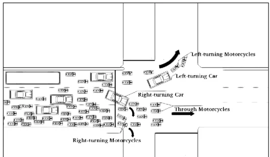
turning movements are considered as the main affecting factors of the saturation flow rate model. The numerical results indicated that the impact of vehicle type was the primary factor and contributed to reducing the approach capacity significantly. As regards the effect of turning movements, different turning types have different effects on the approach capacity. Right-turning motorcycles do not influence the discharge flow rate because they are assigned to run on the right side of the flow. Right-turning cars, however, affect the through-flow significantly because of their left-side position. Left-turning motorcycles interfere through-discharging cars and left-turning cars, and they would reduce the discharging speed of through-vehicles.

• The effective green time model applies a method to count the number of motorcycles passing the stop line during certain time periods. Two models are classified: model 1 when the rule ‘no red-light running’ is strictly obeyed and model 2 when the rule ‘no red-red-light running’ is ignored. In the first model, the effective green time was proven to be equal to the displayed green time. In the second model, the effective green time was estimated to be equal to the displayed green time plus 2 s.

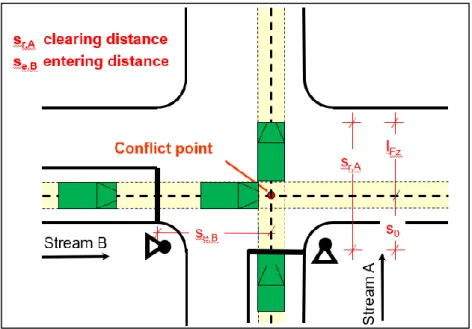
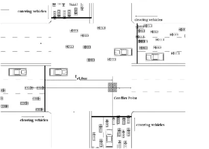
• The intergreen time model in MDCs applies the German method with some modifications. The crossing time was recommended to be equal to the amber time which is set up at 3 s for most cases. The clearing time was increased by the addition of the interaction time between clearing through-vehicles and clearing opposing left-turning movements. The interaction time depends on vehicle types at each stream and was suggested as 1 s. The entering time was calculated by the entering distance which was defined from the middle point of the stop line to the centre of the conflict area between the entering route and the clearing route, and the entering speed was observed as 5 m/s.

• The normal capacity and the maximum capacity are estimated depending on the different effective green times. The normal capacity is presented along with the rule ‘no red-light running’ which drivers must obey. Besides, the maximum capacity is given along with weak acceptance of the rule ‘no red-light running’ which is ignored by many drivers, in practice. In this thesis, the normal capacity is recommended for the capacity analysis. The maximum capacity is considered as an adaption to the current traffic situation while the illegal driving behaviour could not be controlled.

iv

Kurzfassung

Die Kapazität eines Verkehrsstroms ist einer der Hauptbestandteile zur Analyse der Leistungsfähigkeit im Verkehr. In entwickelten Ländern, in denen das primäre Verkehrsmittel das private Automobil ist, wurde insbesondere die Kapazitätsanalyse von signalisierten Knotenpunkten analysiert. In einigen Entwicklungsländern gibt es mehrere Besonderheiten gegenüber entwickelten Ländern im Verkehrsablauf, wie ein 80-prozentiger Verkehrsanteil von Motorrädern. Daher wurde der Begriff der motorradabhängigen Stadt / Motorcycle Dependent City (MDC) eingeführt. Außerdem unterscheidet sich das Fahrerverhalten von Kraftradfahrern in MDC sehr stark von dem Fahrerverhalten vierrädriger Fahrzeuge in autoabhängigen Städten. Deshalb können Modelle, die für die Analyse des Autoverkehrs bestimmt sind, nicht verwenden werden um die Leistungsfähigkeit des Motorradverkehrs zu analysieren und die Kapazität von signalisierten Knotenpunkten in Entwicklungsländern wie Vietnam zu beurteilen.

Diese Arbeit soll geeignete Modelle erarbeiten, die spezifische Charakteristika von Verkehrsströmen in MDCs berücksichtigen und Kapazitäten von Knotenpunkten in verschiedenen Verkehrssituationen erklären können. Das Ziel der Arbeit kann in folgende Unterziele aufgeteilt werden: Vorschlag einer geeigneten Kapazitätsberechnungsmethode; Identifizierung von Faktoren, durch die die Kapazität von signalisierten Knotenpunkten signifikant beeinflusst wird; Datenerhebung durch Feldbeobachtungen; Analyse von Knotenpunktkapazitäten in MDCs; Entwicklung eines Leitfadens für signalisierte Knotenpunkte in MDCs. Das Untersuchungsgebiet dieser Arbeit beschränkt sich auf MDCs in denen Motorräder einen sehr hohen Verkehrsanteil einnehmen.

Die umfassende Literaturrecherche zur Kapazitätsbetrachtung von signalisierten Knotenpunken wurde sowohl für autoabhängige Städte als auch für motorradabhängige Städte durchgeführt, um ein Verständnis für die Berechnungsmethoden in verschiedenen Ländern zu entwickeln. Eine Vielzahl von Methoden und Handbüchern für Autoverkehr, wie das deutsche Handbuch für die Bemessung von Straßenverkehrsanlagen (HBS) (FGSV, 2015), das US-amerikanische Highway Capacity Manual (HCM) (TRB 2010), das indonesische Highway Capacity Manual 1997 (IHCM 1997), das malaysische Highway Capacity Manual 2011 (MHCM 2011), und das Manual on Traffic Signal Control von 2006 (JSTE 2006) werden vorgestellt. Zudem werden Modelle von Forschungsprojekten in MDCs dargestellt, um die Unterschiede der verschiedenen Verkehrssituationen in diesen und anderen Städten zu verdeutlichen. Grundsätzlich umfasst die Kapazität von signalisierten Knotenpunkten zwei Hauptkomponenten: Die resultierende Sättigungsverkehrsstärke und den effektiven Freigabezeitanteil. Die resultierende Sättigungsverkehrsstärke wird berechnet über die Sättigungsverkehrsstärke bei Standardbedingungen und zugehörige Abminderungsfaktoren. Abhängig von örtlichen Gegebenheiten und der verwendeten Methode kann sich der Prozess zur Bestimmung der Sättigungsverkehrsstärke zwischen autobasiertem Verkehrsfluss und motorradbasiertem Verkehrsfluss unterscheiden. In dieser Arbeit sollen die Modelle zur Bestimmung der Sättigungsverkehrsstärke dem grundlegenden Konzept früherer Studien folgen. Die Sättigungsverkehrsstärke bei Standardbedingungen wird untersucht, und Motorräder werden als Basiseinheit zur Homogenisierung des Verkehrsflusses verwendet. Danach wurde einige primäre Anpassungsfaktoren, wie Zufahrtsbreite, Fahrzeugtyp, Abbiegevorgänge auf das Modell angewendet. Der effektive Freigabezeitanteil beschreibt das Verhältnis zwischen der effektiven Freigabezeit und der Umlaufzeit. Im autobasierten Verkehrsfluss wurde nachgewiesen, dass die effektive Freigabezeit 1s höher ist als die angezeigte Grünzeit. Allerdings ist dieses Ergebnis für MDCs noch umstritten, und es besteht aufgrund der besonderen Verkehrscharakteristika die Notwendigkeit, dies zu evaluieren. Die Verkehrseigenschaften an signalisierten Knotenpunkten in MDCs werden analysiert, um herauszufinden, welchen Effekt sie auf die Kapazität von Knotenpunkten haben. Die Verkehrseigenschaften werden wie folgt kategorisiert: Fahrzeugeigenschaften, Verkehrstärken, Geschwindigkeiten, Fahrstreifenzuordnung, Lichtsignalsysteme und Fahrerverhalten. Auf Grundlage

v

der Literaturanalyse und den Verkehrseigenschaften wird das übergreifende Kapazitätsmodel für MDCs aus einer Kombination des Sättigungsverkehrsstärkenmodells, des Modells der effektiven Freigabezeit und des Zwischenzeitenmodells aufgebaut. Die Standardkapazität und die maximale Kapazität werden abhängig von den unterschiedlichen effektiven Freigabezeiten geschätzt. Neben dem vorgeschlagenen theoretischen Modell werden Feldbeobachtungen für den Kalibrierungsprozess des Modells in Ho Chi Minh City (Vietnam) durchgeführt. Die Inhalte und die Forschungsergebnisse zur Modellierung können wie folgt zusammengefasst werden:

• Die Sättigungsverkehrsstärke wird über die Sättigungsverkehrsstärke der Motorräder und die Anpassungsfaktoren bestimmt. Im Modell wird der Term „normalisierte Sättigungsverkehrsstärke’ eingeführt als die Sättigungsverkehrsstärke für einen Meter Zufahrtsbreite, da die Sättigungsverkehrsstärke pro Fahrstreifen in MDCs nicht geeignet für die Berechnung ist. Beobachtungsergebnisse haben gezeigt, dass sich eine normalisierte homogene Flussrate von Krafträdern von 3058 mcu/(h*m) während einer Freigabezeit größer oder gleich 16 s ergibt. Bei einer Freigabezeit von weniger als 16 s ergibt sich ein Wert von 3178 mcu/(h*m).

• Die Motorradeinheit (MCU) wurde als Basiseinheit in dieser Arbeit gewählt, um heterogene Ströme in homogene Ströme von Krafträdern umzurechnen. Die MCU-Äquivalenzwerte können aufgrund der Anteile von Autos im Verkehrsstrom variieren. Der MCU-Äquivalenzwert schwankt zwischen 5,5 und 6,8 in Abhängigkeit vom Verkehrsanteil der Autos von 5% bis 100%. Der empfohlene MCU-Äquivalenzwert für Autos, Minibusse und Busse beträgt jeweils 6,9 und 14,4.

• Neben dem Anpassungsfaktor für die Zufahrtsbreite zählen der Anpassungsfaktor für die Fahrzeugtypen und der Anpassungsfaktor für Abbiegevorgänge zu den primären Einflussfaktoren im Sättigungsverkehrsstärkenmodell. Die numerischen Ergebnisse zeigen, dass der Fahrzeugtyp der primäre Einflussfaktor ist und dazu beiträgt, die Kapazität einer Zufahrt signifikant zu verringern. In MDCs hängt der Effekt von abbiegenden Fahrzeugen, welche geradeausfahrende Fahrzeuge blockieren, von der Position im Verkehrsstrom ab. Unterschiedliche Abbiegearten haben unterschiedliche Effekte auf die Zufahrtskapazität. Rechts abbiegende Motorräder haben keinen Einfluss auf den Abfluss des Verkehrs, weil sie bereits auf der rechten Seite des Verkehrsstroms angeordnet sind. Rechtsabbiegende Autos haben jedoch einen signifikanten Einfluss auf den Abfluss anderer Fahrzeuge, da sie im Verkehrsstrom links angeordnet sind. Linksabbiegende Krafträder beeinträchtigen geradeaus abfließende Autos und links abbiegende Autos und reduzieren die Abflussgeschwindigkeit geradeausfahrender Fahrzeuge.

• Das Modell der effektiven Freigabezeit wendet eine Verkehrsdichteerfassung an, um die Anzahl der Fahrzeuge, die die Haltelinie in einer definierten Zeitperiode überfahren, zu zählen. Zwei Modelle wurden entwickelt: Modell 1, bei dem die Regel ‘kein Fahren über Rot’ streng befolgt wurde, und Modell 2, bei dem die Regel „kein Fahren über Rot’ nicht eingehalten wurde, was in Vietnam leider von vielen Fahrern getan wird. Im ersten Modell konnte festgestellt werden, dass die effektive Freigabezeit der angezeigten Grünzeit entspricht. Im zweiten Modell wurde festgestellt, dass die effektive Freigabezeit annähernd der angezeigten Grünzeit entspricht und diese lediglich um 2s überschreitet.

vi

Nach der Vorstellung des umfassenden Kapazitätsmodells für signalisierte Knotenpunkte werden ein Verfahren zur Anwendung des Modells und eine Beispielkalkulation vorgestellt. Das Verfahren zur Anwendung des Modells wird in Form eines Leitfadens für operative und planerischer Zwecke ausgearbeitet, welcher eine schrittweise Kapazitätsberechnung für signalisierte Knotenpunkte in MDCs enthält. Die Arbeit schließt mit Empfehlungen, Einschränkungen und einem Ausblick auf weiteren Forschungsbedarf ab.

• Das Zwischenzeitenmodell in MDCs ist vergleichbar mit der deutschen Methode, jedoch mit einigen Modifikationen. Es wird empfohlen, für die Überfahrzeit die Gelbzeit anzusetzen, welche in den meisten Fällen 3s beträgt. Die Räumzeit wurde um einen Interaktionszeitraum zwischen dem räumenden Geradeausstrom und dem jeweils entgegenkommenden räumenden Linksabbiegerstrom verlängert. Die Interaktionszeit ist abhängig von den Fahrzeugtypen im jeweiligen Verkehrsstrom und wurde mit 1s angenommen. Die Einfahrzeit wurde kalkuliert über den Einfahrweg, welcher definiert wurde als Distanz vom Mittelpunkt der Haltelinie bis zum Konfliktpunkt zwischen den einfahrenden und den räumenden Fahrzeugtrajektorien, und der beobachteten Einfahrgeschwindigkeit von 5 m/s.

• Die Standardkapazität und die Maximalkapazität wurden abhängig von den unterschiedlichen effektiven Freigabezeiten geschätzt. Die normale Kapazität wird gemeinsam mit der Regel „nicht über Rot fahren’, welche die Fahrer befolgen müssen, angenommen. Die maximale Kapazität wird unter der Annahme ermittelt, dass Fahrer sich nicht an die Regel „nicht über Rot fahren’ halten, was in Vietnam häufig zu beobachten ist. In dieser Arbeit wird die Standardkapazität für die Kapazitätsanalyse empfohlen. Die Maximalkapazität wird zur Widerspiegelung der aktuellen Verkehrssituation, in der das illegale Fahrverhalten nicht kontrolliert werden kann, herangezogen.

vii

Table of Contents

1

Introduction

1

1.1 Background of the Study 1

1.2 The Concept of Motorcycle Dependent Cities 1

1.3 Research Questions 2

1.4 Goal and Objectives 3

1.5 Scope of Work 3

1.6 Structure of the Study 3

2

Capacity Calculation

5

2.1 Introduction 5

2.2 Capacity and Saturation Flow Rate at Signalised Intersections 5

2.2.1 Road Conditions 6

2.2.2 Traffic Conditions 7

2.2.3 Control Conditions 8

2.2.4 Behaviour conditions 9

2.3 State of the Art in Capacity and Saturation Flow Rate at Signalised Intersections 9

2.3.1 Capacity Analysis in Car Traffic-Based Cities 9

2.3.2 Capacity Analysis in Motorcycle Dependent Cities 13

2.4 Effective Green Time Calculation 19

2.5 Intergreen Time Calculation 20

2.5.1 German Method 21

2.5.2 ITE Recommended Method 21

2.5.3 Probabilistic Method 22

2.5.4 The relationship between intergreen time and lost times 22

2.6 Conclusions 22

3

Specific Characteristics of Traffic Streams at Signalised Intersections in MDCs

24

3.1 Introduction 24 3.2 Vehicle Characteristics 24 3.3 Volume Characteristics 25 3.4 Speed Characteristics 28 3.5 Lane Allocation 29 3.6 Signal Programs in MDCs 30 3.7 Driver Behaviour 32 3.7.1 Grouping Behaviour 32

3.7.2 Non-lane-based Movements at Signalised Intersections 32

3.7.3 Maneuvers of Motorcycles in the Queue 33

3.7.4 Maneuvers of Motorcycles during the Red Time 33

viii

4

Capacity Model Structure and Calculation Method

36

4.1 Introduction 36 4.2 Input Module 37 4.2.1 Geometric Conditions 37 4.2.2 Traffic Conditions 38 4.2.3 Signalised Conditions 38 4.2.4 Default Conditions 38

4.3 Saturation Flow Rate Model 39

4.3.1 Normalised Motorcycle Saturation Flow Rate and Approach Motorcycle Saturation

Flow Rate 39

4.3.2 Motorcycle Equivalent Unit 40

4.3.3 Adjustment Factor for Vehicle Types 41

4.3.4 Adjustment Factor for Turning Movements 41

4.4 Effective Green Time Model 49

4.5 Intergreen Time Model 52

4.6 Capacity Calculation Model 55

4.6.1 Normal Capacity 55

4.6.2 Maximum Capacity 55

4.7 Conclusions 56

5

Capacity Model Calibration

57

5.1 Introduction 57

5.2 Empirical Studies 57

5.2.1 Survey Requirements 57

5.2.2 Requirements of Data Collection 58

5.2.3 Selection of Surveyed Intersections 58

5.2.4 Data Collection Methods 62

5.3 Calibration Results 63

5.3.1 Motorcycle Saturation Flow Rate and the Capacity Reduction Phenomenon 63

5.3.2 Homogeneous Car Saturation Flow Rate 67

5.3.3 Motorcycle Equivalent Unit 69

5.3.4 Adjustment Factor for Vehicle Types 72

5.3.5 Adjustment Factor for Turning Movements 73

5.3.6 Amber Time Calculation 76

5.3.7 Effective Green Time Model Calibration 77

5.3.8 Intergreen Time Model Calibration 80

5.4 Complete Capacity Model 81

5.5 Conclusions 81

6

Procedure for Application

83

6.1 Input Module 83

6.2 Saturation Flow Rate Module 85

ix

7

Sample Calculation

92

7.1 Description 92

7.2 Solution 93

7.2.1 Input Model 93

7.2.2 Saturation Flow Rate Calculation 95

7.2.3 Capacity Calculation 97

7.2.4 Re-design the Traffic Signal Program 98

8

Conclusions and Recommendations

101

8.1 Introduction 101

8.2 Conclusions from Traffic Characteristics in MDCs 101

8.3 Conclusions from Capacity Model 102

8.3.1 Conditions of Capacity Model 102

8.3.2 Conclusions from Capacity Reduction Phenomenon 102

8.3.3 Conclusions from Normalised Motorcycle Saturation Flow Rate 102 8.3.4 Conclusions from Ideal Passenger Car Saturation Flow Rate 103 8.3.5 Conclusions from Motorcycle Equivalent Unit under Saturated State 103 8.3.6 Conclusions from the Effect of Vehicle Types on the Capacity 103 8.3.7 Conclusions from the Effect of Turning Movements on the Capacity 103

8.3.8 Conclusions from Effective Green Time Model 104

8.3.9 Conclusions from the Intergreen Time Model 104

8.3.10 Conclusions from the Complete Capacity Model 105

8.4 Limitations of the Thesis 105

8.5 Recommendations for Further Studies 105

Abbreviations

106

List of Figures

109

List of Tables

111

References

112

Appendices

117

A

Survey Locations

117

B

Speed Data

130

C

Data for Saturation Flow Rate Model

133

C.1 Discharge Flow Rate Data 133

C.2 Motorcycle Saturation Flow Rate Data 137

C.2.1 Raw Data and Saturation Flow Rate Calculation 137

C.2.2 Regression Results 141

C.3 Headway Data of Car Flow 143

C.4 Data of Motorcycle Equivalent Unit Model 148

C.4.1 Raw Data and Calculation Parameters 148

C.4.2 Regression Results 151

C.5 Data of Vehicle Type Effect Model 154

x

C.6.1 Raw Data 158

C.6.2 Calculation Parameters 161

C.6.3 Regression Results 166

C.7 Data of Turning Effect with the Interference of Opposing Flows 167

C.7.1 Raw Data 167

C.7.2 Calculation Parameters 171

C.7.3 Regression Results 178

D

Data of Effective Green Time Model

179

D.1 Data of Start-up Lost Time Calculation 179

1

1

Introduction

1.1

Background of the Study

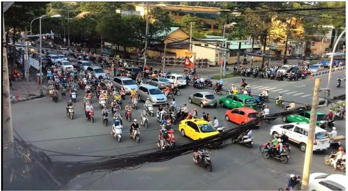
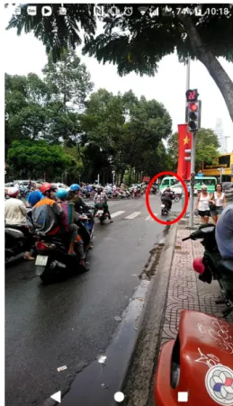
The capacity of a traffic stream is one of the most significant parts of traffic performance analysis. Particularly, capacity analysis of signalised intersections has been studied in developed countries where the primary transportation mode is the private car usage. In some developing countries, however, there are much distinctive traffic flow characteristics in contrast with those in developed countries such as 80% of the traffic composition being motorcycles, leading to the term ‘Motorcycle Dependent City (MDC)’ (Figure 1-1). Moreover, motorcycle driving behaviour in MDCs is entirely different from four-wheeled vehicle driving behaviour in car-dependent cities. Therefore, we cannot use models defined for car traffic in developed countries to analyse performances of motorcycle traffic and to evaluate the capacities of signalised intersections in developing countries such as Vietnam.

Figure 1-1: Traffic Operation at a Signalised Intersection in MDCs Note. Own Picture

This research focuses on proposing suitable models which can explain the specific characteristics of traffic streams in MDCs and the intersection capacities in different traffic situations.

1.2

The Concept of Motorcycle Dependent Cities

The term ‘Motorcycle Dependent City (MDC)’ has been presented by Khuat (2006). The motorcycle dependence is defined by three groups of indicators: vehicle ownership, availability of alternatives to motorcycle and car, and use of the motorcycle. The rating system (high, medium, low) of grading motorcycle dependence is shown in Table 1-1.

2

Table 1-1: Indicators of the Motorcycle Dependence

Indicators Level

Low Medium High

Main Criteria Sub-criteria Measurements Value Grade

Point Value Grade Point Value Grade Point Vehicle Ownership Motorcycle ownership MCs/1000 inhabitants < 150 1 150-350 2 > 350 3 Private car ownership PCs/1000 inhabitants < 150 3 150-350 2 > 350 1 Availability of Alternatives to Motorcycle and Car Bus transport availability Buses/ 1000 inhabitants < 1 3 1- 2 2 > 2 1 Bicycle availability Bicycles / 1000 inhabitants <150 1 150-350 2 >350 3 Use of Motorcycle Motorcycle share in the traffic flow % of MCs in the traffic flow (in vehicle unit) <30% 1 30 – 50% 2 > 50% 3 Modal split of motorcycle % of trips by motorcycles <20% 1 20 -40% 2 > 40% 3 Modal split of public transport % of trips by public transport < 20% 3 20-40% 2 > 40% 1 Modal split of

private car % of trips by cars < 20% 3 20- 40% 2 > 40% 1 Modal split of non-motorised traffic % of trips by non-motorised traffic < 20% 3 20 – 40% 2 > 40% 1 Note. Adapted from Khuat (2006), p. 36.

In Table 1-1, the rate of motorcycle dependence is defined based on the grade points average (GPA). The motorcycle dependence is ‘high’ if the GPA is higher than 2.5; the ‘medium’ motorcycle dependence is rated for the GPA that falls in-between 2.0 and 2.5, and the ‘low’ motorcycle dependence is defined for the GPA lower than 2.0 (Khuat, 2006).

Even though the motorcycle dependence is defined as a high level when the motorcycle share is higher than 50% in Table 1-1, the observed data in this study show that the real motorcycle share in the mixed flow at any signalised intersection in the urban area is always higher than 70%. Thus, the traffic flow is considered as motorcycle dependent flow when the motorcycle share is higher than 50%, and the percentage of other four-wheeled vehicles are lower than 50%.

1.3

Research Questions

The primary mission of this thesis is to establish a proper capacity calculation procedure for signalised intersections within MDCs. To do so, issues should be investigated such as the traffic flow characteristics, the affecting factors for the capacity calculation procedure, the performance of a traffic signal, and the specific driving behaviour of motorcyclists. These issues have been brought into focus using the following research questions.

Research Question 1:

What is the state-of-the-art in signalised intersection capacity analysis?

Research Question 2:

3

Research Question 3:

What factors affect the capacity and the saturation flow rate in MDCs?

Research Question 4:

How could the capacity model be built up?

Research Question 5:

How could the recommended capacity model be applied in MDCs?

1.4

Goal and Objectives

The major goal of this study is to find out a measure that analyses the capacity of each stream at a signalised intersection and overall intersection capacity in MDCs. This goal can be divided into objectives as follows:

1.5

Scope of Work

The research area of this study is limited to the concept of MDCs in which motorcycle occupies a high share in traffic composition. Therefore, this study is conducted only within the framework of traffic characteristics under the specific traffic conditions in MDCs.

The intersection approach capacity is the primary purpose of this study. Thus, the approach width should remain the same. The approach width with a short left-turning lane or right-turning lane would not be considered in this thesis.

Most of the signal programs in this study are two-phase signal programs. Therefore, this study focuses on signalised intersection under the condition of the two-phase signal program.

Field observation are solely conducted in one place, Ho Chi Minh City, where the motorcycle dependence reaches extreme share in the traffic composition.

1.6

Structure of the Study

The beginning point for the research is a literature review on capacity calculation methods and affecting factors on the capacity of signalised intersections (Chapter 2). The chapter starts with a basic capacity calculation equation for a signalised intersection and introduction of some factors affecting the capacity and the saturation flow. The next section is the state-of-the-art of capacity analysis. Several capacity methods and capacity manuals in selected countries are introduced. Capacity models related to MDC condition from the previous studies are also be mentioned.

In Chapter 3, the specific traffic characteristics such as the vehicle characteristics, the volume characteristics, the speed characteristics, the lane use distribution characteristics, the signal programs, and the driver behaviours are analysed to understand the traffic stream performance at signalised intersections in MDCs. The vehicle characteristics refer to the diversity of vehicle types and vehicle dimensions. The volume characteristics, emphasise the extreme motorcycle rate in the traffic composition. Then, the speed characteristics point out how flows operate in different traffic situations. The lane use distribution characteristics show how lanes are assigned to vehicle types. After that, the

• Finding factors that affect the capacity of signalised intersections significantly. • Developing a suitable capacity calculation method.

4

signal programs which are being applied in MDCs are also introduced to analyse how they influence the intersection capacity. Finally, the specific behaviours of drivers are mentioned as unique affecting factors to the intersection capacity.

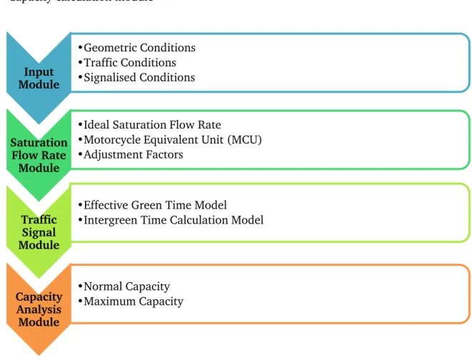
In Chapter 4, a capacity model structure and a capacity calculation procedure are developed. This model starts with introducing modules that create the whole capacity model. The input module includes input data needed for the capacity calculation. The saturation flow rate module shows the method and calculation steps for the saturation flow rate of each approach at a signalised intersection. The traffic signal module refers to the effective green time and other traffic signal program elements. The capacity analysis module describes the difference in capacity calculation including normal capacity and maximum capacity.

After introducing the theory capacity model in Chapter 4, empirical data is gathered to apply the model and to serve for the calibration process (Chapter 5). The surveys are conducted at urban signalised intersections in Ho Chi Minh City, Vietnam. Video observations such as traffic volume, speed, timing period, and traffic composition are implemented. The calibration process provides the plausibility of the theoretical model and the complete capacity model in MDCs.

Chapter 6 presents the model application. In this chapter, a completed capacity model, and a detailed procedure are depicted as a capacity calculation guideline. The guideline format is organised based on both the calculation form in the German Highway Capacity Manual (FGSV, 2015) and the U.S. Highway Capacity Manual (TRB, 2010). In Chapter 7, a sample calculation is introduced, by applying the guideline in Chapter 6. A typical four-leg signalised intersection is selected to calculate the intersection capacity by using the suggested guideline.

5

2

Capacity Calculation

2.1

Introduction

The comprehensive literature review is performed in this chapter. The primary method for the capacity analysis of signalised intersections is discussed. This part also highlights the importance of the saturation flow rate in the capacity analysis. Section 2.2 refers to the capacity and saturation flow rate models with some influencing factors. Section 2.3 is the state-of-the-art of capacity analysis. From this section, several methods and manuals in car traffic-based condition such as German Highway Capacity Manual (HBS) (FGSV, 2015), American Highway Capacity Manual (HCM) (TRB 2010), Indonesia Highway Capacity Manual 1997 (IHCM 1997), Malaysia Highway Capacity Manual 2011 (MHCM 2011), and the Manual on Traffic Signal Control in 2006 (JSTE 2006) are introduced. Besides, some models from research projects in MDCs are mentioned to show different traffic situations between these cities and others. Section 2.4 and section 2.5 refer to the effective green time and the intergreen time calculation which are the primary part of the comprehensive capacity model. Some conclusions from the literature are abridged in section 2.6 to conclude essential issues for the next steps.

2.2

Capacity and Saturation Flow Rate at Signalised Intersections

The capacity of signalised intersections is based on the lane group capacity and its relationship to demand flow rate. TRB (2010) defines capacity as ‘the maximum number of vehicles that can reasonably be expected to pass through the intersection under prevailing traffic, roadway, and signalisation conditions during a 15-min period’. The capacity of a lane or a lane group may be stated as shown in Equation 2-1: g C

t

C

S

t

=



where 𝐶 = Lane capacity [veh/h]

𝑡𝑔 = Effective green time [s]

𝑡𝐶 = Cycle length [s]

𝑆 = Saturation flow rate [veh/h]

The saturation flow rate is defined as the maximum number of vehicles which pass through an intersection approach when the signal is green, and enough vehicles exist to achieve a continuous flow to the end of the queue. The unit of the saturation flow rate is ‘vehicle per effective-green-hour’. The saturation flow rate is calculated by adjusting the base saturation flow rate to the specific conditions present on the subject intersection approach through adjustment factors. Equation 2-2 is used to compute the adjusted saturation flow rate per lane for the subject lane group:

0 x

S =S  f (2-2)

where 𝑆 = Lane saturation flow rate [veh/h]

𝑆0 = Base saturation flow rate [s]

𝑓𝑥 = Adjustment factors [s]

The adjustment factors may vary across countries depending on their specific traffic conditions. Table 2-1 shows the adjustment factors for the saturation flow rate of a signalised intersection. These factors do not influence the saturation flow or the capacity independently but in the way of combining with each other.

6

Table 2-1: Adjustment Factors for Saturation Flow Rate at Signalised Intersections

Application Field HBS 2015 HCM 2010 JSTE 2006 IHCM 1997 MHCM 2006 Road conditions Lane width ✓ ✓ ✓ ✓ ✓ Grade ✓ ✓ ✓ ✓ ✓

Intersection geometry (radius of turn, angle, visibility, etc.)

✓ ✓ ✓ ✓ ✓

Traffic conditions

Vehicle type (heavy vehicles, motorcycles, etc.) ✓ ✓ ✓ ✓ ✓

Parking ✓ ✓ ✓ Bus stop ✓ ✓ Lane utilisation ✓ Pedestrians crossing ✓ ✓ ✓ ✓ Control conditions Turning movements ✓ ✓ ✓ ✓ Opposing movements ✓ ✓ ✓

Duration of green time ✓ ✓ ✓

Behaviour conditions

Motorcyclist behaviour ✓

Regional characteristics (urban, rural) ✓ ✓ ✓

Note. Factors are retrieved from FGSV (2015), TRB (2010), JSTE (2006), IHCM (1997), and MHCM (2006)

Road Conditions

Lane Width

Lane width is the most influential parameter for the saturation flow rate. Apparently, when the lane width rises, the saturation flow rate also increases in correspondence and vice versa. The lane width adjustment factor accounts for the negative impact of narrow lanes on the saturation flow rate and allows for an increased flow rate on wide lanes (TRB, 2010). When determining the saturation flow rate, the lane width adjustment factors reflect the effect of lane width on free-flow speed.

Typically, a standard lane width value will be determined with an influenced degree by 1 to the saturation flow rate. The saturation flow rate will rise or goes down respectively depending on increasing or decreasing of the lane width. The standard lane width varies among different specifications (Table 2-2).

Table 2-2: Standard Lane Width

Specification HBS 2015 HCM 2010 JSTE 2006 IHCM 1997 MHCM 2006

Standard Lane Width (m) 3 3.6 3 3 3.6

Note. Adapted from FGSV (2015), TRB (2010), JSTE (2006), IHCM (1997), and MHCM (2006)

Grade

The vertical grade factor has also the primary effect on vehicle performance. The vertical grade at an intersection increases start-up lost time and diminishes vehicle running speed because it influences acceleration and deceleration of vehicles. As a result, the saturation flow rate is reduced by the vertical grade. Besides that, the effect of the grade is more significant during winter or wet conditions.

7

Intersection Geometry

The geometric characteristics of an intersection are effective factors for the saturation flow rate and the performance when loaded with traffic. The interaction of lane width with other geometric elements, shoulder width, curb, and media, also affect the traffic performance. Apparently, the saturation flow rate and speed at a given flow have higher values for wider shoulder conditions. The saturation flow rate is reduced if there is a fixed obstruction close to the edge of the carriageway, whether the road has a curb or a shoulder. Presence or absence of median also affects the saturation flow, and well-designed median contributes to increasing the saturation flow rate.

Traffic Conditions

Vehicle Type

Traffic flows comprise various kinds of vehicles such as heavy vehicles, small-sized commercial vehicles, cars, vehicles with small engines, motorcycles, bicycles and so on. The proportion of these vehicles has an influence on the lane or lane group’s saturation flow rate. In car traffic-based condition, the ideal saturation flow rates are given to passenger cars and the impact of other vehicles is considered usually based on passenger car units.

Heavy vehicles are considered as the most influential vehicle type for saturation flow rate. TRB (2000) defined heavy vehicles as those with over four tires touching the pavement. The heavy vehicles require additional spaces while operating compared with passenger cars. Thus, heavy vehicles in the traffic flow reduce the saturation flow rate.

Parking

Parking factor is important for the frictional effect of a parking lane on flow in an adjacent lane group and for the occasional blocking of an adjacent lane by vehicles moving into and out of parking spaces (TRB, 2010). In addition, on-street parking reduces the effective approach width, narrows down the queuing and discharge space, and influences the saturation flow rate of that approach.

Bus Blockage

Bus blockage factor represents the impacts of activities of buses at the stop station for picking up passengers at a near-side or far-side bus stop within the stop line. Usually, the impact of bus stops on saturation flow is significant only when buses regularly block traffic lanes during the green interval or its portion. This factor should be considered when the total expected waiting time occupies a considerable proportion of the green interval.

Lane Utilisation

The demand flow rate usually varies on the lanes in a lane group and reduce the saturation flow rate of that lane group. Thus, the lane utilisation factor is introduced to explains the unequal distribution of traffic among lanes in a lane group with more than one lane (TRB, 2000). In car traffic-based cities, this factor may adjust the base saturation flow rate. In motorcycle dependent cities, however, this factor cannot be applied because motorcycles do not operate under lane discipline rule.

8

Pedestrian Crossing

Pedestrian crossing factor only affects left-turning movements in case of permissive left turns with pedestrians. If the pedestrian flow rate operates during a part of the green interval when left-turning movements must wait for the opposing queue to discharge. It may cause a significant underestimation of the left-turning saturation flow rate.

Right-turning flows are affected by pedestrians using parallel crosswalks during the same phase. In areas of higher pedestrian activity, some pedestrians walking on the sidewalks may suddenly enter the crosswalks, and drivers, therefore, proceed cautiously. This movement causes reduce the saturation flow rate of the right-turning lane. On the other hand, where a few pedestrians are presented, or sidewalks are not provided, pedestrians have virtually no effect on the right-turning saturation flow rate (Teply et al., 2008).

Control Conditions

The control conditions are represented by the phasing structure as the composition of individual phases and specific green intervals. These conditions have a significant impact on the saturation flow (Teply, 1988).

Turning Movements

Turning effects are related to the effect of geometry. The right-turning adjustment factor depends on many variables such as exclusive lane or shared lane and proportion of right-turning movements in the shared lanes. In case of the existence of right-turning lanes with a protected right-turning phase, the saturation flow rate of right-turning lanes is influenced just by road conditions. In case of the existence of right-turning lanes without a protected right-turning phase, the saturation flow rate of right-turning lanes decreases because of the interactions between turning movements and crossing pedestrians.

The left-turning adjustment factor is based on the variables similar to those for the right-turning adjustment factor, including exclusive or shared lanes, left-turning proportion, and opposing flow rate. Exclusive left-turning lanes should be given to left-turning traffic in principle. In car traffic dependent condition, sometimes through and left-turning movements share the same lane because of various conditions. Lanes shared by through and left-turning movements are considered as through lanes and their saturation flow rates are adjusted for left-turning movements because through traffic are disturbed by left-turning traffic.

Opposing Movements

Left-turning movements which traverse stop lines during an unprotected left-turning phase is influenced by the opposing through-traffic. During the same phase, left-turning movements must find time gaps during which they can safely complete their turning movements in the opposing through-traffic. In car traffic-based cities, vehicles can only pass the intersection through the unsaturated opposing flow. In motorcycle traffic, real observations show that motorcycles even can pass the intersection through the saturated opposing flow under some certain conditions which can be explained in the next chapters.

9

Duration of Green Time

The first 5-7 vehicles crossing the stop line during the initial period of a green interval usually require longer headways than subsequent parts (Teply et al., 2008). As a result, the maximum saturation flow is not fully developed in this situation. Moreover, some drivers in the long queues become less attentive and do not move immediately after the preceding vehicle where long green intervals with fully a saturated flow. Therefore, their headways are longer than the minimum saturation flow headway during the steady flow portion of the green interval.

Behaviour conditions

Motorcyclist Behaviour

Motorcycles have the capability to move through queues in congested areas. Motorcycles are capable of zigzag manoeuvres and non-lane-based movements. They likely change their positions to more convenient areas to move forward or turn right/left. Inside the intersections, motorcycles tend to make groups to cross the intersection makes drivers feel safer and more confident (Huynh, Boltze, Vu, 2013). Obviously, motorcyclist behaviour through its unique characteristics was proven to affect the saturation flow rate.

Regional Characteristics

The area type has to be taken into account for the relative inefficiency of intersections in business districts in comparison with those in other locations (TRB, 2000). The saturation flow rate of signalised intersections in central business district (CBD) is lower than the one in other areas because there are many traffic activities operate in CBD area such as parking movements, taxi and bus operations, and high pedestrian activities.

2.3

State of the Art in Capacity and Saturation Flow Rate at Signalised Intersections

The capacity analysis is a set of procedures used to estimate the traffic carrying capacity of transportation facilities over a range of defined operational conditions. Different applied procedures through out countries have slightly different approaches to conducting capacity analysis. These procedures have been developed according to the respective countries’ traffic behaviour. Therefore, to come up with the best procedure for the country, local studies must be conducted.

The Intersection capacity is calculated based on the saturation flow rate and the signal timing parts, such as the effective green time and the cycle time. The saturation flow rate is computed by multiplying the base saturation flow rate under standard condition by affecting factors.

Capacity Analysis in Car Traffic-Based Cities

Webster and Cobbe

Webster and Cobbe (1966) defined the saturation flow rate as the flow, which would be obtained If there was a continuous queue of vehicles and they were given a 100 per cent green time’. It is expressed in vehicles per hour of green (vphg).

10

Figure 2-1: The Flow of Traffic during the Green Period from a Saturated Approach Note. Adapted from Webster amd Cobbe (1966)

The concept ‘effective green’ period is shown in Figure 2-1 to have the constant value of the saturation rate. It means that the curve in Figure 2-1 is replaced by an equal area rectangle. Therefore, the effective green time is equal to the green time minus the start-up lost time, then plus a part of the amber time.

The unit of pcu/h (passenger car unit per hour) is used to express the saturation flow rate. The saturation flow rate is affected by approach width, gradients of approach, traffic composition (each vehicle type is equivalent to some private cars respect its road-capacity requirements), right-turning traffic, left-turning traffic, pedestrians, parked vehicles, and site characteristics.

Table 2-3: The Effect of Lane Width on Saturation Flow

Lane Width (m) 3.05 3.35 3.66 3.96 4.27 4.57 4.87 5.18

Saturation Flow (pcu/h) 1,850 1,875 1,900 1,950 2,075 2,250 2,475 2,700 Note. Adapted from Webster and Cobe (1966)

G

ermany

According to the Germany Highway Capacity Manual (FGSV, 2015), the basic saturation flow rate 𝑆0 is 2,000 pcu/(h*ln). A basic saturation headway 𝑡𝐻,0=1.8 s/(veh*ln) is used for the base condition. In the manual, heavy vehicles influence the value of saturation flow rate significantly and it is considered as a separated factor. The saturation flow rate has an inverse ratio to this factor. Moreover, some affecting factors are also computed such as lane width, turning radius, and grade. Considering external conditions, the saturation flow rate is computed as:

,0 1 2

3, 600

3, 600

S

t

t

f

f

f

=

=



 

Where 𝑆 = Adjusted saturation flow rate [veh/(h*ln)]

𝑡𝐻 = Adjusted saturation headway [s/(veh*ln)]

11 𝑓𝐻𝑉 = Adjustment factor for heavy vehicles in the traffic stream [-]

𝑓1 = Max (𝑓𝑏, 𝑓𝑅, 𝑓𝑆) [-]

𝑓2 = Min (1, 𝑓𝑆) [-]

𝑓𝑏 = Adjustment factor for lane width [-]

𝑓𝑅 = Adjustment factor for turning radius [-]

𝑓𝑆 = Adjustment factor for approach grade [-]

United States of America

The Highway Capacity Manual (TRB, 2010) is developed as a comprehensive revision of the previous manuals in the U.S. As explained in previous sections, the first step taken in the capacity analysis is to determine the saturation flow for the single lanes in the intersection. TRB (2010), a saturation flow rate for each lane group is calculated according to Equation2-4 where the ideal saturation flow for this method is 1,900 pc/(h*ln). The saturation flow rate is the flow in vehicles per hour that can be accommodated by the lane group assuming that the green phase is displayed 100 per cent of the time (i.e., g/C= 1.0).

𝑆 = 𝑆0𝑓𝑤𝑓𝐻𝑉𝑓𝑔𝑓𝑝𝑓𝑏𝑏𝑓𝑎𝑓𝐿𝑈𝑓𝐿𝑇𝑓𝑅𝑇𝑓𝐿𝑝𝑏𝑓𝑅𝑝𝑏 (2-4)

Where 𝑆 = Saturation flow rate for subject lane group, expressed as a total for all lanes in lane group

[veh/h]

𝑆0 = Base saturation flow rate per lane S0=1,900 pcu/(h*ln) [pcu/(h*ln)]

𝑓𝑤 = Adjustment factor for lane width [-]

𝑓𝐻𝑉 = Adjustment factor for heavy vehicle in the traffic stream [-]

𝑓𝑔 = Adjustment factor for approach grade [-]

𝑓𝑝 = Adjustment factor for existence of a parking lane and parking activity adjacent to lane group

[-]

𝑓𝑏𝑏 = Adjustment factor for blocking effect of local buses that stop within intersection area

[-]

𝑓𝑎 = Adjustment factor for area type [-]

𝑓𝐿𝑈 = Adjustment factor for lane utilisation [-]

𝑓𝐿𝑇 = Adjustment factor for left turns in a lane group [-]

𝑓𝑅𝑇 = Adjustment factor for right turns in a lane group [-]

𝑓𝐿𝑝𝑏 = Pedestrian adjustment factor for left-turning groups [-]

𝑓𝑅𝑝𝑏 = Pedestrian-bicycle adjustment factor for right-turning groups [-]

Japan

In Japan, the Manual on Traffic Signal Control (JSTE, 2006) determined the saturation flow rate based on the ideal saturation flow rate multiplying several adjustment factors.

    

a B w G T RT LT

S = S × × × × × (2-5)

Where 𝑆𝑎 = Saturation flow rate for subject lane group, expressed as a total for all lanes in lane group

[veh/h]

𝑆𝐵 = Ideal saturation flow rate [pcu/(h*l)]

𝛼𝑤 = Adjustment factor for lane width [-]

𝛼𝐺 = Adjustment factor for vertical grade [-]

𝛼𝑇 = Adjustment factor for heavy vehicles [-]

𝛼𝑅𝑇 = Adjustment factor for right-turning movements [-]

12

The ideal saturation flow rate means the departure rate from each vehicle queue during an hour of green time where road and traffic conditions are ideal. According to the actual measurement, the saturation flow rate of through lane is from 1,800 veh/h to 2,200 veh/h, left-turning lane is from 1,660 veh/h to 1,840 veh/h, and right-turning lanes is from 1,870 veh/h to 2,120 veh/h.

Indonesia

According to the Indonesia Highway Capacity Manual (IHCM, 1997), the saturation flow 𝑆 can be expressed as a product between a base saturation flow 𝑆0 for a set of standard conditions, and correction factors F for deviation of the actual conditions from a set of pre-determined (ideal) conditions. The equation of saturation flow is given as:

𝑆 = 𝑆0× 𝐹𝐶𝑆× 𝐹𝑆𝑃× 𝐹𝐺× 𝐹𝑃× 𝐹𝑅𝑇× 𝐹𝐿𝑇

The base saturation flow 𝑆 is determined as a function of an approach width 𝑊𝑒 and the flow of right-turning traffic in the own approach and in the opposing approach since the influence of these factors is non-linear. Corrections are then made for actual conditions regarding city size, side friction, gradient, and parking as in formula 2-8 below:

𝑆0= 600 × 𝑊𝑒 (2-7)

Where 𝑆0 = Base saturation flow rate per lane 𝑆0= 1,900 pcu/(h*ln) [pcu/(h*ln)]

𝑊𝑒 = Effective approach width [m]

𝐹𝐶𝑆 = The city size correction factor [-]

𝐹𝑆𝑃 = The side friction correction factor [-]

𝐹𝐺 = The gradient correction factor [-]

𝐹𝑃 = The parking correction factor [-]

𝐹𝑅𝑇 = The right turn correction factor [-]

𝐹𝐿𝑇 = The left turn correction factor [-]

Malaysia

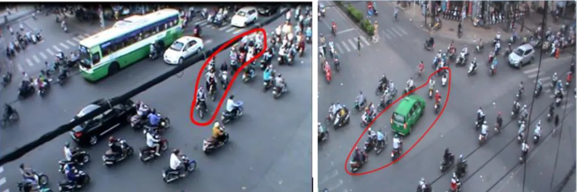
The effect of motorcycle traffic on the saturation flow rate is considered for the capacity estimation based on the Malaysia Highway Capacity Manual (MHCM, 2011). Motorcyclists’ behaviour at the intersection can be regrouped into two categories namely motorcycles outside flow and motorcycles within the flow. Motorcycles outside flow are motorcycles that do not follow the first-in-first-out rule. This group includes motorcycles in front of the stop line and motorcycles beside other vehicles. Motorcycles inside flow are motorcycles that follow the first-in-first-out rule implying that they either travel in front of or behind other vehicles within a traffic stream. Both categories affect the value of saturation flow and consecutively affects the capacity of the road (Ministry of Works Malaysia, 2011). Figure 2-3 shows the distribution of motorcycles inside flow and motorcycles outside flow which are common in Malaysia.

13

Figure 2-2: The Distribution of Motorcycles inside Flow and Motorcycles outside Flow Note. Retrieved from Vien et al. (2008), p.03

The saturation flow rate 𝑆 can be expressed as a product between a base saturation flow rate 𝑆0 for a set of standard conditions, and correction factors 𝑓 for deviation of the actual conditions from a set of pre-determined (ideal) conditions. The equation of saturation flow is shown by:

0 1 w g a c S S f f f f   =   _{  }   (2-8)

Where 𝑆0 = Base saturation flow rate per lane, 1930 pcu/(h*ln) [pcu/(h*ln)]

𝑓𝑤 = The lane width factor [m]

𝑓𝑔 = The grade factor [-]

𝑓𝑎 = Type of area factor [-]

𝑓𝑐 = The vehicle composition factor [-]

Capacity Analysis in Motorcycle Dependent Cities

Chu

’s

Method

Chu and Sano (2003) proposed saturation flow rate models in which the effects of the motorcycle both heterogeneous traffic and car traffic at signalised intersections in developing countries. The data was collected in Bangkok, Thailand, and Hanoi, Vietnam by using video method, manual counting and measurement. A comparison of two traffic situations was conducted to get suitable results. In Hanoi, four intersections were surveyed at the morning peak period (7 am- 9 am) and the afternoon peak period (4 pm–6 pm). The study approaches were similar characteristics. They were fixed time signalised control and have 3.5m-5m lane widths. The proportion of motorcycles was an average of 90% of all transportation modes.

In Bangkok, the traffic data was collected during peak period from 11 am to 1 pm and 4 pm to 6 pm. The lane widths were varied from 3.2 m to 5 m, and the motorcycle shared average 20% of total traffic flow.

14

Traffic compositions were classified into three groups: group 1 includes motorcycle, mopeds, and scooters; group 2 includes passenger cars, vans and taxis; group 3 includes buses. The different saturated green times from 5 s to 45 s were recorded to estimate the equivalent factor of the motorcycles into passenger car units, the average saturation headway, and the saturation flow rate. Chu assumed that the saturated green time is a function of the number of vehicles passing the stop line during the green time in which the relationship between dependent variables is linear.

𝑡 = 𝑎1. 𝑛1+ 𝑎2⋅ 𝑛2+ 𝑎3. 𝑛3 (2-9)

where 𝑡 = Saturated green time [s]

𝑎1, 𝑎2, 𝑎3 = Coefficients of motorcycle, private car, and bus [s/veh]

𝑛1, 𝑛2, 𝑛3 = The number of vehicles in each group crossing the approach [veh] Chu converted all the vehicles passing the stop line to passenger car equivalent during each five-second interval. Then, in every five five-seconds in green time, if more than three PCUs passing through the stop line, that time is considered as saturated green time and the traffic is saturated.

Table 2-4: Passenger Car Unit (PCU)

Vehicle PCU

Motorcycle, moped, scooter 0.25

Passenger car, van, taxi 1.00

Bus 2.00

Note. Adapted from Chu (2003), p.1215

The saturated green time is divided by the total number of vehicles (PCU) to the average headway. The formula is shown below:

1 1 2 2 3 3

t

H

n p



n



p

+ 

n

p

=

+

where 𝐻 = Average headway [s/pcu]

𝑝1; 𝑝2; 𝑝3 = The PCU values for motorcycles, passenger cars, and buses respectively

[-]

𝑛1; 𝑛2; 𝑛3 = The number of vehicles in each group crossing the [veh] From the average saturation headway H, the saturation flow rate is then determined by the

Formula: 3600

H [pcu/h].

After regression analyses from the collected data, Chu achieved the results as: In Hanoi: 𝑡 = 0.207 ⋅ 𝑛1+ 0.85 ⋅ 𝑛2+ 1.918 ⋅ 𝑛3 with R2=0.99

In Bangkok: 𝑡 = 0.281 ⋅ 𝑛1+ 1.603 ⋅ 𝑛2+ 3.487 ⋅ 𝑛3 with R2=0.99 Table 2-5: Passenger Car Unit (PCU) for Other Vehicles

City Motorcycle Car, van, taxi Bus

Ha Noi 0.24 1.00 2.26

Bangkok 0.18 1.00 2.18

15

Table 2-6: Estimated Saturation Flow Rate

City Average Headway Statistics Saturation Flow Rate (PCU/egh) Mean [s] Standard Deviation [s]

Ha Noi 0.88 0.11 4,092

Bangkok 1.6 0.12 2,253

Note. Adapted from Chu (2003), p.1216

The regression model considers the influence of two main factors (lane width, number of motorcycles) on saturation flow rate S (pcu/h).

(

)

1965 105

- 3.5

0.12

S

=

+



w

+



mc

Where 𝑆 = Saturation flow rate [pcu/h]

𝑤 = Lane width [m]

𝑚𝑐 = Number of motorcycles passing the stop line in one hour. [veh/h]

Nguyen

‘

s Method

The second research is conducted by Nguyen et al. (2007) about the saturation flow in traffic dominated by motorcycles. Authors proposed a methodology to study the variation of saturation flow and vehicle equivalence factorssimultaneously, and the motorcycle was selected as the basis to study other categories of the vehicle as well as the whole traffic flow.

The regression analysis was also used for this study. Twelve approaches which have 3.9 m -13 m width were collected in Hanoi, Vietnam. The traffic compostion included private cars, light van, minibus, bus, coach, motorcycle, and bicycle. The motorcycle proportion was varying from 80% to 95%.

The Road Note 34 method (Webster, 1963) was applied in this study. In this method, a 6 s period was selected normally. However, Nguyen (2007) decided to count in every consecutive 4 seconds in case traffic dominated by motorcycles. For every 4 s period, vehicles were classified according to turning movements (straight, left turn and right turn) and vehicle categories.

At a starting point, they assumed that 𝑆 is the motorcycle saturation flow rate during a specific period T (for example, 4 s). If the traffic flow includes 𝑁𝑚𝑐 motorcycles 𝑁𝑐passenger cars, then the saturation flow rate is expressed as.

𝑆 = 𝑁𝑚𝑐+ 𝑀𝐶𝑈𝑐⋅ 𝑁𝑐 (2-12)

where 𝑆 = Saturation flow rate [MCU/4s]

𝑁𝑚𝑐; 𝑁𝑐 = The numbers of motorcycles and passenger car crossing the stop line within 4 s periods

[veh/4s]

𝑀𝐶𝑈𝑐 = Equivalent factor of one passenger car into motorcycles [MCU]

It is assumed that 𝑀𝐶𝑈𝑐 varies depending on the number of cars in the stream, the variation would be linearly related to the number of cars in the stream, as presented in Equation 2-13:

𝑀𝐶𝑈𝑐 = 𝑚 + 𝑛 ⋅ 𝑁𝑐 (2-13)

By using both Equations 2-12 and 2-13, a multiple linear regression equation with explanatory variables 𝑁𝑐 and 𝑁𝑐2 was created.

16

𝑁𝑚𝑐 = 𝑆 − 𝑚 ⋅ 𝑁𝑐− 𝑛 ⋅ 𝑁𝑐2 (2-14)

A model to estimate the saturation flow rate is shown in the equation below:

𝑁𝑚𝑐 = 𝑎 + 𝑏 ⋅ (𝑊 − 3.5) + 𝑐 ⋅ 𝑃𝑟𝑡/𝑅𝑟𝑡+ 𝑑 ⋅ 𝑃𝑙𝑡/𝑅𝑙𝑡 (2-15)

where 𝑊 = Approach width [m]

𝑃𝑟𝑡; 𝑃𝑙𝑡 = Proportion of right-turning and left-turning motorcycles [-]

𝑅𝑟𝑡; 𝑅𝑙𝑡 = Right-turning and left-turning radius [m]

𝑎; 𝑏; 𝑐; 𝑑 = Coeffiecients [-]

By combining of Equation 2-14 and 2-15, an equation representing the relationship between 𝑁𝑚𝑐 and other factors can be written as in Equation 2-16:

𝑁𝑚𝑐 = 𝑎 + 𝑏 ⋅ (𝑊 − 3.5) + 𝑐 ⋅ 𝑃𝑟𝑡/𝑅𝑟𝑡+ 𝑑 ⋅ 𝑃𝑙𝑡/𝑅𝑙𝑡− 𝑚 ⋅ 𝑁𝑐− 𝑛 ⋅ 𝑁𝑐2+ 𝜀 (2-16) When traffic contains all types of vehicles, i.e. motorcycles, passenger cars, vans and buses and all

turning movements, i.e. straight, right turners and left turners, Equation 2-16 needs to be changed to reflect the effect of turning movements. Therefore, their effects are represented by three different factors as described in Equation 2-17.

2 2 2 1 1 2 2 3 3 2 2 2 1 1 2 2 3 3 2 2 2 1 1 2 2 3 3 ( 3.5) / / mc rt rt lt lt cst cst crt crt clt clt vst vst vrt vrt vlt vlt bst bst brt brt blt blt N a b W c P R d P R m N n N m N n N m N n N p N q N p N q N p N q N r N s N r N s N r N s N  = +  − +  +  −  −  −  −  −  −  −  −  −  −  −  −  −  −  −  −  −  −  + (2-17)

Where 𝑁𝑐𝑠𝑡; 𝑁𝑐𝑟𝑡; 𝑁𝑐𝑙𝑡 = The numbers of straight, right-turning, and left-turning cars

[veh/4s]

𝑁𝑣𝑠𝑡, 𝑁𝑣𝑟𝑡, 𝑁𝑣𝑙𝑡 = The numbers of straight, right-turning and left-turning vans,

[veh/4s]

𝑁𝑏𝑠𝑡, 𝑁𝑏𝑟𝑡, 𝑁𝑏𝑙𝑡 = The numbers of straight, right turning and left-turning buses

[veh/4s]

𝑚𝑖, 𝑛𝑖, 𝑝𝑖, 𝑞𝑖, 𝑟𝑖, 𝑠𝑖 = Coefficients [-]

The mixed traffic streams need to be converted to homogeneous flow before calculating proportions of vehicle stream. To do so, a pre-defined set of MCU values need to be known. However, MCU values are coefficients of regression models, their exact values can only be obtained after these regression models are calibrated. Hence an iteration approach was introduced to deal with the situation. MCU values for 4.0 for passenger cars, 8.0 for vans and minibuses and 10 for buses as used in Vietnam were used as the initial value. These were used to convert a mixed flow to an equivalent homogeneous stream, and proportions of turning motorcycles were computed. The models were run and revised MCU values were obtained. Then, these MCU values were used to recalculate the portions of right and left turners. The process was repeated until the differences of MCU values from two consecutive loops were smaller than 1%.