Repository and Information Exchange
Theses and Dissertations2017
Response Surface Methodology and Its
Application in Optimizing the Efficiency of
Organic Solar Cells
Rajab Suliman
South Dakota State University
Follow this and additional works at:http://openprairie.sdstate.edu/etd
Part of theStatistics and Probability Commons
This Dissertation - Open Access is brought to you for free and open access by Open PRAIRIE: Open Public Research Access Institutional Repository and Information Exchange. It has been accepted for inclusion in Theses and Dissertations by an authorized administrator of Open PRAIRIE: Open Public Research Access Institutional Repository and Information Exchange. For more information, please [email protected]. Recommended Citation
Suliman, Rajab, "Response Surface Methodology and Its Application in Optimizing the Efficiency of Organic Solar Cells" (2017).
Theses and Dissertations. 1734.
OPTIMIZING THE EFFICIENCY OF ORGANIC SOLAR CELLS
BY
RAJAB SULIMAN
A dissertation submitted in partial fulfillment of the requirements for the Doctor of Philosophy
Major in Computational Science and Statistics South Dakota State University
ACKNOWLEDGEMENTS
I would like to express my sincere gratitude to my advisor Dr. Gemechis D. Djira for accepting me as his advisee since November 2016. He has helped me to successfully bring my Ph.D. study to completion. In particular, he has helped me to develop
simultaneous inferences for stationary points in quadratic response models. I also worked with Dr. Yunpeng Pan for three years. I appreciate his guidance and support. I could not have imagined successfully completing of my Ph.D. study without their continuous support, motivation, patience, and enthusiasm, especially through difficult times, to achieve my long-sought goal. Dr. Pan also facilitated our collaboration with the
Department of Electrical Engineering and Computer Science. In this regard, I would also like to express my sincere thanks to Dr. Qiquan Qiao and Mr. Abu Farzan Mitul from Electrical Engineering and Computer Science Department for their assistance in
generating the data we used for the organic solar cell experiment. They have provided an excellent environment that will foster to carry on my future independent research.
I would also gratefully acknowledge Dr. Kurt Cogswell, Head of the Mathematics and Statistics Department, and Dr. Donald Vestal, graduate program coordinator in the Department of Mathematics and Statistics, for their support. I am also grateful to all of my Ph.D. advisory committee members including Dr. Gary Hatfield and Thomas Roe from the Department of Mathematics and Statistics, and my graduate school
representative Dr. Jane Mort from the College of Pharmacy. They provided me with constructive comments which greatly improved the quality of my dissertation.
My especially thanks goes to the Ministry of Higher Education, Libya, for
sponsoring my Ph.D. study abroad through Libyan North American Scholarship Program (LNASP). My research is also partially benefitted by the NSF CAREER
(ECCS-0950731) , and NASA EPSCoR (NNX13AD31A) grants used for the organic solar cell experiment. I also sincerely acknowledge all faculty members in the Department of Statistics at Misurata University for their encouragement. I am also indebted to Dr. Yasmina Faqih, and Dr. Hussain Kaiba who was a great mentor. I want to thank him post hum for his support.
Last but not least, my sincere thanks to my family, especially to my mother, wife, brothers, and son, for their love, sacrifices, and encouragement that helped me to
complete my research. Finally, I must say that in the journey of my life I am indebted to so many of my family members, friends, and well-wishers who have provided invaluable advice during uncertain and challenging times and helped me to keep my dream alive. I wish I could thank every individual person, but nevertheless, they are always in my heart.
TABLE OF CONTENTS
LIST OF FIGURES ... ix
LIST OF TABLES ... xii
ABSTRACT ... xiv
GENERAL INTRODUCTION ...1
INTRODUCTION TO RESPONSE SURFACE METHODOLOGY ...3
2.1 Introduction ...3
2.2 Overview and stages for RSM application ...3
2.3 Screening experiment...6
2.4 Empirical model building ...6
2.5 Encoding of input variable levels ...12
2.6 First-order model ...12
2.6.1 Two-level factorial designs ...12
2.6.2 Two-level fractional factorial designs ...13
2.7 Blocking in response surface designs ...14
2.8 Steepest ascent ...16
2.9 A second-order experimental design ...21
2.9.1 Full 3K factorial designs ...21
2.9.2 Box–Behnken designs (BBD) ...22
2.9.4 Doehlert design ...25
2.10 Lack-of-fit test ...27
2.11 Variance dispersion graph...29
2.12 The Common design properties ...32
2.12.1 Orthogonality ...32
2.12.2 Rotatability ...32
2.12.2.1 Design moment matrix ...33
2.12.2.2 Rotatable conditions for first-order design ...35
2.12.2.3 Rotatability conditions for a second-order design ...36
2.12.2.4 Rotatability of the CCD ...37
2.13 Uniform precision ...38
MODELING OF ORGANIC SOLAR CELL USING RESPONSE SURFACE METHODOLOGY ...39
3.1 Introduction and background ...40
3.1 Materials, device fabrication and characterization ...44
3.1.1 Materials ...44
3.1.2 Single-junction device fabrication ...45
3.1.3 Current density – voltage (J-V) characterization ...45
3.2 Experimental design...46
3.3.1. Model fitting for first order design ...48
3.3.2 Moment matrix and rotatability conditions ...51
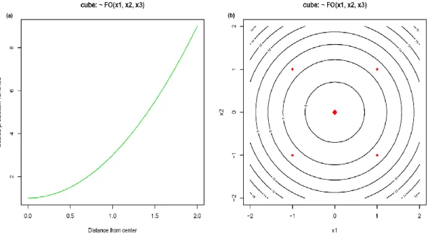
3.4. Augmenting further to fit a quadratic response surface ...52
3.5. Device structure ...57
3.6. Residual analysis for fitted quadratic model ...59
SIMULTANEOUS INFERENCE FOR THE LOCATION OF A STATIONARY POINT ... 62
4.1 Location of a stationary point ... 62
4.2 Confidence region for the location of a stationary point ... 66
4.2.1 Box and Hunter ... 67
4.2.2 Asymptotic confidence region for stationary point ... 69
4.3 Simultaneous confidence intervals for the coordinate of a stationary point ... 72
4.3.1 Bonferroni adjustment ... 74
4.3.2 Multiplicity adjustment based on equi-coordinate critical point ... 75
4.3.3 Bootstrap confidence intervals ... 76
4.4 Simulation study ... 77
4.5 Assessing the solar cell data using the bootstrap technique ... 80
4.6 Rising ridge in quadratic surfaces ... 83
4.6.1 Canonical analysis and confidence intervals for eigenvalues ... 84
COMBINATORIAL OPTIMATIZATION FOR DESIGN POINTS ... 94
5.1 Metaheuristics ... 94
5.2 Properties ... 96
5.3 Generalized and conditional inverse ... 98
5.3.1 Generalized inverse ... 98
5.4 The relative error with respect to the quadratic fitted model ... 101
RECENT DEVELOPMENT OF RESPONSE SURFACE METHODOLOGY ... 113
6.1 Multivariate response optimization... 113
6.2 Robust parameter design ... 115
6.2.1 Taguchi’s approach ... 116
6.3 Generalized linear models... 117
6.3.1 Local optimum designs ... 118
6.3.2 Sequential designs ... 118
6.3.3 Robust design technique ... 118
DISCUSSION AND CONCLUSION ... 120
7.1 Discussion and conclusions ... 120
7.2 Future research ... 122
APPENDIX A ... 131
APPENDIX B ... 135
LIST OF FIGURES
Figure 2.1. Flow chart of RSM………5
Figure 2.2. Full 32 factorial design (k = 2)………..7
Figure 2.3.(a) The expected efficiency (y) as a function of x1 and x3 and (b) A contour plot………...9
Figure 2.4. Response along the path of the steepest ascent.………..………...18
Figure 2.5. The three-level factorial design of (a) two factors and (b) three factors and (c) Box–Behnken design of three factors………23
Figure 2.6. CCD (a) two factors with α = 2 and (b) three factors with α = 1.68………...25
Figure 2.7. Doelhert design (a) two factors (b) three factors originated by the
two-plane………...26 8
Figure 2.8. VDG with three factor, five center point with α = 1.68 and α = 1.732……...30
Figure 2.9. VDG with k = 3, α = 1.68 and α = √2 (one to five center point).…………30
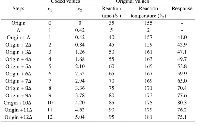
Figure 3.1. Full 23 factorial design with geometric view………..48
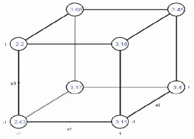
Figure 3.2. Variance function plots for a cube design: (a) Profile plot and (b) Contour plot……….49 Figure 3.3. Variance function plot for quadratic model: (a) Profile plot (b) Contour plot……….53 Figure 3.4. Contoure plot of the efficiency………57
Figure 3.5. Response surface plot for solar cell efficiency………58
Figure 3.6. Device layout of PDPP3T-PCBM single junction polymer solar cell………59
Figure 3.7. J-V Characteristic curves of (a) cube, (b) foldover, and (c) star functions….59
Figure 3.8.The residual analysis for fitted quadratic model………..61
Figure 3.9. The studentized and studentized residuals………..62
Figure 4.1. The surface and contour plots of the true regression function, β12= 0……...78
Figure 4.2 The surface and contour plots of the true regression function, β12 = 1……...79
Figure 4.3. A bivariate kernel density, β1 = 0, β2 = 0, and β12 = 0………..80
Figure 4.4. Bivariate kernel density estimate, estimated stationary point when β1= 0.4, β12 = 1.6, β12 = 0………...80 Figure 4.5. Bivariate kernel density estimate, estimated stationary point when β1= 0.4, β12 =1.6, β12 =1………....81 Figure 4.6. Bootstrap estimate for best combination of organic solar cell………82
Figure 4.7. Stationary point of organic solar cell, the design region is shown in red box.83
Figure 4.8. 90% Confidence regions and simultaneous confidence intervals…………...84
Figure 4.9. 95% Confidence regions and simultaneous confidence intervals…………...84
Figure 4.10. The individual approximate CI for the eigenvalues………..92
Figure 4.11. The individual approximate 95% Bonferroni CI for the eigenvalues…….94
Figure 5.2. The histogram of current solutions according to the relative error………...107
Figure 5.3. The current solution corresponding to the relative error………...107
Figure 5.4. The dynamic of default design points with respect to the second-order
model………112
LIST OF TABLES
Table 2.1. ANOVA for the first-order model………19
Table 2.2. Steepest ascent experiment………...19
Table 2.3. Data for quadratic model………..20
Table 2.4. ANOVA for quadratic model………...21
Table 2.5. Design matrix for three-level factorial design with two factors………...22
Table 2.6. Design matrix for Box–Behnken design with three factors………..23
Table 2.7. Design matrix for central composite design with three factors………25
Table 2.8. Doehlert matrices (a) with two variables, and (b) with three variables………26
Table 2.9. ANOVA table for lack-of-fit test………..28
Table 3.1. Design matrix of the CCD and the corresponding experimental results……..47
Table 3.2. The three factors and the levels utilized in the CCD………47
Table 3.3. The design matrix of 23 factorial design………..48
Table 3.4. The significance of the first-order effects according to the cube design……..50
Table 3.5. ANOVA table for lack-of-fit test……….56
Table 3.6. Observed values, Predicted values, Residuals, and other diagnostics………..60
Table 4.1. Estimates of the coverage probability (nominal: 1-α = 0.95)..……….79
Table 4.3. The approximate 95% confidence interval for estimated eigenvalues……….92
Table 4.4. The approximate 95% Bonferroni confidence interval for estimated
eigenvalues……...93 Table 5.1. The first permutation matrix (swap) generated within the blocks…………..103
Table 5.2. The last permutation matrix (swap) generated within the locks…………....104
Table 5.3.The relative error according to the 276 permutation matrices……….106
Table 5.4. The candidate trial solution (swap 44) with respect to the second-order
model………108 Table 5.5. The candidate trial solution (swap 183) with respect to the second-order
model………109 Table 5.6. The candidate trial solution (swap 184) with respect to the second-order
model………110 Table 5.7. The relative error according to each swap with their iteration………...111
ABSTRACT
RESPONSE SURFACE METHODOLOGY AND ITS APPLICATION IN OPTIMIZING THE EFFICIENCY OF ORGANIC SOLAR CELLS
RAJAB SULIMAN
2017
Response surface methodology (RSM) is a ubiquitous optimization approach used in a wide variety of scientific research studies. The philosophy behind a response surface method is to sequentially run relatively simple experiments or models in order to
optimize a response variable of interest. In other words, we run a small number of experiments sequentially that can provide a large amount of information upon augmentation. In this dissertation, the RSM technique is utilized in order to find the optimum fabrication condition of a polymer solar cell that maximizes the cell efficiency. The optimal device performance was achieved using 10.25 mg/ml polymer concentration, 0.42 polymer-fullerene ratio, and 1624 rpm of active layer spinning speed. The cell efficiency at the optimum stationary point was found to be 5.23% for the
Poly(diketopyrrolopyrrole-terthiophene) (PDPP3T)/PC60BM solar cells. Secondly, we
explored methods for constructing a confidence region for the stationary point in RSM. In particular, we developed methods for constructing simultaneous confidence intervals for the coordinates of a stationary point in a quadratic response surface model. The methods include Bonferroni adjustment, a plug-in approach based on the asymptotic distribution of maximum likelihood estimators, and bootstrapping. The simultaneous coverage probabilities of the proposed methods are assessed via simulation. The coverage
probabilities for the Bonferroni and plug-in approaches are pretty close to the nominal levels of 0.95 for large sample sizes. The metaheuristic method is also considered in order to search for an alternative solution to the design matrix that may be near to the optimal solution. Finally, we explored recent developments in RSM including
CHAPTER 1
GENERAL INTRODUCTION
It is important to any system to increase performance in order to increase the yield at low cost. One technique used for such a purpose is the so-called optimization.
Response surface methodology (RSM) is the most common optimization technique and it has been employed in many fields such as exploring chemical and biochemical processes. This technique is used to fit an empirical model to the experimental data. Usually, we consider several potential input variables that influence the system performance. Toward this aim, the lower order polynomial models are used in order to explore the system under study, and therefore, to describe an experimental design until the conditions is optimized. This dissertation focuses on various topics in RSM research. The specific objectives are:
i. Use RSM to find the optimum conditions that will optimize cell efficiency of
organic solar cell.
ii. Develop methods for constructing simultaneous confidence intervals for the
location of a stationary point.
iii. Utilize a metaheuristic approach in order to find an alternative optimum order of
the design points.
iv. Explore recent developments in RSM research.
In order to achieve these objectives, the dissertation is organized as follows.
In Chapter 2, general introduction to RSM and various RSM designs and their properties will be explored. In Chapter 3, organic solar cell data is analyzed using response surface methodology in order to optimize cell efficiency. These data have been
collected with the help of the Department of Electrical Engineering and Computer Science (EECS), South Dakota State University. The RSM technique will allow us to find the combination of input variables that will optimize a response variable of interest. In Chapter 4, methods for simultaneous inference concerning a stationary point of a quadratic response surface model are discussed. Three methods for constructing
simultaneous confidence intervals for the coordinates of a stationary point are developed. The coverage probabilities of these methods, namely, Bonferroni simultaneous
confidence intervals, plug-in method (based on an equi-coordinate critical point of a multivariate normal distribution), and the bootstrap technique are assessed using simulation. Chapter 5 presents a metaheuristic search method popular in Operations Research. By this approach, one searches for an alternative order in the default design matrix associated with RSM. This approach consists of a random search and swapping
within three blocks (cube, foldover, and star) to find an alternative solution. Chapter 6
deals with recent and advanced RSM topics such as generalized linear models (e.g., when the dependent variable is a count or binary in nature) and multivariate RSM with regard to robustness. Finally, Chapter 7 is devoted to discussions, conclusions, and some future research.
CHAPTER 2
INTRODUCTION TO RESPONSE SURFACE METHODOLOGY
2.1 Introduction
An essential part of any business is improving the performance of its processes and increasing the yields of the systems without increasing the associated costs. This process is referred to as optimization. A specific variable change in the general application can be determined under optimum conditions while holding the other variables at a constant level. This is often referred to as a one variable technique. One main disadvantage of using this technique is that it will not contain the interaction effects between the variables and, additionally, it will not fully describe the effects of the
variables on the procedure. In order to solve these problems, optimization studies can be achieved using the technique of response surface methology (RSM).
The RSM process is a group of statistical and mathematical methods used in developing, and optimizing process, in which a response surface of interest is effected by several variables. RSM is a powerful technique which has important applications in the design of an experiment, the development and design of a new product, and in the optimization of existing products and process designs. It defines the effects of the important factors, alone or in combination with the involved processes [1].
2.2 Overview and stages for RSM application
Several different methodologies for the response surface process were first introduced in the 1950s by Box and others [2, 3]. In fact, the term “response surface” comes from a graphical perspective created using a mathematical model. RSM is
commonly used in chemometrics, food science, and biochemistry since that time. Response surface models are techniques that are based on fitting an experimental model to the experimental data obtained in regard to an experimental design [3].
Most applications of RSM for optimization involve of the following several stages: First, a screening factor is run to reduce the number of factors (independent) variables to a relative few, so the procedure will be more efficient and require smaller number of runs or tests. Secondly, determination is made on current levels of the major effect factors resulting in a value for the response that is close to the optimum region. If the current levels of the factors are not consistent with optimum performance, then the experimenter must adjust the process variables that will lead the process toward the optimum level. Thirdly, researchers carry out the chosen experimental design according to the selected experimental matrix. Next, mathematical/statistical models of the experimental design data are developed by fitting linear or quadratic polynomial functions. The fitness of the models then needs to be evaluated. Lastly, the stationary points (optimum values) are obtained for the variables [3]. These stages are summarized in the flowchart provided in Figure 2.1.
Screening
Characterization
Optimization
Verification
Figure 2.1. Flow chart of RSM.
Known Factors Unknown Factors
Backup Screening
Factor effects and interactions
New first-order model Steepest ascent Curvatur e Confirm No (rising ridge) No lack of fit Lack of fit Second-order or higher-degree model Celebrate Yes
Yes (no rising ridge) No lack of fit
2.3 Screening experiment
The vast majority of applications of RSM have a sequential nature, with the process being affected by numerous variables. It is necessary to choice control variables that have main effects because it is not possible to identify the effects of all potential control variables. Instead, the process of factorial design may be utilized for this purpose. After identifying the important variables, the direction in which developments lie can be identified, and the levels of the factors are then determined. Determination of these settings is important because the achievement of process optimization directly relates to these settings; wrongly chosen levels result in an ineffective optimization. When the process nears its optimum, an accurate approximation of the true response surface is needed, so the experimenter requires a model that describes the response within a reasonably small area nearby the optimal region. Due to the true response surface
typically exhibitions a curvature near the optimum region, a higher degree model will be used, such as a quadratic model. When an proper model has been found, this model may be investigated to find the optimal conditions for the system [3].
2.4 Empirical model building
In most RSM analysis, the relationship among the response surface and the independent variables is unknown. Thus, a first stage in RSM is to find a appropriate approximation for the true efficient relationship between the response variable and a set of independent variables. Many researchers choose response surface design over other designs, with the central composite design being most popular. Several properties are considered when the select of response surface designs is preformed, according to Myers and Montgomery (1995).
Figure 2.2. Full 32 factorial design (k = 2).
The response surface designs produce a good fit of the model to the data, provide sufficient information to test for lack of fit, and offer an estimate of the pure experiments error. The design allows the experiment to be done in blocks, making it cost efficient. It also uses linear, quadratic, or polynomial functions to describe the effects of control variables on the outcome variable of interest. RSM also has the property of providing a good distribution (the scale prediction variance (SPV) through the design space should be
reasonably constant) of 𝑉𝑎𝑟[𝑦̂(𝑋)] 𝜎⁄ 2throughout the design space; it does not require a
high number of design runs and requires few levels of the independent variables. Some computer packages such R package, Design-Expert and JMP are available which provide optimal designs using specific measures and independent variables from the user [4]. Each design is unique with respect to its choice of experimental runs, as well as the
number of deign points and blocks. When design collection, the model is defined, and coefficients of the model are estimated.
Typically at the beginning, a low-degree polynomial in some area of the
independent variables is used [4, 5]. For its application, consider the relationship between
the response and the associated independent variables denoted by 𝑥1, 𝑥2, … , 𝑥𝑘.
Generally, such a relationship is unknown, but can be approximated using a low-degree polynomial of the form
𝑌 = 𝜷⊤𝑓(𝒙) + 𝜀 (2.1)
where 𝒙 = (𝑥1, 𝑥2, … , 𝑥𝑘)⊤, 𝑓(𝒙) is a multivariable vector function of 𝑝 components that
consists of power terms and cross-power terms of 𝑥1, 𝑥2, … , 𝑥𝑘 up to a certain degree
𝑑 (≥ 1),𝜷 is a 𝑝-dimensional vector containing the regression coefficients, and 𝜀 is a random error assumed to have a zero mean and homoscedastic variance. Under these assumptions, model (2.1) provides an appropriate representation of the response.
Moreover, the 𝜷⊤𝑓(𝒙) term is the mean response 𝜇(𝒙), i.e., the expectation of response
variable 𝑌.
Specifically, approximating the relationship among the response variable and the input variables by a first-degree polynomial gives rise to the first-order model:
𝑌 = 𝛽0+ ∑𝑘𝑖=1𝛽𝑖𝑥𝑖 + 𝜀 (2.2) As a result, the responses shoud not exhibit any curvature. To assess curvature, a higher-degree model will be used. A two level factorial designs are utilized to estimate the linear terms, but they fail with additional terms, such as quadratic terms. As a result, a central run in two level factorial designs can be employed for assessing curvature.
Usually, a response surface is represented graphically. For instance, suppose that an
organic solar cell data, we wish to find the settings of polymer concentration (𝑥1),
polymer-fullerene ratio (𝑥2) and active layer spinning speed (𝑥3) on the cell efficiency (y)
[6]. This can be seen in Figure 2.3 (a), where y is plotted versus the levels of 𝑥1 and 𝑥3.
To help visualize the figure of a response surface, the contour of the response surface is
often plotted as shown in Figure 2.3 (b). The contour graph of constant response surface
is shown in the 𝑥1 and 𝑥3 plane. Each contour relates to a specific height of the response
surface.
The next level of the polynomial model should have an additional terms which
perform the interaction between the different experimental factors. Therefore, a model for a second-degree interaction is given
𝑌 = 𝛽0+ ∑ 𝛽𝑖𝑥𝑖+ ∑ ∑𝑘𝑗=1 𝛽𝑖𝑗𝑥𝑖𝑥𝑗 𝑖<𝑗 𝑘 𝑖=1 + 𝜀 𝑘 𝑖=1 (2.3)
Figure 2.3. (a) The expected efficiency (y) as a function of 𝑥1 and 𝑥3 and (b) the
where 𝛽𝑖𝑗 represents the coefficients of the interaction parameters. In order to determine a critical point (maximum, minimum, or saddle), it is necessary for the polynomial function to contain quadratic terms according to the following model
𝑌 = 𝛽0+ ∑ 𝛽𝑖𝑥𝑖 + ∑ ∑𝑘𝑗=1 𝛽𝑖𝑗𝑥𝑖𝑥𝑗 𝑖<𝑗 𝑘 𝑖=1 + ∑𝑘𝑖=1𝛽𝑖𝑖𝑥𝑖2 + 𝜀 𝑘 𝑖=1 (2.4)
where 𝛽𝑖𝑖 denotes the coefficients of the quadratic terms.
To estimate the parameters in Equation (2.4), the experimental design has to assure that all process variables are preformed using at least three-factor levels.
In each run of the experiment, the response 𝑌 is measured for the specified
settings of the input variables. The experimental settings constitute the so-called response
surface design. This can be represented by a design matrix, denoted by D, of
dimension 𝑛 × 𝑘: 𝑫 = [ 𝑥11 𝑥12 ⋯ 𝑥1𝑘 𝑥21 𝑥22 ⋯ 𝑥2𝑘 ⋮ 𝑥𝑛1 𝑥𝑛2 ⋯ 𝑥𝑛𝑘 ] (2.5)
where 𝑥𝑢𝑖 denote the 𝑢-th design setting of the 𝑖th input variable 𝒙𝒊 (𝑖 = 1,2, … , 𝑘; 𝑢 =
1,2, … 𝑛). Each row of 𝑫 is referred to as a design point in a 𝑘-dimensional space. Let 𝑦𝑢
denote the response value obtained as a result of applying the 𝑘-th setting of 𝒙,
namely, 𝒙𝑢 = (𝑥𝑢1, 𝑥𝑢2, … , 𝑥𝑢𝑘)⊤ for (𝑢 = 1,2, … , 𝑛) From Equation (2.1), we have
𝒚𝑢 = 𝛽⊤𝑓(𝒙𝑢) + 𝜀𝑢, 𝑢 = 1,2, … , 𝑛
where 𝜀𝑢 denotes the random error from the 𝑢-th experimental run. Model (2.4) can be
𝒀 = 𝑿𝜷 + 𝜺 (2.6)
where 𝒚 = (𝑦1, 𝑦2, … , 𝑦𝑛)⊤, 𝜲 is the matrix of dimension 𝑛 × 𝑝 whose 𝑘-th row
is 𝑓⊤(𝒙𝑢), and 𝜺 = (𝜀1, 𝜀2, … , 𝜀𝑛)⊤. Note that the first column of 𝜲 is the column of
ones 𝟏𝑛.
The error 𝜺 has a zero mean and a variance-covariance matrix given by 𝜎2. The
ordinary least-square estimator of 𝜷is
𝜷̂ = (𝜲⊤𝜲)−1𝜲⊤𝒚 (2.7)
The variance-covariance matrix of 𝜷̂ is given by
𝑉𝑎𝑟(𝜷̂) = (𝜲⊤𝜲)−1𝜲⊤(𝜎2𝑰
𝑛)𝚾(𝜲⊤𝜲)−1
= 𝜎2 (𝜲⊤𝜲)−1 (2.8)
Using 𝜷̂, an estimate, 𝜇̂(𝒙𝑢), of the predicted response at 𝒙𝑢 is
𝜇̂(𝒙𝑢) = 𝜷̂⊤𝑓(𝒙
𝑢), 𝑢 = 1,2, … , 𝑛
The quantity 𝜷̂⊤𝑓(𝒙𝑢) also gives the predicted response, 𝑦̂(𝒙𝑢) at the 𝑢-th design
point (𝑢 = 1,2, … , 𝑛). In general, at any point 𝒙 in an experimental space, denoted by 𝑅,
the predicted response 𝑦̂(𝒙) is
𝑦̂(𝒙) = 𝜷̂⊤𝑓(𝒙), 𝒙 ∈ 𝑅. (2.9)
Since 𝜷̂ is an unbiased estimator of 𝜷, 𝑦̂(𝒙) is also an unbiased estimator of
𝜷⊤𝑓(𝒙), which is the mean response at 𝒙 ∈ 𝑅. Using Equation (2.9), the prediction
variance of 𝑦̂(𝒙) is
By choosing the proper design, the size of the prediction variance is based on the
design matrix 𝑿. This facilitates determination of the optimal response quantities to
obtain the optimal value of 𝑦̂(𝒙) over the design region 𝑅. Moreover, it is important that
the prediction variance is as small as possible.
2.5 Encoding of input variable levels
The encoding of the input variable levels is based on transforming each studied real value into coordinates inside a scale with dimensionless values. These transformed values must satisfy the condition of being proportional in their localization in the experimental space. When the original units are used, we can find different numerical results as compared to the coded unit analysis, and often these results will be difficult to interpret [4]. Encoding is a simple linear transformation of the actual measurement scale
[5]. If the “High” value is 𝑥ℎ and the “Low” value is 𝑥𝑙 (in the actual scale), then the
scaling takes any actual 𝑥 value and converts it to (𝑥 − 𝑎)/𝑏, where 𝑎 = (𝑥ℎ+ 𝑥𝑙)/2
and 𝑏 = (𝑥ℎ− 𝑥𝑙)/2. Note that −1 ≤ (𝑥 − 𝑎)/𝑏 ≤ +1. One can easily convert the coded values to the original scales.
2.6 First-order model
For a first-degree design, the most common approach is a two-level factorial design (2k
factorial designs where k the number of variables).
2.6.1 Two-level factorial designs
When it is necessary to investigate the joint effect of several variables on a response, factorial designs are widely used, especially in experiments involving more than one factor. However, the general factorial design in several special cases is important; this is due to their wide use in research work. In a two-level factorial design, each factor is
measured at two levels, with encoded values, -1, +1, that regarding to the low and high levels, respectively, of each factor. Through this design, all possible combinations of such
levels of the 𝑘 factors are considered and evaluated. The row of the design matrix 𝑫
represents a combination of 1s and -1s that describe a specific treatment design runs. In
such cases, the number, 𝑛, of design runs is equal to 2k, providing all possible
combinations without replication [7].
2.6.2 Two-level fractional factorial designs
As the number of variables in a two-level factorial design increases, the number of design runs for a complete replication of the design rapidly increases.
In this section, we focus on a significant class of designs called fractional factorial designs. Throughout, we assume that: (i) the variables are fixed, (ii) the designs are
completely randomized, and (iii) assumptions of normality are satisfied. The 2𝑘−1design
is principally helpful in the early phases of experimental work when a large number of factors are likely to be studied. Through it, we are provided with the minimum number of
runs with which k variables can be preformed in a complete factorial design. Therefore,
these designs are commonly used in variable screening experiments. Since there are only two-levels for each variable, we consider that the response is approximately linear over the region of the factor levels chosen. As is the case with many factor-screening
experiments, when the process or the system is in the beginning stages of testing, this is found to be a reasonable assumption [4].
The method of fractional factorial designs frequently results in excessive economy and effectiveness in experimentation, especially if the runs of the experiment are sequential in nature. For instance, suppose that the experimenters are investigating
𝑘 = 3 with all total possible runs (23 = 8 runs) plus 8 center point repetitions. The
preferred method is to run a 23−1 fractional design (4 runs) with 4 repetitions at the
center of each half-fraction and then analyze the results. The information obtained from this process is used to make decisions on a set of the design runs to perform next. Whenever it becomes necessary to solve ambiguity, we are able to run the alternate
fraction and the entire number of design runs in a central composite design (𝑛 = 2𝑘+
2𝑘 + 𝑛0 = 24 runs), where 𝑛0 is the center point [3].
For example, the corresponding 23 design matrix is as follows:
𝑫 = [ −1 −1 −1 1 −1 −1 −1 1 −1 1 1 −1 −1 −1 1 1 −1 1 −1 1 1 1 1 1 ]
where the columns are the factor levels and the rows represent all possible combinations
of the three factors (k = 3).
2.7 Blocking in response surface designs
When response surface designs are used, it is required to consider blocking in order to exclude noise variables. For example, problems may occur when a second-degree design is collected sequentially from a first-second-degree design. Extensive time may elapse among the fitting of the first-degree design and the running of the additional experiments required in order to build quadratic design. In fact, check conditions may change throughout this time, more requiring blocking. A response surface design, which blocks orthogonally, the block effect will not effect the parameter estimates of the model.
In other words, if a 2kor 2k-pdesign is used as a first-degree response surface design, the center points should be allocated equally among the blocks [4].
For a second-order design to block orthogonally, two conditions must be fulfilled. If
there are 𝑛𝑏 design runs in the 𝑏𝑡ℎ block, then these conditions are as follows:
Each block for a first-degree must be orthogonal design; that is,
∑𝑛𝑏 𝒙𝑖𝑢𝒙𝑗𝑢 = 0 𝑖 ≠ 𝑗 = 0,1, … , 𝑘
𝑢=1 for all blocks.
where 𝒙𝑖𝑢and 𝒙𝑗𝑢 are the levels of 𝑖𝑡ℎ and jth variables in the uth point of the experiment
with 𝒙0𝑢 = 1 for all u.
The portion of the total sum of squares for each factor donated by every block must be equal to the fraction of the entire runs that occur in the block, as seen in the following:
∑𝑛𝑏𝑢=1𝒙𝑖𝑢2 ∑𝑁𝑢=1𝒙𝑖𝑢2 =
𝑛𝑏
𝑁 𝑖 = 1, 2, … , 𝑘 for all blocks
where N is the number of total runs in the design.
As an example of a central composite design with 𝑘 = 2 factors and 𝑁 = 12 runs, and
star point 𝛼, the levels of 𝑥1 and 𝑥2 for this design in the design matrix are:
𝐷 = [ [ −1 −1 1 −1 −1 1 1 1 0 0 0 0]} 𝐵𝑙𝑜𝑐𝑘 1 [ 𝛼 0 −𝛼 0 0 𝛼 0 −𝛼 0 0 0 0 ]} 𝑏𝑙𝑜𝑐𝑘 2 ]
Note that the design is organized into two blocks with the first block containing the factorial portion of the design with two center runs, and the second block containing the additional points with center runs.
2.8 Steepest ascent
More often than not, the initial estimate of the optimal conditions will be far away from the original optimum. In such situations, the aim of the experimenter is to change to the optimum as rapidly as possible by running a simple and economically effective experimental process [4]. When the results are far from the optimum region, we usually assume that a linear model is an appropriate approximation of the true response surface in
a small region of the 𝑥,s. This method, known as the steepest ascent, is a technique
developed to move sequentially to optimize the response. We use the fitted first-order model which given by
𝑦̂ = 𝛽̂0 + ∑ 𝛽̂𝑖𝑥𝑖 𝑘
𝑖=1
The contours of 𝑦,̂ is a series of parallel lines. The direction of steepest ascent is the
direction in which a process increases most rapidly, a direction which is typical for the fitted response surface. More often than not, the path of steepest ascent is taken, as it is the line through the center of the space of interest and the results show normally improving values of the response surface. As such, we see that the steps along the path are proportional to the regression coefficients. The actual step size is determined by the experimenter based on process knowledge or other practical considerations [4].
Experiments are conducted along the path of steepest ascent until an increase in response is no longer observed. At this point, a new first-degree model may be more
appropriate, a new path of steepest ascent is determined, and the procedure continues. Eventually, the experimenter will reach a result that is near the optimum; this is usually indicated by the lack of fit of a first-order model. At this time, additional experiments are accompanied in order to estimate optimum more precisely.
Before exploring the method of steepest ascent, one must first investigate the
adequacy of the first-order model. The 22 design with center points helps the
experimenter to obtain an estimate of error, check for interactions in the model, and determine the existence of any quadratic effects (curvature).
It is easy to provide a general process that help in determining the coordinates of a
design point on the path of steepest ascent. Assume the point 𝑥1 = 𝑥2 = ⋯ = 𝑥𝑘 = 0 is
the base or origin point. Next, we choose a step size in one of the process variables, such
as ∆𝑥𝑖. Usually, the variable is selected based on accumulated data, or is the one with the
largest absolute regression coefficient |𝛽̂𝑖|. The step size in the other variables is
∆𝑥𝑖 = 𝛽̂𝑖
𝛽̂𝑗⁄∆𝑥𝑗 𝑖 = 1, 2, … , 𝑘 𝑖 ≠ 𝑗 (2.11)
Then convert of ∆𝑥𝑖 from coded variables to natural variables. The experimenter
computes the design points along this path by observing the outcome (yields) at these design points using formula (2.11), until a change in response is noted, For example, Figure 2.4 show the change point. Although the mathematical computations are based on the coded variables, the actual variables must be used in running the experiments.
For example, a chemical engineering is wished to determine the operating conditions that maximize the yield of the process. Two independent variables affect the process
the linear model should be (30, 40) minutes of reaction time and (150, 160) Fahrenheit. The experimental design is shown in Table 2.1.
The fitted first-order model in coded variables:
𝑦̂ = 40.44 + 0.775 𝑥1+ 0.325 𝑥2
The adequacy of the linear model should be studied before the steepest ascent procedure.
The 22 design with center points allows us to check for interaction and quadratic effects
(curvature).
Figure 2.4. Response along the path of the steepest ascent.
Table 2.1. ANOVA for the first-order model.
Sources Sum of square DF Mean square P-Value Regression 2.825 2 1.4125 Residual 0.1772 6 0.0295 Interaction 0.0025 1 0.0025 0.8215 Curvature 0.0027 1 0.0027 0.8142 Total 3.0022 8 0 2 4 6 8 10 12 40 50 60 70 80 Steps Yi el d
Table 2.2. Steepest ascent experiment.
Coded values Original values
Steps 𝑥1 𝑥2 Reaction time (𝜉1) Reaction temperature (𝜉2) Response Origin 0 0 35 155 - Δ 1 0.42 5 2 - Origin + Δ 1 0.42 40 157 41.0 Origin + 2Δ 2 0.84 45 159 42.9 Origin + 3Δ 3 1.26 50 161 47.1 Origin + 4Δ 4 1.68 55 163 49.7 Origin + 5Δ 5 2.10 60 165 53.8 Origin + 6Δ 6 2.52 65 167 59.9 Origin + 7Δ 7 2.94 70 169 65.0 Origin + 8Δ 8 3.36 75 171 70.4 Origin + 9Δ 9 3.78 80 173 77.6 Origin +10Δ 10 4.20 85 175 80.3 Origin +11Δ 11 4.62 90 179 76.2 Origin +12Δ 12 5.04 95 181 75.1
From the ANOVA Table, there is no exhibit of the curvature, and the interaction is not significant, whereas the F-test is significant of overall regression.
The path of steepest ascent to move away from the design center toward the optimum
region, the experimenter would move 0.775 units of 𝑥1 direction for every 0.325 units of
𝑥2 direction. The path of steepest ascent will pass through the design center (𝑥1 = 0,
𝑥2 = 0) with slope 0.325 0.775⁄ . Based on the relationship between 𝑥1 and 𝜉1, the
experimenter decided to utilize 5 minutes of reaction time as step size. The step size is
based on the largest regression coefficient of 𝑥1. In coded values, Δ𝑥1 = 1. Therefore, the
step size of temperature will be
Δ𝑥2 = 𝛽̂2 𝛽̂1⁄Δ𝑥1 =
0.325
To convert the coded step size to original units, we use the relationships Δ𝑥1 = Δ𝜉1 5 and Δ𝑥2 = Δ𝜉2 5 which results in Δ𝜉1 = Δ𝑥1(5) = 1(5) = 5 𝑚𝑖𝑛 and Δ𝜉2 = Δ𝑥2(5) = 0.42(5) = 2∘𝐹.
Furthermore, Figure 2.4 exhibits all the steps beyond the tenth point when the response starts to decrease. Therefore, another first-degree model will be fitted around the new region.
Table 2.3. Data for quadratic model.
Original values Coded values
Reaction time Reaction temperature 𝑥1 𝑥2 Response
80 170 -1 -1 76.5 80 180 -1 1 77.0 90 170 1 -1 78.0 90 180 1 1 79.5 85 175 0 0 79.9 85 175 0 0 80.3 85 175 0 0 80.0 85 175 0 0 79.7 85 175 0 0 79.8
The fitted first-order model in coded values for the data in Table 2.3 is
𝑦̂ = 78.97 + 1.00 𝑥1+ 0.50 𝑥2
From the ANOVA Table, the interaction and curvature checks show that the linear model is not an appropriate approximation. The curvature of the true response surface indicates that we are near to the optimum. At this point, augmenting more design points to fit
higher degree model, such as the quadratic model in order to obtain the optimum conditions [4].
Table 2.4. ANOVA for quadratic model.
Sources Sum of square DF Mean square P-Value Regression 5.00 2 Residual 11.1200 6 Interaction 0.2500 1 0.2500 0.0955 Curvature 10.6580 1 10.6580 0.0001 Total 16.12 8
2.9 A second-order experimental design
2.9.1 Full 3K factorial designs
A full 3k factorial design is a design matrix with very limited application in RSM
when the number of variables is greater than two. This is due to the large number of
experiments required for such a design (calculated by expression N=3k, where N is a total
experiment run, and k is the number of variables). Therefore, its efficiency is lost when
modeling quadratic functions. Because of this, full three-level factorial designs for more than two factors require more experimental runs than are commonly accommodated in practice. Designs are containing a smaller number of design points, such as the Box– Behnken, central composite, and Doehlert designs are more frequently used [4]. For two variables, the efficiency can be compared with designs such as central composite [8].
Table 2.5. Design matrix for three-level factorial design with two factors x1 x2 -1 -1 -1 0 -1 1 0 -1 0 0 0 1 1 -1 1 0 1 1
Figures 2.5 (a) and (b) show the representation of the three-level factorial designs for the optimization of two and three variables, respectively. Table 2.5 presents the experimental matrix for the optimization of two variables using this design.
2.9.2 Box–Behnken designs (BBD)
Box and Behnken [9] suggested a means to select design points from the three-level factorial arrangement, while also allowing for the efficient estimation of the linear and quadratic terms of the model. In this way, the designs are more efficient, as well as
more economical than their corresponding 3kdesigns, mainly for a high number of
factors. Figure 2.5(c) presents the BBD for three-factor optimization with 13
experimental points. In comparison with the original 33 design with 27 experiments is
shown in Figure 2.5(b), this design is noted as being both more economical and more
efficient. Table 2.6 presents the coded values of this design for three factors.In its
application, it is much smaller than the central composite design. However, the disadvantages of BBD are that it provides a poor quality of prediction over the entire design region and it also requires that variable levels not be outside the region of the variables in the factorial analysis [5].
Table 2.6. Design matrix for Box–Behnken design with three factors. x1 x2 x3 -1 -1 0 1 -1 0 -1 1 0 1 1 0 -1 0 -1 1 0 -1 -1 0 1 1 0 1 0 -1 -1 0 1 -1 0 -1 1 0 1 1 0 0 0
Figure 2.5. The three-level factorial design of (a) two factors and (b) three factors and (c) Box–Behnken design of three factors.
2.9.3 The central composite design (CCD)
The Box-Wilson Central Composite Design, commonly called a Central
Composite Design (CCD), is the most popular of all second-order designs. This design
consists of the following parts: i) a complete (or a fractional of) 2𝑘 factorial design whose
factors’ settings are coded as (Low = −1, High = 1); this is called the factorial portion; ii) an additional design, star points, which provides justification for selecting the distance of the star points from the center; the CCD always contains twice as many star points as
points in a CCD is 𝑛 = 2𝑘+ 2𝑘 + 𝑛
0. A CCD is obtained by augmenting the first-order
design of a 2𝑘 factorial with additional experimental runs, the 2𝑘 axial points, and the 𝑛
0
center-point replications. This design is consistent with the sequential nature of a response surface investigation. The analysis starts with a first-order design and a fitted first-degree model, followed by the addition of design points to fit a higher second-degree model. The first-order design in the preliminary phase gives initial information about the response system and assesses the importance of the factors in a given experiment. The additional experimental runs are performed for the purpose of obtaining more
information. This information helps to determine the optimum operating conditions of the independent variables by using the second-degree model. In the CCD, the values of α
and 𝑛0, are chosen for their desirable properties, where α is the axial point and 𝑛0 the
number of center point replicates. For instance, to ensure that a CCD has a rotatable, orthogonal, and uniform precision property, all three factors are studied at five
levels (−𝛼, −1, 0, +1, +𝛼), as will be discussed in section 2.13. The orthogonality of a
second-order design is achieved when the quadratic model is expressed in terms of
orthogonal polynomials. The value of 𝑛0 can be determined for a rotatable CCD to have
either the additional orthogonality property or the uniform precision property. For further details, we refer to Khuri and Cornell [7, 10].
Table 2.7. Design matrix for central composite design with three factors. x1 x2 x3 Design point -1 -1 -1 1 -1 -1 -1 1 -1 1 1 -1 -1 -1 1 1 -1 1 -1 1 1 1 1 1 Star point −𝛼 0 0 𝛼 0 0 0 −𝛼 0 0 𝛼 0 0 0 −𝛼 0 0 𝛼 Central point 0 0 0
This design has orthogonal, rotatable, and uniform precision property.
Figure 2.6. CCD (a) two factors with 𝛼 = √2 and (b) three factors with α = 1.68.
2.9.4 Doehlert design
Doehlert developed an equation such that when a simplex optimization with two variables comes to the point where it encircles the optimum, a hexagon is formed. The Doehlert designs allow for the calculation of a response surface through a minimum of experimentation. An additional attractive feature of this design is that a neighboring domain can be easily explored through the addition of a few experiments [5, 11]. The
design matrices for Doehlert designs with two and three factors are given in Tables 2.8. (a), and (b), respectively.
Table 2.8. Doehlert matrices (a) with two variables, and (b) with three variables.
(a) (b) X1 X2 X1 X2 X3 0 0 0 0 0 1 0 0 -1 0 0.5 0.866 1 0 0 -1 0 0 1 0 -0.5 -0.866 -1 0 0 0.5 -0.866 -0.5 -0.5 0.707 -0.5 0.866 0.5 -0.5 0.707 0.5 0.5 0.707 -0.5 0.5 0.707 -0.5 -0.5 -0.707 0.5 -0.5 -0.707 0.5 0.5 -0.707 -0.5 0.5 -0.707
Figure 2.7. Doelhert design (a) two factors (b) three factors originated by the two-plane.
The second-order model is commonly used in response surface methodology for several reasons. Firstly, the quadratic model is very flexible, in that it will often work efficiently as an estimation of the true response surface. Secondly, the method of least
squares can be used in order to estimate the parameters (the 𝜷′𝑠) in the second-degree model. Finally, there is significant practical experience showing that quadratic models work well in explaining real response surface problems [3].
2.10 Lack-of-fit test
In RSM application, usually the experimenters are fitting the regression model to data from the experimental design. Frequently, it is useful to have two or more replicates on the response at the same levels of the independent variables. This allows us to test for
lack-of-fit of the regression model. Assume that there are 𝑛𝑖 observations of the response
at the ith settings of independent variable 𝑥𝑖, 𝑖 = 1,2, … , 𝑚. Let 𝑦𝑖𝑗 denote the jth
observation on the response at 𝑥𝑖, 𝑖 = 1,2, … , 𝑚 𝑎𝑛𝑑 𝑗 = 1,2, … , 𝑛𝑖. Moreover, 𝑛 =
∑𝑚𝑖=1𝑛𝑖. Thus, the residual sum of square can be partioned into two component,
𝑆𝑆𝐸 = 𝑆𝑆𝑃𝐸 + 𝑆𝑆𝐿𝑂𝐹, ∑ ∑(𝑦𝑖𝑗 − 𝑦̂𝑖)2 𝑛𝑖 𝑗 𝑚 𝑖 = ∑ ∑(𝑦𝑖𝑗 − 𝑦̅𝑖)2 𝑛𝑖 𝑗 𝑚 𝑖 + ∑ ∑(𝑦̅𝑖 − 𝑦̂𝑖)2 𝑛𝑖 𝑗 𝑚 𝑖
where 𝑆𝑆𝑃𝐸 is the sum of square of pure error, 𝑆𝑆𝐿𝑂𝐹 is the sum of square associated with
lack-of-fit, and 𝑦̅𝑖 is the average of the 𝑛𝑖 observations at 𝑥𝑖.
Analysis of variance (ANOVA) is a useful way to evaluate the performance of a fitted regression model. ANOVA is based on the idea of partitioning the total variation in the dependent variable into various components. The ANOVA table for lack-of-fit test is shown in Table 2.9. The mean square is an estimate of population variance; it is obtained by dividing the sum of squares by the corresponding number of degrees of freedom. The F-value compares the mean square with the residual mean square. The corresponding
p-value (Prob > F) is the probability of obtaining an Fp-value equal to or more extreme than what we observed in our sample assuming the null hypothesis is true (there is no
significant difference of factor effects). Table 2.9. ANOVA table for lack-of-fit test.
Variance source Sum of the square df Mean square
Regression 𝑆𝑆𝑟𝑒𝑔 = ∑ ∑(𝑦̂𝑖 − 𝑦̅)2 𝑛𝑖 𝑗 𝑚 𝑖 𝑝 − 1 𝑀𝑆𝑟𝑒𝑔 = 𝑆𝑆𝑟𝑒𝑔 𝑝 − 1 Residuals 𝑆𝑆𝑟𝑒𝑠= ∑ ∑(𝑦𝑖𝑗− 𝑦̂𝑖)2 𝑛𝑖 𝑗 𝑚 𝑖 𝑛 − 𝑝 𝑀𝑆𝑟𝑒𝑠 = 𝑆𝑆𝑟𝑒𝑠 𝑛 − 𝑝 Lack of fit 𝑆𝑆𝑙𝑜𝑓 = ∑ ∑(𝑦̅𝑖− 𝑦̂𝑖)2 𝑛𝑖 𝑗 𝑚 𝑖 𝑚 − 𝑝 𝑀𝑆𝑙𝑜𝑓= 𝑆𝑆𝑙𝑜𝑓 𝑚 − 𝑝 Pure error 𝑆𝑆𝑝𝑢𝑟𝑒 = ∑ ∑(𝑦𝑖𝑗− 𝑦̅𝑖)2 𝑛𝑖 𝑗 𝑚 𝑖 𝑛 − 𝑚 𝑀𝑆𝑝𝑢𝑟𝑒 = 𝑆𝑆𝑝𝑢𝑟𝑒 𝑛 − 𝑚 Total 𝑆𝑆𝑡𝑜𝑡𝑎𝑙 = ∑ ∑(𝑦𝑖𝑗 − 𝑦̅)2 𝑛𝑖 𝑗 𝑚 𝑖 𝑛 − 1
where 𝑛𝑖 is number of observations; 𝑚 the total number of factor levels in the design; 𝑝 is
the model parameters; 𝑦̂𝑖 the estimated value by the model at level 𝑖; 𝑦̅ overall mean; 𝑦𝑖𝑗
repetitions performed at each individual levels; and 𝑦̅𝑖 the mean of replicates at the same
set of experimental combinations. There are different F-tests for testing the linear, interactions, quadratic effects, and lack-of-fit, we want to select the model that have insignificant lack-of-fit.
2.11 Variance dispersion graph
A variance dispersion graph (VDG) is a graph capable of displaying the
minimum, maximum, and average prediction variances for a specific design and response model versus the distance between the design point and the center of the design space. The distance, or radius, usually differs from zero (the design center) in that in a spherical design, the radius is the distance to the farthest point from the center. Normally, one plots the scaled prediction variance (SPV) as
𝑁 𝑉[𝒚̂(𝒙)] 𝜎⁄ 2 = 𝑁 𝒙𝑇(𝑿𝑇𝑿)−1𝒙 (2.12)
Note that the SPV is the prediction variance in Equation (2.12) multiplied by the number
of design runs (𝑁) and divided by the error variance𝜎2. Dividing by 𝜎2 makes the
quantity scale-free and multiplying by 𝑁 often helps to facilitate the comparison of
designs of different sizes.
Figure 2.8.(a) is a VDG for the rotatable CCD with 𝑘 = 3 variables and five
center runs. Since the design is rotatable, the minimum, maximum, and average SPV are identical for all points that are equidistant from the center of the design. As a result, there is only one line on the VDG. Next, observe how the graph displays the behavior of the SPV over the design space, with nearly constant variance out to a radius, and then it increases steadily from there to the boundary of the design. Figure 2.8.(b) is a VDG for a
spherical CCD with 𝑘 = 3 variables and five center runs. Notice that there is little to no
difference between the three lines for minimum, maximum, and average SPV; we can therefore conclude that any practical differences between the two types of central composite designs (the rotatable and spherical) versions of this design are minimal.
1.68, √2. In this VDG, the number of center points in the design varies from 𝑛0 = 1
to 𝑛0 = 5. The VDG clearly shows us that a design with too few center points will have
an unstable distribution of prediction variance; the prediction variance quickly stabilizes,
however, with increasing values of 𝑛0. The use of either four or five center runs will give
reasonably stable prediction variance over the design space. These recommendations are based on VDG studies on the effects of changing the number of center points in the response surface design [4].
-Figure 2.8. VDG with three factor, five center point with α = 1.68 and α = 1.732.
Figure 2.9. VDG with k = 3 and α = 1.68 with α = √2 (noe to five center point).
An additional benefit of using center points can be found when a factorial
experiment is performed for an ongoing process [4]. Consider using the current operating
conditions (or recipe) as the center point in the design; this is done to assure the operating personnel that at least some of the runs in the experiment are going to be performed under familiar conditions. As such, the results obtained are not likely to be worse than those typically obtained. When the center point in a factorial experiment corresponds to a real-life process, the experimenter can use the observed responses at the center point to note whether anything unusual occurred during the experiment. That is, the responses of the center point should be very similar, if not identical, to any responses observed historically in the routine process. Often times, operating personnel will keep a control chart for monitoring process performance [3]. When they do so, the center point responses can be plotted directly on the control chart to check the behavior of the process within the experiment. Consider running the replicates at the central in nonrandom order, run one or two center points at or close to the beginning of the experiment, one or two near the center, and one or two near the end. By spreading the center points out over the course of the experiment, the experimenter obtains a rough check on the stability of the process. For instance, if a trend appears during the performance of the experiment, plotting the center point responses against the time order may reveal this.
In other cases, experiments must be performed in situations where there is little or no previous information regarding variability in the process. In such cases, running two or three center points in the design will be helpful for the first few runs. These runs provide a preliminary estimate of variance. If the magnitude of the variability appears to be reasonable, then additional runs can be done. On the other hand, if variability is larger than anticipated, no further runs should be done. It is then prudent to determine why the variability is so large before performing additional experiments. Usually, center points
are applied when the design variables are quantitative. However, there will sometimes be one or more qualitative or categorical factors among several quantitative ones. Center points can still be utilized in these cases. For example, consider an experiment with two quantitative variables, each variable at two levels, and a single qualitative variable, also with two levels. In such a case, the central points should be located on the opposing faces of the cube that includes the quantitative variables. In other words, center points can be employed at the high- and low levels for treatment combinations of the qualitative variables, so long as those subspaces include only quantitative variables [4].
2.12 The Common design properties
In an experimental setting, the choice of design depends on the desired properties. The classical design properties to be considered in developing an RSM include
orthogonality, rotatability, and uniform precision property.
2.12.1 Orthogonality
A design is said to be orthogonal if the matrix 𝜲⊤𝜲 is diagonal, where 𝑿 is the
design matrix. This approach causes the elements of 𝜷̂ to be independent because the
off-diagonal elements of the variance-covariance matrix 𝑉𝑎𝑟(𝜷̂) in Equation (2.8) will be
zero. Assuming normal distribution for error vector 𝜺~ 𝑁(𝟎, 𝜎2𝑰
𝒏) in Equation (2.6), the
OLS estimates of the regression coefficients will be stochastically independent and normally distributed. This makes statistical inference of the unknown parameters in the model easier [7].
2.12.2 Rotatability
The concept of rotatability was first introduced by Box and Hunter (1957) and has since become an important design criterion. A design matrix is said to be rotatable if the
prediction variance in Equation (2.10) is constant at all points with equal distance from the center of the design, which, by a proper coding of the input variables, can be chosen
as the point of origin of the 𝑘-dimensional coordinates system. Thus, if the design is
rotatable, 𝑉𝑎𝑟[𝑦̂(𝒙)] is constant at all points that fall on the surface of a hyper-sphere
centered at the origin. This property makes the prediction of variance constant under any
rotation of the coordinate axes. In addition, if optimization of 𝑦̂(𝒙) is desired on
concentric hyperspheres, as in the application of ridge analysis, it would be desirable for
the design to be rotatable. Comparing the values of 𝑦̂(𝒙) on a given hypersphere becomes
easier since such values have constant variance. Box and Hunter [12] reported the necessary and sufficient conditions for an experimental design to be rotatable. A recent development by Khuri [10] measured rotatability as a function of the moments of the design under consideration. In applying this property to compare two or more second-order designs, rotatability may be ‘sacrificed’ to satisfy some other desirable design properties [7, 13, 14].
2.12.2.1 Design moment matrix
Many properties found in experimental designs are associated with the manner in which the design points are distributed throughout the space of experimentation.
Specifically, the distribution of design points in the region has a profound effect on the
distribution of the scaled prediction variance 𝑁 𝑉𝑎𝑟[ (𝒙)]/𝜎2. The distribution of design
points is quantified by its design moments. The term moments has the same conceptual meaning as sample moments. In the case of RSM, the moments reflect important
geometric properties in the design, which are a function of the model being fit (linear or quadratic model) [3].
Recall that
𝑉𝑎𝑟[𝒚̂(𝒙)] = 𝜎2 𝒙(𝑚)𝑇(𝑿𝑇𝑿)−1𝒙(𝑚) (2.13)
is the prediction variance and,
𝑁 𝑉[𝒚̂(𝒙)] 𝜎⁄ 2 = 𝑁 𝒙(𝑚)𝑇(𝑿𝑇𝑿)−1𝒙(𝑚) (2.14)
is the scaled prediction variance and 𝒙(𝑚)is a function of the location in the design
variables at which one predicts. Indeed, the 𝑚 in 𝒙(𝑚)denotes to the model. In case of
first-degree model, we have
𝒙(1)𝑇 = [1, 𝑥1, 𝑥2, … , 𝑥𝑘]
For a k = 2 the model contains𝑥1, 𝑥2 with the interaction terms, we have
𝒙(1)𝑇 = [1, 𝑥1, 𝑥2, 𝑥1𝑥2]
Important moments can be derived from the moment matrix M given by
𝑴 = 1
𝑁𝑿
𝑇𝑿
Design moments are important in characterizing the variance properties of the experimental design, which is a function of the order of the model. For example, in the case of a two-level factorial design, the moments throughout order two are important, since the design matrix contains moments with order two. Given a model matrix
𝑿 = [
1
𝑥
11𝑥
12…
𝑥
1𝑘1
𝑥
21𝑥
22…
𝑥
2𝑘⋮
⋮
⋮
…
⋮
1
𝑥
𝑛1𝑥
𝑛2… 𝑥
𝑛𝑘]
[𝑖] = 1 𝑁∑ 𝒙𝑖𝑢 𝑁 𝑢=1 , 𝑖 = 1, … , 𝑘 [𝑖𝑖] =1 𝑁∑ 𝒙𝑖𝑢 2 𝑁 𝑢=1 , 𝑖 = 1, … , 𝑘 [𝑖𝑗] = 1 𝑁∑ 𝒙𝑖𝑢𝒙𝑗𝑢, 𝑖, 𝑗 = 1, … , 𝑘 𝑁 𝑢=1 ; 𝑖 ≠ 𝑗
Therefore, for a first-order model design
𝑿𝑇𝑿 𝑁 = [ 1 [1] [2] [3] … [𝑘] [11] [12] [13] … [1𝑘] [22] [23] … [2𝑘] ⋱ … ⋮ [𝑘𝑘]]
For an orthogonal first-degree design
𝑿𝑇𝑿 𝑁 = [ 1 0 0 0 … 0 [11] 0 0 … 0 [22] 0 … 0 ⋱ … ⋮ [𝑘𝑘]]
An odd moment is any moment with at least one design factor that has an odd power. For
instance, [𝑖]; [𝑖𝑗]; [𝑖𝑗𝑗]; [𝑖𝑖𝑖] are the odd moments. The remaining moments are called
even moments.
2.12.2.2 Rotatable conditions for first-order design
A first-order design is rotatable if and only if all odd moments are zero and all even
second-degree moments are equal. In other words, [𝑖] = 0, [𝑖𝑗] = 0, 𝑎𝑛𝑑 [𝑖𝑖] = 𝑐2,
where the magnitude of 𝑐2 is determined by the scaling of the design factors.
For a quadratic model, the design matrix will contain columns for the intercept, linear terms, quadratic terms, and interaction terms. Then, in addition to the first-degree model moments, the important design moments for the quadratic model are:
[𝑖𝑖𝑖] = 1 𝑁∑ 𝒙𝑖𝑢 3 𝑁 𝑢=1 [𝑖𝑖𝑗] = 1 𝑁∑ 𝒙𝑖𝑢 2 𝑁 𝑢=1 𝒙𝑖𝑢, [𝑖𝑗𝑘] = 1 𝑁∑ 𝒙𝑖𝑢𝒙𝑗𝑢 𝑁 𝑢=1 𝒙𝑘𝑢 [𝑖𝑖𝑖𝑖] = 1 𝑁∑ 𝒙𝑖𝑢 4 𝑁 𝑢=1 [𝑖𝑖𝑖𝑗] = 1 𝑁∑ 𝒙𝑖𝑢 4 𝑁 𝑢=1 , [𝑖𝑖𝑗𝑗] = 1 𝑁∑ 𝒙𝑖𝑢 2 𝑁 𝑢=1 𝒙𝑗𝑢2 [𝑖𝑖𝑗𝑘] = 1 𝑁∑ 𝒙𝑖𝑢 2 𝑁 𝑢=1 𝒙𝑗𝑢𝒙𝑘𝑢, [𝑖𝑖𝑘𝑙] = 1 𝑁∑ 𝒙𝑖𝑢𝒙𝑗𝑢𝒙𝑘𝑢𝒙𝑙𝑢 𝑁 𝑢=1
For instance, when 𝑘 = 3 then
𝑿 = [ 1 𝑥11 𝑥21 𝑥31 𝑥112 𝑥312 𝑥11𝑥21 𝑥11𝑥31 𝑥21𝑥31 1 𝑥12 𝑥22 𝑥32 𝑥122 𝑥 322 𝑥12𝑥22 𝑥12𝑥32 𝑥22𝑥31 ⋮ ⋮ ⋮ ⋮ ⋮ ⋮ ⋮ ⋮ ⋮ 1 𝑥1𝑁 𝑥2𝑁 𝑥3𝑁 𝑥1𝑁2 𝑥3𝑁2 𝑥1𝑁𝑥2𝑁 𝑥1𝑁𝑥3𝑁 𝑥2𝑁𝑥3𝑁]
The following is the necessary form of 𝑿
𝑇𝑿
𝑁 of a rotatable k-variable second-order design:
𝑿𝑇𝑿 𝑁 = [ 1 𝟎1×𝑘 𝟎1×𝑘∗ 𝑐2𝑱𝑘𝑇 𝟎𝑘×1 𝑐2𝑰𝑘 𝟎𝑘×𝑘∗ 𝟎𝑘×𝑘 𝟎𝒌∗×1 𝟎𝑘∗×𝑘 𝑐4𝑰𝑘∗ 𝟎𝑘∗×𝑘 𝑐2𝑱𝑘 𝟎𝑘×𝑘 𝟎𝑘×𝑘∗ 𝑐4(2𝑰𝑘+ 𝑱𝑘𝑇𝑱𝑘)]
where 𝑰𝑘 is the identity matrix of dimension 𝑘 × 𝑘 and 𝑱𝑘 is vector of ones of dimension
𝑘.
2.12.2.3 Rotatability conditions for a second-order design
For all 𝑖 and 𝑗, where 𝑖 ≠ 𝑗 a second-order design is rotatable if all odd moments are zero,