Vortical structures on three-dimensional shock control bumps

Vortical structures on three-dimensional shock control bumps

S.P. Colliss

_{and H. Babinsky}

Cambridge University Engineering Department, Trumpington Street,

Cambridge, CB2 1PZ, UK

K. N¨

ubler

_{and T. Lutz}

IAG, Universit¨at Stuttgart, Pfa↵enwaldring 21, 70569, Germany

Abstract

Three-dimensional shock control bumps have long been investigated for their promising wave drag reduction capability. However, a recently emerging application has been their deployment as ‘smart’ vortex generators, which o↵set the parasitic drag of their vortices against their wave drag reduction. It is known that 3D SCBs produce streamwise vortices under most operating conditions; however, there have been very few investigations which have aimed to specifically examine the relevant flow structures. In particular, the strength of the vortices produced as well as the factors influencing their production are not well known. This paper uses a joint experimental and computational approach to test three di↵erent SCB shapes, categorising their flow structures. Four common key vortical structures are observed, predominantly shear flows, although all bumps also produce a streamwise vortex pair. Both cases with and without flow separation on the bump tails are scrutinised. Finally, correlations between the strength of the main wake vortices and pressure gradients at various loca-tions on the bumps are assessed to investigate which parts of the flow control the vortex formation. Spanwise flows on the bump ramp are seen to be the most influential factor in vortex strength. ⇤_{PhD student}

†_{Professor of Aerodynamics, AIAA Associate Fellow} ‡_{Research engineer}

Nomenclature

↵ = Angle of attack of airfoil [ ]

b = Width of computational domain [m]

= Shock angle relative to -direction [ ]

Cf = Skin friction coefficient

CD⌘ 1Drag

2⇢U12S = Drag coefficient CL⌘ 1Lift

2⇢U12S = Lift coefficient

c = Chord length [m]

0 = Boundary layer thickness (measured to 99% freestream velocity) at in-flow [mm]

⇤

i = Incompressible boundary layer displacement thickness [mm]

e = Unit vector in -direction

Hi ⌘ ⇤

i

✓i = Incompressible boundary layer shape factor

=R_S!d2_{x = Circulation [m}2_/s]

h = Bump height [mm]

ci = Swirling strength vortex sensor

M1 = Freestream Mach number

µ = Dynamic viscosity [kg/(ms)]

⇢ = Density [kg/m3]

Re ⌘⇢U1

µ = Reynolds number based on length scale

S = Reference area [m2_]

⌧wx=µ@_@u_y|y=0 = Streamwise wall shear stress [N/m2]

✓i = Incompressible boundary layer momentum thickness [mm]

x= [x, y, z] = Stream-wise, tunnel floor-normal, tunnel span-wise coordinates [mm] u= [u, v] = Stream-wise and tunnel floor-normal velocity [m/s]

u1 = Free-stream velocity [m/s]

u⌧_⌘q⌧wx

⇢ = Skin friction velocity [m/s]

xs = Stream-wise shock position relative to the bump tip [mm]

I.

Introduction

Numerous previous investigations have attempted to mitigate the negative e↵ects of weak normal or near-normal shocks on transonic airfoils. Key phenomena of focus have been the drag increase due to the presence of the shock, and unsteady shock-induced flow breakdown, [1]. The former is caused by an additional component of drag, termed ‘wave drag’, which is related to the total pressure losses through the shock. The latter, known as ‘bu↵et’, is an oscillatory behaviour caused by the interactions of the shock with a separated boundary layer; bu↵et mechanisms are discussed in numerous sources, for example [2–4].

Both of these e↵ects can be influenced by the angle of attack of the airfoil ↵ as well as the flight speedM1. With increasing↵orM1the shock tends to move downstream on the airfoil, strengthening due to expansion waves emanating from the (typically) convex curvature of the surface. With increased shock strength come both higher total pressure losses - and hence more wave drag - and an increased tendency for the boundary layer to separate on interacting with the shock. Thus aircraft speed is limited by the need to keep drag as low as possible and to stay away from the bu↵et boundary. The problem is that this is in conflict with airlines’ general desire to operate their aircraft at high cruise Mach numbers to maximise efficiency and utilisation; it is therefore increasingly important to control the flow in such a way as to enable speed increases without straying too close to flow breakdown.

One device which has shown significant potential for the first of these problems is the shock control bump (SCB). A large number of studies have been conducted in the past, including [1,5–10], investigating both the potential performance gains for an airfoil using SCBs as well as the physics of how these gains come about. The primary flow control mechanism of the SCB is the bifurcation of the shock into a ( )-shock structure, sketched in figure 1(a). Since in decelerating a flow from one Mach number to another the total pressure losses through multiple shocks are always less than those due to a single shock (see [11]), the bifurcated ( )-shock directly reduces the wave drag.

In general SCBs have been shown to give promising drag reduction at the design conditions, although in general their CD M1 polars tend to exhibit an unfavourable decline either side of the design M1 (see for example [12–14]). This is caused by the shock moving relative to the bump: if the shock is too far forward, the bump serves only to reaccelerate the flow and thus a secondary shock is formed (figure 1(b)); if the shock is too far downstream, the flow expands around the bump crest causing a stronger shock and consequent boundary layer separation (figure 1(c)).

Main shock Curved front shock leg

separation expansion waves

Main shock Overlapping shock structures main shock

M > 1

secondary shock

Figure 1: Operating priniple of SCB: (a) 2D bump at design-conditions; (b) shock ahead of design location; (c) shock downstream of design location; (d) 3D bump ( [15]); (e) array of 3D bumps ( [15])

bump - these o↵-design e↵ects will be highly detrimental to the wing aerodynamic performance. However, the more recent research into SCBs has attempted to localise these e↵ects and therefore reduce the o↵-design penalty. This results in “three-dimensional bumps”, and it has been found that in spite of the ( )-shock decaying in the spanwise direction (figure 1(d)) an array of 3D SCBs can still produce a benefit across the span (figure 1(e)), [7]. A full account of drag reduction capabilities of SCBs is given by Bruce and Colliss, [15].

A secondary flow feature of the 3D SCBs is a streamwise vortex pair, [7, 9, 16]. These usually appear to emanate from the bump tail, [7, 9], and occur principally in two di↵erent manners: firstly, under design conditions a (typically) common-flow-down pair is observed (shown in figure 2); secondly, under o↵-design conditions the flow separation itself sheds a streamwise vortex pair into the flow, [7, 17], an example of which is shown in figure 3.

It has been suggested that these vortices could give the SCB potential to exert direct boundary layer control, acting as a ‘smart’ vortex generator (VG) which o↵sets the parasitic drag of its vortices with the alleviation of wave drag through its ( )-shock, [7, 10, 18]. This, it is claimed, would give it potential for controlling bu↵et on wings, [10, 19], as well as having the potential for use in supersonic engine inlets, [19]. Although a number of studies have observed the formation of vortices, very few have

v 0 -5 5

approximate vortex path

Figure 2: Measurements of vortices on SCBs, adapted from Bruceet al.[17]: (a) vertical velocities; (b) surface oil flow

shock position smaller wake streamwise vortex streamwise vortex S1 S2 F _{vortex core} S1 S2 F F (a) (b)

Figure 3: Generation of streamwise vortices under o↵-design conditions: (a) separation topology (adapted from [7]); (b) resulting external flow field (adapted from [29])

attempted to characterise them, with the one exception being Eastwood and Jarrett’s computational investigation, [10]. Their study focussed on ‘wedge’-type bumps generated by flat ramps, crests and tails with linear lofting methods generating the (angular) side flanks. These bumps were found to produce vortices of total circulation of around _⇡0.15m2_{/s. It is currently unclear to what extent their results} extend to other bump shapes; in particular, more typical SCBs tested tend to have more progressive

curves and the significance of edges in vortex generation is not known, [7–9, 16].

Whilst all the studies cited thus far agree that SCBs produce measurable vortices, they do not agree on the generation mechanism. Earlier studies of the flow physics such as Ogawa et al., [7], tended to concentrate on the vortices produced by flow separation on the tail (such as that shown in figure 3); more recent work such as [9, 10, 16, 17] has made observations of the vortices in ‘on-design’ conditions (i.e. in the absence of flow separation). However, there is no consensus on the mechanism of generating the vortices, with some authors proposing that opposing spanwise pressure gradients cause the flow to wrap up, [10], whilst others favour local small-scale separations, [9]. Nevertheless, all the vortices are first observed on the bump tail, leading to the overwhelming majority of SCB studies concluding that pressure gradients on the rear part of the bumps are responsible for the vortex generation, although there has thus far been no direct evidence to confirm this. A parametric study by Bruceet al.[17] found small di↵erences in the vortices produced by increasing the width of the bump tail, although these were small variations and it was not possible to calculate the change in vortex strength with their data. In addition, it is likely that the bumps will produce a number of other vortical structures - indeed the results of Collisset al. [16] strongly suggest this - which may vary between bump geometries and play a part in the changing the potential for boundary layer control.

The potential benefits of the SCB in boundary layer control are largely unknown, although there is some indication that they would be beneficial on transonic wings. Eastwood [20] examined an array of SCBs placed on a DLR-F4 swept wing/fuselage combination, set up such that the uncontrolled flow exhibited a large-scale separation over the rear part of the wing at mid-span (figure 4(a)); he took this to be indicative of a wing at the onset of bu↵et. The 3D SCBs were seen to significantly reduce the extent of the separation (figure 4(b)), judged by the level of reversed flow at the wall (⌧wx<0), suggesting that they would have a tangible control benefit, at least locally modifying the bu↵et characteristics. Although these conclusions were drawn from steady RANS calculations, with a somewhat questionable separation criterion for separated flow⇤_{, they are nonetheless promising for the SCB concept.}

This paper aims to examine and characterise the vortical structures produced by SCBs. Use is made of the joint experimental and computational approach to SCB investigations developed in [16]. This methodology uses numerical simulations to compute the flow field around an airfoil, with simplistic experiments tuned to mimic only the flow in the vicinity of the shock. This has the advantage that detailed experimental measurements can be made of smaller scale flow structures, whilst retaining a ⇤_{whilst this would give an indication of thepresenceof separation, it would not give an accurate representation of its} extent since there can exist regions of⌧wx>0 within a separation topology

wx (a) (b) separated flow reduced separation 3D SCB array

Figure 4: Separation extent on a DLR-F4 wing/half-body combination visualised by contours of stream-wise surface shear stress, adapted from [20]: (a) uncontrolled flow; (b) 3D SCBs

direct link to the application. The computed flow fields for three di↵erent SCB geometries are compared with experimental results to ensure that the simulated flow physics are believable, before these are then used to give an overview of the vortical structures generated by the bumps. Both situations with and without flow separation on the tail of the bumps will be examined, denoted on- and o↵-design respectively. Finally, the strength of the main vortex structure in the wake (corresponding to that described in previous research papers including [7,9,16]) is examined against pressure gradients at various points on the bumps, in an attempt to understand the influential factors.

II.

Methodology

A. Experiments

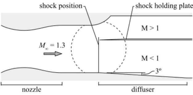
Experiments were performed in the No. 1 Supersonic Wind Tunnel at Cambridge University Engineering Department. This is a blow-down tunnel, capable of operating at Mach numbers between 0.7 and 3.5 depending on the chosen nozzle geometry. For the present work, the Mach number was fixed at M₁= 1.3, which was shown in [16] to give a representative shock strength for the airfoil model employed in the computations (described in section B.). The stagnation pressure of the flow was 172kPa, and the stagnation temperature was 300K; the Reynolds number was approximately 25 million m 1_{. Although,}

as described in [16], boundary layer suction could be employed to either manipulate the boundary layer ahead of the bump (at “in-flow”) or reduce the influence of corner flows, it was not used in this work. A schematic of the wind tunnel working section is shown in figure 5.

M < 1 M > 1 M = 1.3

nozzle diffuser

3º

shock holding plate shock position

Figure 5: Wind tunnel working section

Bumps were manufactured from VeroWhite resin, a non soluble opaque plastic, using a Polyjet rapid prototyping technique. These were glued to the wind tunnel floor using superglue, with the position accurate to within 0.5mm. A small amount of epoxy filler was used to give a smooth transition between the floor and the bump, although this was kept to a minimum to avoid interfering with the temperature-sensitive measurement techniques.

An array of methods were employed to measure the flow field. A two-mirror schlieren system with horizontal knife-edge was used to visualise the shock waves; this enabled the main normal shock position to be set to within _±1mm, as well as giving an indication of the ( )-shock structure generated by the bumps tested. Skin friction lines were examined by surface oil flow visualisation, using a mixture of paraffin, titanium dioxide and oleic acid.

Surface pressures were measured using single channel pressure sensitive paint (PSP), calibrated in-situ by a number of static pressure tappings. Di↵erent calibrations were performed for the (aluminium) wind tunnel floor and (plastic) bump surface, since the di↵erent thermal properties of the materials a↵ected the behaviour of the paint; the pressure field was then stitched together from the results of each calibration.

Velocity measurements were taken using two-component laser Doppler velocimetry (LDV), giving the streamwise and vertical velocities (uandv respectively). The flow was seeded with paraffin; the mean particle diameter was found to be approximately 0.5µm using measurements of particle lag through a normal shock, [21]. Boundary layer traverses were performed with variable measurement resolution between 0.2  y  0.5mm. The kinematic integral boundary layer parameters, equations 1, were calculated from this data using trapezoidal numerical integration with a correction factor applied to

account for the error introduced by the discretisation of the profile, following [22]. Full details of the experimental methods may be found in [16, 21].

⇤ i = Z 1 0 ✓ 1 u u1 ◆ dy , ✓i = Z 1 0 u u1 ✓ 1 u u1 ◆ dy , Hi= ⇤ i ✓i (1)

Errors in each of the parameters determined from experimental measurements are presented in table 1.

Table 1: Experimental errors

Quantity Source Error

Shock position image resolution, tunnel set-up ±0.2 0 Surface pressures PSP sensitivity, thermal e↵ects ±3% Streamwise velocity (u) LDA calibration, head angle ±1% Vertical velocity (v) LDA calibration, head angle ±10% B-L parameters ( ⇤

i, ✓i,Hi) LDA calibration, discretisation ±2.5%

B. Computations

Numerical simulations were performed at IAG, University of Stuttgart, for a streamwise cross section of the Pathfinder wing, a low-camber transonic design developed by a consortium of European research institutions as part of the TELFONA project for research on natural laminar flow wings and flow control, [23]. Computations were performed using FLOWer, a well-established density-based structured RANS flow solver developed by the German Aerospace Center (DLR), [24]. The two equation SST turbulence model due to Menter, [25], was chosen. No unsteady computations were required for the present work, except for the highest resolution used in the grid convergence study, where weak numerical damping required the addition of 100 inner unsteady iterations within the principal iteration loop.

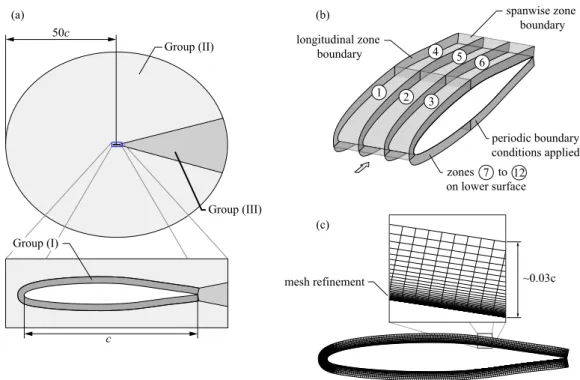
A multi-block structured C-grid, illustrated in figure 6, was used to enable parallelisation of the numerical solution. This was divided into twenty-seven zones, solved to second order accuracy within the zone and first order accuracy across zone boundaries. Twelve of these zones were distributed within 30mm of the wing surface (labelled group I on figure 6(a)); twelve were in the outer field (group II), which extended to a distance of 50c from the wing surface; and the wake region (group III) was divided into three equal sections across the span. The near-wing region carried mesh refinement in the boundary layer region, with the first grid point from the surface located aty+

⇡1. Periodic boundary conditions were specified on the spanwise limits of the domain, such that the set-up represents an infinite unswept wing.

50c c Group (II) Group (III) Group (I) 1 ₂ 4 3 5 ₆ longitudinal zone boundary spanwise zone boundary periodic boundary conditions applied 7 12 zones to on lower surface (a) (b) (c) ~0.03c mesh refinement

Figure 6: Details of the mesh used for computations

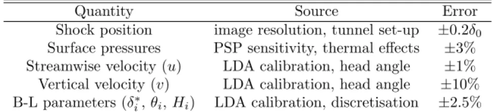
convergence study was performed, as first described in [16, 26]. This examined a dense reference (“level 0”) mesh consisting of 46 million cells, as well as three levels of coarsening: level 1 with 5.8 million cells; level 2 with 0.75 million; and level 3 with 0.1 million. The geometry tested was a HSCB as described in [16] positioned beneath the shock such that the flow is on the point of incipient shock-induced separation. This was chosen as separated flows are typically poorly modelled by RANS simulations and this therefore represents a ‘difficult’ test case for the CFD. Results of this study, in the form of profiles of cp andCf, are shown in figure 7, adapted from [16,26]. Level 3 fails to resolve the shock signature and completely misses the separation, whilst level 2 broadly captures the shock structure butCf does not get sufficiently low to suggest incipient separation. By contrast, level 1 is seen to capture both the shock structure’s pressure signature and the incipient separation observed in the dense level 0 mesh, although the shocks were slightly weaker as a result of a relatively coarse streamwise resolution. It was thus concluded that a mesh of 5.8 million cells would be the optimal trade between computational cost and solution accuracy, and this was duly applied for the remainder of the study.

Bumps are ‘mounted’ on the airfoil by displacing the relevant nodes in the mesh by an amount prescribed by a set of mathematical functions describing the SCB shape. They are placed symmetrically on the centreline of the domain, so that the e↵ective geometry is an infinite array of uniformly spaced bumps on the unswept wing.

Level 0 (unsteady) Level 1 Level 2 Level 3 0 -0.5 -1 0.5 1 0 0.2 0.4 0.6 0.8 1 x / c -cp (a) SCB main shock -5 0 5 10 15 0 0.2 0.4 0.6 0.8 1 x / c Cf (× 10 -3) (b) SCB

Figure 7: Results of the grid convergence study, adapted from [16, 26]

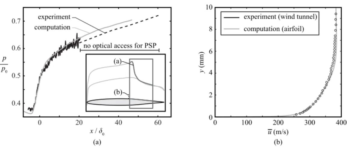
The flight conditions used are shown in table 2, which were chosen by [16] alongside the wind tunnel set-up to give good agreement between the computational and experimental uncontrolled flow fields. The agreement between the important features of the uncontrolled flow - the surface pressure distribution and boundary layer profile ahead of the SCB - are shown in figure 8, reproduced from [16]. The integral boundary layer parameters are compared in table 3. All length scales in the remainder of this paper are normalised by the in-flow boundary layer thickness, 0.

Table 2: Flight conditions used for numerical simulations

M₁ ↵[ ] xtrans/c Rec

0.76 1.8 0.1 20⇥106

Table 3: In-flow boundary layer properties ⇤ i ✓i Hi Re ⇤ i (mm) (mm) (mm) Exp. 6.0 0.67 0.53 1.28 27,650 CFD 6.0 0.67 0.51 1.31 25,670 C. Bump geometries

Three bump geometries were tested: the hill SCB (HSCB), wedge bump and extended SCB (exSCB), all shown in figure 9. The HSCB is a smooth contour bump originally defined by K¨oniget al., [8], the profiles of which are given by formulae for the bending of an elastic beam under a point load with di↵erent end conditions: the longitudinal profile has a ‘simply supported’ end at the bump nose and a clamped end at

0 20 40 60 0.4 0.5 0.6 0.7 p p₀ x / ₀ u (m/s) 0 100 200 300 400 0 6 8 10 2 4 y (mm) (b) (a)

experiment (wind tunnel) computation (airfoil) no optical access for PSP

(a) (b)

experiment computation

Figure 8: Comparison of uncontrolled flows in experiment and CFD: (a) surface pressure distribution; (b) in-flow boundary layer. Measurement locations shown inset.

the bump trailing edge; the lateral profile is simply supported on both sides. The wedge bump is similar to that used by various studies by Bruceet al., [9, 17]; all profiles are flat, except the side flanks which are cubic splines. The exSCB geometry is based on the wedge bump, except that the length and width of the tail have been increased. This was designed to make the flow locally more two-dimensional on the tail, thereby reducing pressure gradients and attenuating vortex production by the bump.

D. Vortex detection

A method of detecting vortices is required for analysis of the CFD data. It is well accepted that the existence of a maximum in streamwise vorticity!x=ex·r⇥uis a necessary but not sufficient condition for a vortex, with some pure shear flows also providing a maximum in !x - Jeong and Hussain, [27], in particular provide a number of examples. In the present work, the swirling strength criterion first proposed by Zhouet al. [28] is employed. This analyses the eigenvalues of the velocity gradient tensor, given by solutions to the characteristic equation:

3 ₍

r·u) 2+1

2((r·u)

2 _trace(

ru2)) det(ru) = 0 (2)

Let the solutions be_{ 1, 2, 3}, with corresponding eigenvectors{r1,r2,r3}. Then, if the solutions contain a complex conjugate pair ( 2 and 3, say) it can be shown that the flow field contains a spiral node in ther2 r3plane about which the flow swirls at rate₌( 2)_⌘ ci. Any point for which| ci|>0 may therefore be taken as belonging to a vortex core. Following [28], the vortices are visualised using plots of 2

33.33 ₀ 16.67 0 20 8.33 ₀ 11.67 ₀ 4.17 0 (c) (a) (b) 8.33 ₀ 15 ₀ C C A A 25 ₀ 12.5 ₀ 15.83₀ 8.33 0 15.83 ₀ 12.5 ₀ diffuser entrance shock positions 25 ₀ 4.17 0 8.33 0 8.33 ₀ 11.67₀ diffuser entrance shock positions 8.33 ₀ 11.67 ₀ diffuser entrance 0 Section A-A Section B-B Section C-C B B 0.83 ₀ 2.08 ₀ 40º 4.17 ₀ 40º crest geometry 0.83 ₀

Figure 9: Bump geometries tested: (a) HSCB; (b) wedge bump; (c) exSCB

as theQ-criterion and the enstrophyE.

III.

Comparison of CFD with experiments

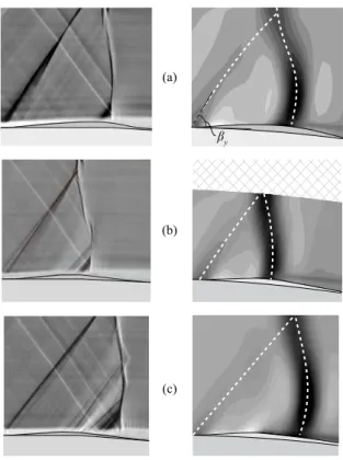
Figure 10 shows a comparison of the experimental and computational shock structures generated by the three bumps at o↵-design conditions (i.e. the shock in the downstream position). The experimental data was obtained by schlieren photography; the computational results show contours of the density gradients in the streamwise direction (i.e. ex·r⇢), mimicking schlieren with a vertical knife-edge†. The relatively low streamwise resolution used in the computations is apparent in the numerical schlieren images through the width of the shocks, although the results of the grid convergence study showed that †_{although the experiments were performed with a horizontal knife-edge, matching this in the computations did not} produce as clear a shock structure as that shown in figure 10 due to the streamwise mesh resolution

this does not present an issue for the surface pressure field or the impact on the boundary layer. There is a slight discrepancy which becomes apparent towards the top of the domain, caused by the underlying curvature of the airfoil surface in the CFD generating a small wall-normal pressure gradient that is not modelled in the wind tunnel. Nonetheless, the region of interest for this study (local to the boundary layer) is comparable: the angles of the front shock legs (indicated in figure 10) are given in table 4, from which a good level of agreement between the experiment and CFD is observed.

(a)

(b)

(c) y

Figure 10: Comparison of experimental and computational shock structures for three bumps at o↵-design condition: (a) HSCB; (b) wedge bump; (c) exSCB

Table 4: Front shock leg angles, y [ ], from experiment and CFD Experiment Computations

HSCB 57 59

wedge bump 59 59

exSCB 53 54

Surface flow topologies of the three bumps at o↵-design conditions are presented in figure 11. As has been remarked in previous studies, [9, 16, 17], the separation topology may be classified as an ‘owl-face of the first kind’ (see Perry and Hornung, [29]) comprising a pair of saddle points (markedS1 andS2 on figure 11) between which a region of reversed flow branches laterally to feed a pair of spiral nodes (F).

S1 F S2 S1 F S2 S1 F S2 S1 F S2 S1 F S2 S1 F S2 x_S1 L_S1-S2 z_F W_F

Figure 11: Surface flow visualisation from experiment and computations: (a) HSCB; (b) wedge bump; (c) exSCB

Whilst this is very clear for the HSCB and wedge bumps, on the exSCB the separation is divided into two separate parts with a channel of attached flow between them. Each of these separated regions has the owl-face topology. Because the separation entrains flow from the bump ramp, it must be open - i.e. the fociF feed a common-flow-up counter-rotating vortex pair into the flow.

For comparison purposes, the size of the separation may be categorized by the distance between the critical points: in particular the length is the streamwise distance between the saddle points, LS1 S2, whilst the width is the spanwise distance between the foci, WF (see figure 11). The position of the separation is categorized by the streamwise location ofS1,xS1, and the spanwise location of the spiral node zF. For the exSCB, the latter of these is measured for the closest spiral node to the centreline. These are compared for the computations and experimental results in table 5. In general, the CFD over-predicts the size of the separations, with first saddle point slightly further upstream than observed in the experiments.

Table 5: Comparison of separation sizes in computations and experiments

LS1 S2/ 0 WF± xS1 zF

Exp. CFD Exp. CFD Exp. CFD Exp. CFD

HSCB 9.5 13.7 4.0 4.3 17.0 16.0 2.3 2.2

wedge 7.3 17.7 5.0 4.9 12.3 10.4 2.7 2.4

exSCB 3.3 3.8 0.8 1.7 15.8 15.9 2.3 1.7

The surface pressure fields for the on-design cases of all the bumps are shown in figure 12. In general the agreement between the experiments and computations is good, particularly with respect to the shape of the flow (seen in the surface fields) and the pressure gradients away from the shocks (seen in the centreline distributions). However, there are some minor discrepancies: The shock is more smeared in the numerical results, doubtless a consequence of the streamwise mesh resolution. Notably, the pressure is over-predicted by the CFD on the bump tail - this is thought to be caused by a combination of slight di↵erences in shock position between the experiment and computation, as well as some minor influence of the wind tunnel side-walls in the experimental results.

A final comparison between the wind tunnel and numerical data is in the state of the boundary layer downstream of the bumps; measurements of this at x/ 0 = 28.33 are presented in figure 13. The horizontal dashed lines in figure 13 indicate the mean boundary layer parameters for the uncontrolled flow from both computational and experimental results. The computations are seen to over-predict the boundary layer parameters, and this is thought to be due to two e↵ects. Firstly, the curvature of the airfoil surface induces a wall-normal pressure gradient which will distort the boundary layer and thus increase both its displacement thickness ( ⇤i) and shape factor (Hi); the wind tunnel walls are flat, so this e↵ect is not present in the experiment. Secondly, there appears to be a tendency of the RANS computations used in the present work to over-predict the increase in the integral parameters through the shock/boundary layer interaction, [21]; this can be seen here by the di↵erence in the uncontrolled values of ⇤

i andHi. However, if the change in the integral parameters relative to the uncontrolled flow is considered (i.e. the direct impact of the SCB), then the agreement between CFD and experiment is seen to be better.

For the purpose of the present study, the shock smearing due to the streamwise resolution of the CFD is likely to be the most severe limitation. Consequently all analysis of pressure gradients - particularly in section V. - will be restricted to regions away from the shock footprints as well as on the surface. The above comparisons with PSP data shows that if such precautions are taken, the CFD and the experiments generally agree quite well in the shape of the flow, whilst the grid convergence study analysis also suggests

0.3 0.4 0.5 0.6 0.7 p p₀ 0 10 20 30 x / ₀ 0 10 20 30 x / ₀ 0 10 20 30 x / ₀ (a) (b) (c) 0.3 0.4 0.5 0.6 0.7 p / p₀ CFD exp CFD exp CFD exp

SCB extent SCB extent SCB extent

Figure 12: Surface pressure fields from experiment (top row), CFD (middle row) and centreline distri-butions (bottom row): (a) HSCB; (b) wedge bump; (c) exSCB

4 6 8 10 1.6 2.4 2 2.8 0 2 4 -2 -4 z / ₀ z / ₀ i * * i,0 i 0 2 4 -2 -4 z / ₀ 0 2 4 -2 -4

Figure 13: Integral boundary layer parameters across the span atx/ 0= 28.33, symbols show experimen-tal data; lines show computations: (a) HSCB; (b) wedge bump; (c) exSCB. Horizonexperimen-tal dashed lines show the state of the boundary layer in the uncontrolled flow from experiments (light grey) and computations (dark grey).

a similar conclusion. Finally, the resolution is the same relative to the bump length scales for all cases tested, which ensures a safer comparison between geometries. It is therefore not expected that the shock

resolution will present a significant problem to the analysis of the present work.

IV.

Vortical flow structures

A. Design behaviour

Attention is now turned to the vortical flow structures generated by the bumps. Since it would be prohibitively expensive to gather sufficient data to build a complete picture of the flow structures, the computational data is used to provide an overview of the flow field. Contours of both the streamwise component of vorticity, !x =ex·r ⇥u, are presented in figure 14, as well as contours of the swirling strength vortex sensor, 2

ci. No contour levels are shown for the latter as it is intended as a qualitative guide to the flow features.

(a) (b) (c) 1 0.5 0 -0.5 -1 x (×103₎ (I) (II) (II) (IV) (IV) (III) (III) (I) (IV) (IV) (II*) (IV) (IV)

Figure 14: Vortical structures on SCBs under design conditions visualized by contours of!x (top row)

and 2

ci(bottom row): (a) HSCB; (b) wedge bump; (c) exSCB

A number of flow structures common to all the bumps are visible:

(I) shear flow caused by the curved front ( )-shock leg

are weak secondary vortices detected for the HSCB and a more noticeable vortex for the exSCB (labelled (II*) in figure 14(c))

(III) centreline shear flow, associated with having a flat section between the bump flanks - this only appears on the wedge and exSCB, but not the HSCB which has continuous surface curvature over the bump width

(IV) primary vortex - the dominant vortical structure in the wake for all SCBs tested

The contours of 2

ci show that only the primary vortices are of importance for potential boundary layer control, since this is the only structure relating to streamwise vortices that persists into the wake. Some key characteristics of these vortices, extracted from the data in figure 14, are shown in table 6. The maximum streamwise vorticity is the peak observed in the primary vortex structure 5hdownstream of the bump trailing edge. The circulation shown is evaluated for a circuit enclosing half the domain -from the centreline to the domain edge - and extending to a height of 5 0 to capture all of the vortical structures. The results are non-dimensionalised using the bump height hand the skin friction velocity of the uncontrolled flow at the same point on the airfoilu⌧.

Table 6: Characteristics of primary vortices under design conditions, measured 5hSCB downstream of the bump trailing edge

!x,max /(u⌧h)

HSCB 1200 3.61

wedge 1998 3.76

exSCB 1500 1.79

These results suggest that the vortices are remarkably strong, considering that the bumps have not been designed to optimise vortex production. To put the magnitudes into context, a typical sub-boundary layer VG might have a non-dimensional circulation of around 20. The integration also includes contributions from flow structures of the opposite sense (that this will happen is clear from figure 14) which will detract from the overall calculated circulation at this point; hence the values given above are likely to be underestimates of the true primary vortex strengths.

The presence of the primary vortices is well-documented for the HSCB and wedge type bumps (see, for example, Bruce and Babinsky [9], Collisset al.[16]); however, for the exSCB its presence is somewhat troubling within the framework of current bump physics understanding. As seen in the introduction to this paper, the consensus in the literature is that spanwise pressure gradients over the tail section of the bumps are responsible for generating and controlling the streamwise vortices. In increasing the

length and width of the bump tail - as for the exSCB - these pressure gradients should be reduced, thus attenuating the production of streamwise vortices. Structure (IV) should not therefore be observed, yet there is clear evidence of it in figure 14 and moreover it is seen to be quite strong in table 6. This suggests that the current understanding of vortex production may be incomplete or incorrect, and this is something that will be investigated further (see section V.).

B. O↵-design behaviour

The streamwise vorticity and swirling strength contour maps for o↵-design conditions are shown in figure 15. (a) (b) (c) 1 0.5 0 -0.5 -1 x (×103₎ (I) (III) (I) (V) (V) (II*) (IV) (IV) (V) (V) (IV) (V) (III+V) (IV) (II) (II)

Figure 15: Vortical structures on SCBs under o↵-design conditions visualized by contours of !x (top row) and 2

ci (bottom row): (a) HSCB; (b) wedge bump; (c) exSCB

As labelled in the figure, most of the flow structures observed for the on-design case are once again visible here. In particular, for all bumps the vorticity within the ( )-shock (structure (I)) is unchanged from design conditions (as should be the case), whilst the secondary vorticity (II) can also be identified. The key di↵erence from design conditions is around the flow separation on the bump tails. The details of this were shown in figure 11, and it was stated that the separation topology should produce a

common-flow-down vortex pair: this can be observed in the figure 15, labelled (V).

For the HSCB and wedge bump, structure (V) is seen to dissipate relatively rapidly downstream in the 2

ci data. In both cases the vortex is seen to have decayed by around 0.25LSCB downstream of the tail, although on the wedge bump there is still a high peak in !x at, and downstream of, this location. This is caused by the presence of shear, observed in the on-design case as structure (III).

On the exSCB, structure (V) persists far downstream - indeed it is the primary constituent of the wake. Examining the rotation of the vortices (using !x), it can be inferred that the inner vortices emanating from the two separations (i.e. those closest to the centreline) are dominant, with the others (the ones closest to the bump flanks) being indistinguishable in both the!x and 2cidata, and therefore very weak. The result is that the net wake structure is a common-flow-down vortex pair, similar to the on-design case, but generated in a very di↵erent way.

Because of the decay of the separation vortices on the HSCB and wedge bump, the wake structure is dominated by flow features which are not caused by the separation. This comprises a common-flow-down pair of vortices which appear similar in character to those generated in the on-design case. In fact, these can be identified with those of the on-design case, due to their similarity in character and position, hence are labelled (IV) in figure 15.

This is a particularly interesting observation because it shows that even if the flow on the bump tail separates, thus radically changing the e↵ective aerodynamic shape of the tail, the primary vortex structure is still generated. As with the generation of vortices on the exSCB under design conditions, this seemingly contradicts the understanding that the SCB tail is responsible for generating the vortices.

V.

Factors influencing vorticity

In order to investigate the apparent anomalies of vortex production noted in the previous section, a number of parametric variations of the bumps tested in this paper have been examined, looking at the relationship between pressure gradients at various locations and the strength of the vortices generated. Figure 16 shows the SCB geometries and the key geometry dimensions varied; table 7 shows the values of the dimensions tested; the domain width (which is e↵ectively the lateral bump spacing due to the periodic boundary conditions) is denoted b and not shown on the figure. The data is collected from numerical simulations, since the relatively inexpensive nature of the CFD enabled a larger number of bumps to be examined.

(a) (b) (c) h w L L_ramp L_ramp w_tail w h w_tail

Figure 16: SCB geometries and key dimensions

Table 7: Dimensions of bumps tested and symbols used in figure??

Symbol SCB type L/ 0 w/ 0 h/ 0 b/ 0 Lramp/ 0 wtail/ 0

HSCB 25 8.33 0.5 16.67 12.5 8.33 25 8.33 0.67 16.67 12.5 8.33 25 8.33 1 16.67 12.5 8.33 25 8.33 1.33 16.67 12.5 8.33 25 8.33 1.5 16.67 12.5 8.33 25 8.33 0.67 25 12.5 8.33 25 8.33 1 25 12.5 8.33 25 8.33 1.33 25 12.5 8.33 50 16.67 3 25 25 16.67 wedge 25 8.33 0.83 16.67 8.33 4.17 25 8.33 0.83 25 8.33 4.17 exSCB 33.33 4.17 0.83 16.67 8.33 16.67

to be particularly representative: these are shown in figure 17. The streamwise pressure gradient on the tail was measured half way between the shock location and the bump trailing edge, on the centreline of the bump (figure 17(a)). The tail spanwise pressure gradient was measured at the same streamwise location, but taken at the spanwise location directly beneath the peak vorticity within the primary vortex core (figure 17(b)). . Spanwise pressure gradients on the bump ramp are characterised by the highest pressure gradient observed half way between the bump nose and the shock, i.e. x = xs/2 (figure 17(c)). Any pressure gradients taken through the front ( )-shock leg are discarded, such that the pressure gradient recorded is always on the bump surface (and usually on the bump flanks). Although the streamwise location ofxs/2 is quite arbitrary, it was found that examining points ahead or behind this (which avoided interference with the region with either forward or rearward shock leg) produced a similar result.

x_s / 2 x_s L_rear L_rear / 2 (a) p/ x (c) p/ z (b) p/ z primary vortex x shock leg max gradient data excluded p z z y ( )-shock footprint

Figure 17: Pressure gradients and locations tested, as labelled: (a) streamwise pressure gradient on tail; (b) spanwise pressure gradient on tail; (c) spanwise pressure gradient on ramp.

using 2

ci, both for identifying the appropriate peak in!x for the primary vortex core (as in figures 14 and 15) and for ensuring that the vorticity recorded was representative of the swirl itself. The latter was done using the fact that !x,swirl is twice the rotation rate of a fluid packet, i.e. 2 ci. The vortex strengths were then plotted against the various pressure gradients of figure 17, shown in figures 18 and 19. In addition, the maximum vorticity has been plotted against the shock location (relative to the bump length) for the HSCBs withL/ 0= 25.

1 p₀ p x x_s L x (10 3 s -1) (a) 0 1 2 3 4 5 x (10 3 s -1) 0 1 2 3 4 5 1.6 0 0.1 0.2 0.3 0.4 0.5 0.6 0.7 0.4 0.8 1.2 (b)

Figure 18: Correlations of vortex strength with: (a)@p/@xon tail; (b)xs/L. Open symbols represent unseparated flows; closed symbols represent flows where separation occurs on the bump tail.

No trend with the streamwise pressure gradient is seen to exist - the ‘best fit’ line drawn on figure 18(a) has a very low correlation coefficient (R2 _{= 0.096) and in fact similar correlation coefficients could} obtained with a more horizontal line; this indicates that the data is more of a random point cloud. Moreover, when the maximum streamwise vorticity is plotted against the shock location, there remains no discernible trend. Given the significant variation in the local pressure gradients on the bump tail that the shock location can generate, this suggests that the streamwise gradient may be of little or no importance to the vortex generation. It therefore appears that the spanwise pressure gradients are the most important for the generation of vortices by SCBs.

1 p₀ p z 1 p₀ p z x (10 3 s -1) (a) (b) 0 1 2 3 4 5 0 0.1 0.2 0.3 0.4 0 0.4 0.8 1.2 1.6 2

Figure 19: Correlations of vortex strength against pressure gradients: (a) @p/@xon tail; (b)@p/@z on tail; (c) @p/@z on ramp. Open symbols represent unseparated flows; closed symbols represent flows where separation occurs on the bump tail.

The spanwise pressure gradient on the tail shows more of a linear trend, although the correlation coefficient is still not particularly high in this case (R2_{= 0.421). A much stronger correlation is observed} for the spanwise pressure gradients on the ramp (for whichR2_{= 0.885). This suggests that it is actually} the flow on the bumpramp which governs the formation of streamwise vortices in the wake, rather than that on the tail as was previously thought.

The above analysis immediately explains the apparently anomalous observations made earlier in this paper. The exSCB has a wider and longer tail, leading to lower local pressure gradients, but it still produces vortices because the ramp section is of similar geometry to the wedge bump. Likewise, the appearance of boundary layer separation on the bump tails under o↵-design conditions does not significantly alter the vortex production, because this is governed by what is happening ahead of the shock, which is of course unchanged.

This result is significant because it means that the flow control potential of a SCB is decoupled from the bump’s e↵ect on the boundary layer, which is controlled by the tail ( [7, 9, 17]). In particular, the ramp geometry determines the inviscid control potential of the bump, governed by the ( )-shock characteristics, as well as the boundary layer control potential of the bump, governed by the vortices in the wake.

VI.

Conclusions

Computational results for a number of SCB geometries have been examined to understand the flow structures generated by the bumps as well as investigate the factors governing the properties of their wakes. A joint experimental and numerical approach developed and tested previously was used to validate the computational data prior to investigating the details of the flow. Three bump geometries were tested: hill (smooth contour), wedge and extended bumps. Two shock positions were considered, the ‘design’ condition where the shock sits at the crest; and the ‘o↵-design’ condition where the shock is sufficiently far downstream of the crest to cause a localised flow separation.

It was found that under design conditions all bumps produce three principal flow structures: shear flow within the ( )-shock caused by the curvature of the front shock leg; shear emanating from the bump tail around the crest region; and primary vortices, which are the main constituent of the wake. The wedge and extended bumps also generated a region of weak shear on the flat section in between the side flanks which was not present on the HSCB (due to the continuous surface curvature across the span). That the exSCB produced a primary vortex pair at all was in conflict with the understanding that the bump tail is responsible for generating the vortices.

Under o↵-design conditions, the presence of flow separation modified the wake flow structure, prin-cipally through the addition of a common-flow-up counter-rotating vortex pair emanating from the separation topology. This had the same form for the hill and wedge bumps, although the increased width of the extended bump tail lead to the topology being localised to the bump flanks and duplicated on either side such that the vortices closest to the centreline dominate, with a region of attached flow in between. This directly resulted in the wake being dominated by a common-flow-down vortex pair on the exSCB. The HSCB and wedge bump’s separation vortices were seen to decay quickly, however, with the primary vortex pair like that generated under design conditions being the main component of the wake. Thus all the bumps tested behave like vortex generators, creating a rotationally similar structure in all cases even when the boundary layer separation on the tail modifies its e↵ective aerodynamic shape. This

is also in conflict with previous explanations of vortex production by SCBs.

The strength of the primary vortices for all bumps at design conditions was found to be around 20% of that of a typical vortex generator, surprisingly strong given that none of the bumps in this study were designed or optimised for vortex production. A number of parametric modifications of the bumps were made and the strengths of the vortices produced by each of the bumps in the resulting database were correlated against pressure gradients at various locations on the bump. It was found that the vorticity is most strongly related to spanwise pressure gradients on the bump ramp, suggesting that it is the front of the bump which is responsible for generating the streamwise vortices and not the tail, as was previously thought to be the case.

Acknowledgments

The research leading to these results has received funding from the European Union’s Seventh Frame-work Programme (FP7/2007-2013) for the Clean Sky Joint Technology Initiative as part of the NextWing program under grant agreement no. 271843.

References

[1] Stanewsky, E., D´elery, J., Fulkner, J., and Geissler, W.,Synopsis of the project Euroshock, Results of the project EUROSHOCK, Vol 80 ofNotes on numerical fluid mechanics: drag reduction by passive

shock control, pp. 1–124, 2002.

[2] Caruana, D., Mignosi, A., Corr`ege, M., Le Pourhiet, A. and Rodde, A.M.,Bu↵et and bu↵eting control

in transonic flow,Progress in Aerospace Science, Vol 9, pp. 605–616, 2005.

[3] Lee, B.H.K., Self-sustained shock oscillations on airfoils at transonic speeds, Progress in Aerospace

Sciences, Vol 37, pp. 147–196, 2001.

[4] Bogdanski, S., N¨ubler, K., Lutz, T. and Kr¨amer, E.,Numerical investigation of the influence of shock

control bumps on the bu↵et characteristics of transonic airfoils,Notes on Numerical Fluid Mechanics

and Multidisciplinary Design, Vol 124, 2014.

[5] Stanewsky, E., D´elery , J., Fulkner, J. and de Matteis, P.Synopsis of the project EUROSHOCK II, Results of the project EUROSHOCK II, Vol 56 ofNotes on numerical fluid mechanics and

[6] Birkemeyer, J., Rosemann, H. and Stanewsky, E.,Shock control on a swept wing,J. Aerospace Science

and Technology, Vol 4, pp.147–156, 2000.

[7] Ogawa, H., Babinsky, H., P¨atzold, M. and Lutz, T., Shock-wave/boundary-layer interaction control

using three-dimensional bumps for transonic wings,AIAA J., Vol 46, No 6, pp. 1442–1452, 2008.

[8] K¨onig, B., P¨atzold, M., Lutz, T. and Kr¨amer, E., Numerical and experimental validation of

three-dimensional shock control bumps,J. Aircraft, Vol 46, No 2, pp.675–682, 2009.

[9] Bruce, P.J.K. and Babinsky, H., An experimental study into the flow physics of three-dimensional

shock control bumps,J. Aircraft, Vol 49, No 5, pp. 1222-1233, 2012.

[10] Eastwood, J.P. and Jarrett, J.P.,Towards designing with 3D bumps for lift/drag improvement and

bu↵et alleviation,AIAA J., Vol 50, No 12, pp. 2882–2898, 2012.

[11] Henderson, L.F., and Meniko↵, R., Triple shock entropy theorem and its consequences, J. Fluid

Mech., Vol 366, pp.179–220, 1998.

[12] Qin, N., Wong, W.S., and Le Moigne, A.,Three-dimensional contour bumps for transonic wing drag

reduction,Proceedings of the Institute of Mechanical Engineers, Part G - Aerospace Enginering, Vol

222, pp. 619–629, 2008.

[13] Qin, N., Zhu, Y, and Ashill, P.R.,CFD study of shock control at Cranfield, ICAS Paper 2000-2105, 2000.

[14] Sommerer, A., Lutz, T., and Wagner, S.,Numerical optimisation of adaptive transonic airfoils with

variable camber, ICAS Paper 2000-2111, 2000.

[15] Bruce, P.J.K., and Colliss, S.P., Review of research on shock control bumps, Shock Waves Journal, DOI 10.1007/s00193-014-0533-4, 2014.

[16] Colliss, S.P., Babinsky, H., N¨ubler, K. and Lutz, T., Joint approach to three-dimensional shock

control bump research,AIAA J., Vol 52, No. 2, pp. 432–442, 2014.

[17] Bruce, P.J.K., Colliss, S.P. and Babinsky, H.,Shock control bumps: e↵ects of geometry, 52nd AIAA Aerospace Sciences Meeting, National Harbour, Maryland, AIAA Paper 2014-943, 2014.

[18] Wong, W.S., Qin, N., Sellars, N., Holden, H. and Babinsky, H., A combined experimental and

numerical study of flow structures over three-dimensional shock control bumps, Aerospace Sci. and

[19] Ogawa, H. and Babinsky, H.,SBLI control for wings and inlets, In: Shock waves: 26th international symposium on shock waves, Vol 1, pp.51–57, Springer, 2009.

[20] Eastwood, J.P.,3D shock control bumps: bridging the gap between lift/drag improvement and bu↵et

alleviation?, PhD Thesis, University of Cambridge, 2012.

[21] Colliss, S.P.,Vortical structures on three-dimensional shock control bumps, PhD Thesis, University of Cambridge, 2014.

[22] Titchener, N.A., Colliss, S.P., and Babinsky, H., On the calculation of integral boundary layer

parameters from discrete data,Experiments in Fluids, Vol 56, No 8, 2015.

[23] Perraud, J., Archambaud, J.-P., Schrauf, G., Donelli, R., Hanifi, A., Quest, J., Streit, T., Hein, S., Fey, U., and Egami, Y.,Transonic high Reynolds number transition experiments in the ETW cryogenic

wind tunnel, 48th AIAA Aerospace Sciences Meeting, Orlando, Florida, AIAA Paper 2010-1300, 2010.

[24] Kroll, N. and Fassbender, J.K., Part II of MEGAFLOW, Vol. 89 of Numerical flow simulation for

aircraft design, pp. 25–77, Springer-Verlag, Berlin, 2005.

[25] Menter, F., Two-equation eddy-viscosity turbulence models for engineering applications, AIAA J., Vol 32, No 8, pp. 1595–1605, 1994.

[26] N¨ubler, K., Colliss, S.P., Lutz, T., Babinsky, H., and Kr¨amer, E.,Numerical and experimental

exam-ination of shock control bump flow physics,High Performance Computing in Science and Engineering

‘12, Springer, Berlin Heidelberg, DOI 10.1007/978-3-642-33374-3 25, 2013.

[27] Jeong, J. and Hussain, F., On the identification of a vortex, J. Fluid Mech., Vol 285, pp. 69–94, 1995.

[28] Zhou, J., Adrian, R.J., Balachandar, S., and Kendall, T.M., Mechanisms for generation coherent

packets of hairpin vortices, J. Fluid Mech., Volume 387, pp. 353–396, 1999.

[29] Hornung, H. and Perry, A.E., Some aspects of three-dimensional flow separations, part II: vortex