An Econometric Evaluation of Women s Labour Supply in WA

(1)

An Econometric Evaluation of

Women’s Labour Supply in WA

A Report Prepared for the Western

Australia Department of Consumer

and Employment Protection

Laurence Lester and Darcy Fitzpatrick

23 July 2008

(2)

An Econometric Evaluation of Women’s Labour Supply in WA

A Report Prepared for the Western Australia Department of

Consumer and Employment Protection

Laurence Lester and Darcy Fitzpatrick

National Institute of Labour Studies

1

23 July 2008

List of Tables

Table 1—HILDA Observations (Combined Waves 1 to 6) 7

Table 2—Legend: Explanatory Variables Used in Econometric Models 16

Table 3—Summary Statistics for WA and Australia 18

Table 4—Participation: Single and Couple Females—WA and Australia 24

Table 5—Hours Worked: Single and Couple Females—WA and Australia 35

(3)

Executive Summary

Following a comprehensive review of the recent theoretical and applied econometric literature, we use sophisticated panel (longitudinal) data econometric models to examine factors affecting female labour force participation and hours of labour supply for Western Australia (WA) and Australia.

Labour supply behaviour of females differs to that of males, and the behaviour of single females differs to that of females with partners. Notwithstanding the changes in forms of employment over the last decade, female labour force participation and hours work are significantly lower than for males. Moreover, a greater proportion of single females work full-time hours compared to females with partners, and single females generally work more hours per week compared to females with partners. Child-rearing is generally undertaken by females, and childcare responsibilities continue throughout much of the female’s working age life thus partially explaining lower average rates of labour market activity of females.

This Report examines which factors explain labour force participation and of hours of work of single and partnered females, with or without dependants, of age 18-64 years (excluding full-time students and self-employed females) using the six annual (2001-2006) waves of the Household, Income and Labour Dynamics in Australia (HILDA) survey data.

In the HILDA data, the WA sample is small in comparison with the preferred sample size used in empirical research directed at labour market issues. Therefore, notwithstanding the aim of this Report is to provide distinct analysis for WA, models for Australia are likely to be a superior guide to underlying drivers of labour market behaviour and to provide indicators of directions for further research, and implications for policy directions.

In this Report, econometric models issues such as “sample selection bias” (female supply hours of work are not a random selection from the population), unobserved individual characteristics (unobserved heterogeneity), and dynamics of behaviour are controlled so that econometric model estimates are unbiased and reliable, leading to dependable conclusions. When models are estimated, a number of issues are dealt with at a more refined level than necessarily included in previous studies—and issues not always included in previous analysis are examined. For example, the influence on hours of work supplied of maternity leave, union membership, and immigrant’s length of residence in Australia are examined.

While the econometric results in this Report are robust, several areas where further research is warranted are identified. For example, the analysis of female hours of work is estimated based on the “unitary” labour supply model: although, the more recent literature suggests a “collective” model of household labour supply is more appropriate for couple-households (with or without children), currently available econometric software precludes the use of this more advanced approach.

Female Labour Force Participation

Models for female labour force participation require adjustment for labour market dynamics, but no underlying trend in participation was found for the six-year period of the HILDA data.

(4)

A number of factors are confirmed as influences on female participation including, years of work experience, education, non-labour income, health, non-residential children, and marital status.

Generally, children below five years of age reduce couple females’ participation, but children over five years of age increase participation. Single Australian females do not appear to be influenced by children below the age of five years, but increase participation for children between 15 and 24 years. WA single females’ results differ (e.g. children below age five reduce participation, but older children have no impact). This is an area where further investigation would be useful (e.g. interaction effects such as access to childcare).

The immigrant’s period of residence was strongly influential in the Australian, but not the WA, models of participation (the WA result is probably due to a small sample exacerbated by immigrants making up a small proportion of the sample). Thus, government-provided access to English language tuition, job search skills, and information about the operation of the Australian labour market may increase the participation of immigrant females to that of otherwise similar non-immigrants. This method of measuring the impact of being an immigrant is an innovation and is an area where further research may be valuable.

Interestingly, there appears to be little if any impact of partner’s attributes on participation: partner’s education plays no role; partner’s non-resident children play no role; and although partner’s wage is statistically significant for WA couple females, the impact is quite small. Nonetheless, marital status always matters for couple females hence suggesting an inter-dependence of female and partner’s decisions and hence supporting use of the “collective” labour supply models when the limitations imposed by currently available theory and software can be overcome (see further comments below).

Conventional wisdom is that single and couple females have different patterns of labour force participation. It is clear from the models for Australia and WA that there are surprising similarities, but there remain distinct differences for single and couple females (e.g. non-labour income has a larger impact for single females than couple females).

In summary, although there are, for both Australia and WA, a number of similarities in the model estimates for single females and couple females, there are important differences. Failure to model singles and couples separately is an aggregation problem leading to potentially incorrect inference and misguided policy analysis and recommendations.

Policy implications arising from the analysis of female labour force participation tend to follow the literature—there are limits to potential intervention, and most policy can at best be directed to longer-term issues. For example, education generally increases the probability of labour force participation, but education (and associated vocational skills development) is not subject to short-run manipulation. Similarly, very young children in a household reduces the participation rate of females, but whether there is a long-term advantage to pursue methods to increase the participation of this group is a complex question, as is the issue of what influences the decision to have a child and its relationship to labour market participation. Examination of the model results does not suggest any particularly striking differences in drivers of labour force participation between Australia and WA females for single or partnered females.

(5)

Supply of Hours of Paid Work

Econometric models examine the impact of selected determinants on females’ supply of hours of paid work per week for the sub-sample of females who are employed.

As with labour force participation, dynamics must be accounted for in models, but there is no evidence of a consistent underlying trend in hours supplied (except for an irregular reduction in hours worked for single females in WA across the waves of data). Similarly, examination of hours supplied confirms the appropriateness of modelling single and partnered females separately.

Not all partner’s attributes include in the models are significant influences on female hours of work, but they are not irrelevant—and in conjunction with the participation equation (and the employment equation used to ensure hours supplied equations do not suffer from selection bias) suggest a tendency for inter-dependence of female and partner’s labour market decisions. This supports further research using “collective” labour supply models to obtain more efficient and robust estimates, and to observe intra-household welfare allocations (when, in particular, software to estimate appropriate models is available).

Some factors influence females’ probability of labour force participation, but do not have a further impact on hours supplied, e.g. non-labour income has no impact, and education has a much reduced impact.

Mental health appears to have no impact on the number of hours supplied. This result is at odds with common understanding of the influence of stress in the workplace. The influence of physical health also requires further research: while results are consistent for three of the four models (and influence participation as expected), they are counter intuitive: good health implies reduces hours of labour supplied. The impact of mental and physical health requires further investigation.

The influence of children at home on hours supplied depends, as expected, on the age of the children. For example, for Australian couple females, an own-child at home reduce the number of hours worked, but the impact of children for single females is about half that of couple females for children to age 14—with no impact of children age 15 to 24. Results appear to differ for the WA models—this is a case where the Australian results probably are more reliable to sample size issues (combined with the distribution of children across the samples). The presence of non-residential own or partner’s children have little impact on hours supplied, being significant in only the Australia couple females model.

The direction of the impact of age on hours supplied is generally consistent across specifications, but the size of the impact varies with model specification (e.g. a one year increase in age increase hours supplied by two per cent for Australia single and couple females, and by six per cent for WA single females, but for WA couples there is a perverse 6 per cent reduction). The Australian results should be considered more reliable. Diminishing returns to age are generally observed, but the impact is very small. An implication from age results is that industry’s apparent preference for younger workers is counter-productive. It is often due to discrimination, as employers simply assume older workers are less productive. Hours worked by females may be increased by demand side policy that influence industry’s reported negative attitude to older workers.

(6)

The impact of being an immigrant differs in models for Australia and WA (the Australian result is probably more reliable). Where significant, in contrast with the impact on participation, as the length of residence increases the number of hours supplied decreases. The reason for this outcome is unknown and warrants further investigation.

Wage rates matters only in the Australian couple model—and the direction of the influence is consistent with the “backward bending” labour supply curve associated with higher level wage earners. The lack of influence for single females suggests a lack of access to other sources of income curtails their ability to reduce hours, but neither do they increase hours when wage increases suggesting they are “time poor”. The issue of the impact of wage on hours supplied may be complex and requires further investigation.

All models demonstrate that the availability of paid or unpaid maternity leave is an important influence on hours supplied by both single and couple females. In addition, partner’s paternity leave is influential for Australian couple females, but the result is counter-intuitive: the availability of leave reduces hours supplied. As maternity leave is an area that could be influenced by government intervention the importance of the availability of such leave requires further investigation. Thus, for example, as well as more detailed specification of leave entitlements in econometric specifications, the interaction between industry sector and leave could be considered—are there industries where greater attention should be directed? There are other influences on hours supplied, although there is little if any scope to influence them, directly or indirectly, and hence no avenue for policy intervention. Nonetheless, their absence in previous models is a model misspecification—leading to unreliable econometric results. Factors considered are trade union membership (generally, a positive influence on hours worked); industry sector, and in the Australian models state of residence.

In summary, as with the participation models, there are, generally (but not necessarily across the four models or sub-samples) a number of similarities for single and couple females behaviour with respect to hours of work supplied (e.g. control for dynamics and “state dependency”, trend, non-residential “own” children, health, age, maternity leave, and impact of being an immigrant). On the other hand, there are important differences for single and couple females (e.g. the impact of children, education, non-labour income, wage, employed in the public or private, state of residence, and industry).

Conclusion

This Report is based on estimating labour force participation and supply of hours of paid work equations for single and couple females in Western Australia and Australia. The Report provides justification for the econometric models chosen and discusses the limitations of the models and the ensuing results. Throughout, references are made to a number of issues that should be considered for future research to extend the scope of this work.

To the extent possible, given current theoretical and applied limitations, models reported are based on recent advances in both theoretical and practical applications of panel (longitudinal) data econometric models. Notwithstanding constraints, the models are an advance on previous methods, and so provide econometric model results that are more reliable: biases due to model misspecification (including missing variables), unobserved heterogeneity, selection bias, and dynamics and “state dependency”, have been addressed.

(7)

A number of innovations in this Report (beyond the use of advanced modelling techniques) provide added perspective on the hours supplied decision of females. For example, the availability of maternity leave has an impact in all hours of supply equations, and the period of residence of immigrants is also influential (via a more detailed method of including immigrants’ in models not previous considered).

Overall, the model results clearly indicate that female data must be disaggregated to single and couple females sub-samples. Although the explanatory power of several important explanatory variables is not different across single and couple female models, a sufficient number differ importantly—aggregation of single and couple females results in “aggregation bias” and unreliable econometric estimates.

The Report provides interesting insights to females’ behaviour, and suggests some areas where government policy intervention may contribute to increased hours supplied—for example, maternity leave and access to labour market skills for immigrants. Advances in theory and econometric practice are likely to provide appropriate, “collective” model which may lead to further insights into female labour market interactions and hence may suggest avenues for government intervention to increase hours of work.

On the other hand, the probability of labour force participation seems to suggest few areas where state government intervention could successfully influence participation. This area could be considered for further investigation.

Suggestions for further Research

The most important field for future research is to utilise recent theoretical extension of labour supply modelling, and move beyond the “unitary” approach to the “collective” approach. In the collective approach, labour market decisions of couples are made according to the power relationship, and not on the assumption that there is an entity, the household, that makes the “unitary” decision. Nonetheless, although theoretically advanced, impediments to constructing complex “collective” models exist, including the appropriate treatment of children, and designation of the internal balance of power which influences the decision making process. While such models are currently beyond “off the shelf” econometric packages, academic work continues, and testable specifications, and econometric package add-ons—are expected to become available.

Samples for smaller population state such as WA limit the application of advance models. Differential results for Australian females and WA females are probably due to small samples for WA and not necessarily differential behaviour, thus models for Australia may be satisfactorily informative. This constraint cannot be overcome without a large investment in state specific data collections—which, even if conducted, will require several years of data collection before there are sufficient data and time-period or waves of survey data to construct the necessarily complex models for female labour market interactions.

Finally, models for females have been examined. An important question for further research is consideration of the reaction of male partners to female’s changes in participation and hours supplied—if female increased participation or hours worked is at the expense of a reduction in male participation or hours the overall problem of shortages of supply are not addressed: which sector should be targeted?

(8)

The Work Undertaken

This National Institute of Labour Studies (NILS) “Report” for the Western Australian Department of Consumer and Employment Protection (DOCEP) presents the results of econometric modelling of female labour force participation and the supply of hours (contingent on being employed) for females in Western Australia (WA) and for Australia. We use sophisticated panel (longitudinal) data econometric models which are based on an extensive review of the recent theoretical and applied econometric literature addressing labour supply for single and partnered individuals.2 Applied econometric models of labour force participation and hours of labour supply in this Report:

a) investigate the set of factors which influence women’s decisions, the relative importance of explanatory factors, and implied semi-elasticities (i.e. the percent change in the dependent variable for a one unit change in an explanatory variable); b) control for unobserved individual level attributes or characteristics (i.e. unobserved

heterogeneity);

c) incorporate dynamics to control for the influence of previous period values and “state dependency”3 on the current value of the dependent variable;

d) adopt a two-stage selection model to account for potential bias in econometric estimates due to “selection bias” in models of hours of labour supply (i.e. labour supply is contingent on a labour force participant female being employed); and

e) analyses separate models for single females and for females with male partners. Following the report of the results of econometric modelling, we canvas the implications of the econometric model results for influencing the labour supply of women.

Background

Labour Supply Shortages—WA and Australia

The present shortage of labour in WA is an amplified version of that being experienced throughout Australia. Labour shortages, which present a serious problem from the point of view of employers, are a consequence of the surge in the demand for skilled workers from the above average annual rate of economic growth: for example, between 1992 and 2006, real per capita Gross State Product (GSP) rose by 78 per cent in WA—and Gross Domestic Product (GDP) in Australian rose by 52 per cent (ABS 2006a). Skill or labour shortages also reflect underlying demographic changes in WA and nationally. Moreover, the Productivity Commission projects a rapid decline in labour force growth in Australia (annual labour force growth is projected to fall from the current levels of around 1.6 per cent per annum to less

2_{See Chiappori (1988); Chiappori (1992); Nijman and Verbeek (1992); Fortin and Lacroix (1997); Aronsson}_et

al. (1999); Vella and Verbeek (1999); Ligon (2002); Donnie (2003); Bloemen (2004); Chiappori and Donni (2005); Breunig etal. (2005); Creedy and Kalb (2005); Vermeulen (2005); Vermeulen (2006); Blundell et al. (2007); Couprie (2007); and van Klaveren (2008).

3_{Specifically, when correlation between observations over time (e.g. waves of panel data) is due to a} mechanism influenced by the individual’s state prior to the observed data.

(9)

than 0.6 per cent over the next 20 years). The diminution in Australian labour force growth is a result of an ageing population and the resulting fall in labour force participation: retirement rather than contraction in the number of young entrants to the labour force is the main explanation for the projected fall in Australia’s labour force growth rate.

Employment Issues

The increased labour market participation of women during the last 20 years (e.g. from 61 per cent in 1988 to 65 per cent in 2007—concurrent with a fall in male participation from 78 per cent to 72 per cent), particularly those married and with children, has been one of the most significant economic and social changes of recent times. Moreover, recent growth in employment has been particularly strong in casual employment (e.g. between 1992 and 2005, nationally, there as a 19 per cent increase in casual employment for men and a 16 per cent increase for women, while part-time permanent employment for women grew by 20 per cent compared to 4 per cent for men (ABS 2006b)). A new trend has also developed—the full-time casual, but this trend has affected men more than women (e.g. between 1992 and 2005 an increase of 9 per cent for men and 5 per cent for women (ABS 2006c)).

Focus of Attention in this Report

While the gender wage gap is a useful summary of one aspect of women’s labour supply, it is not the wage gap that should be, or is, the focus of attention in this Report. Moreover, a great deal is known about the gender wage gap—for example, Todd and Eveline (2004, p.24) note “There is a substantial body of research to explain the gender wage gap both in Australia and internationally”. Todd and Eveline’s comprehensive review, and nine-point list of factors contributing to the gender wage gap, support the view that the gender gap is not the issue that is of direct concern.

Moreover, a recent study using the HILDA data for Australia concludes that the gender wage gap for low-paid workers is fully explained by gender differences in productivity-related characteristics. The gender wage gap for high-wage women cannot, however, be attributed to productivity-related differences—the wage gap for private sector workers is about 40 per cent productivity-related, the gap in the public sector is unexplained (Barón and Cobb-Clark 2008).4

In addition, the conclusion from the materials presented in the NILS Submission to DOCEP (October 2007) was that the issue is not what has caused the increase in the WA gender wage gap, because the increase has been a feature of relative pay for over 10 years and there are several understandable reasons for the increases that are beyond policy control (e.g. occupational structure). More important for policy development is to understand what factors contribute to a change in labour supply (participation rates and hours supplied) of women. Thus, the substantive issue is women’s labour supply—wage (and hence the wage gap) plays some part, but it is not the whole answer to increasing labour force participation and hours supplied by women in WA (the impact of wage is an empirical question addressed below).

4_{Barón and Cobb-Clark (2008) suggest this result is consistent with the presence of a “glass ceiling” rather than} a “sticky floor” and different wage setting mechanisms in the public and private sectors. Due to small sample for WA, separate public-private models are not considered, but a dummy variable is included in the labour supply equation to control for sector.

(10)

Finally, policy aimed at reducing the gender wage gap may not directly alter women’s labour supply—e.g. the gender wage gap could be closed by a reduction in male wages, but this would not directly change female supply.5 Labour shortage analysis requires assessment of the determinants of female labour supply (i.e. hours worked, employment and participation)—with wage examined for its relevance as a contributing factor.

Factors Influencing Women’s Labour Supply

When considering the determinants of labour market outcomes it is possible to take advantage of the extensive, detailed, theoretical and empirical literature and thus assemble a list of variables to be included as explanatory variables in labour market models (Winkelmann 2006). This Report follows the second course and uses the abundant literature to identify measures that influence the probability of being a labour market participant, of being employed, and the hours supplied (see Lester (2008) for a detailed review of the literature of factors influencing labour market outcomes6).

In addition to variables derived from the literature review, there remain unobserved (and generally unmeasurable) individual attributes that influence labour market outcomes, including psychological and behavioural traits, motivation, self-direction, and ambition, (Groves 2005; Isacsson 2007). General unobserved characteristics, which bias econometric estimates based on cross-sectional (or pooled panel data7) data, are not usually available (and are not available in the data used in this Report—or any other potential data set), but econometric models—discussed below—can be constructed to deal with individual unobserved heterogeneity (Lester 2007).

Labour supply behaviour of females with partners differs from single females. Child-rearing activity is clearly undertaken more by females than males, and this continues throughout much of the female’s working age life. Moreover, beyond the age when it can be assumed children have left the family home, female labour supply remains less than males (e.g. after the first child, at age 48, hour of work per annum by women is about 35 per cent that of men’s hours8). Female labour supply, as a household decision, favours male labour force participation due to comparative advantage (e.g. women who have exited the labour market to bear children will, on average, have less labour market experience than a similar aged male and will therefore attract a lower per hour wage rate). In addition, one view is that Australian families are “time poor” and this is particularly so for working mothers. If this is so, at some point in the wage distribution, a further increase in wage may not necessarily increase labour supply: it may allow women to reduce hours worked—i.e. a “backward bending” labour supply curve, usually associated with higher wage brackets, may operate for mothers with partners.

In addition, a greater proportion of single females work “full-time” hours compared to partnered females, and single females work an average of 36 hours per week compared to 26

5_{In a “collective” model where bargaining took place in the household this may alter female labour supply—see} below.

6_{Lester (2008, Ch.4) examines immigrants’ labour market success, but, except for immigrant specific issues} (e.g. country of education), the review is equally informative for labour market outcomes for all individuals. 7_{That is, treating waves of the panel data as if they were collected at the same time, or as a single cross-section.} 8_{Apps (2007)—Original data: ABS Survey of Income and Housing 2003-04.}

(11)

hours for couple females. Sole parent females may also have a different pattern of hours supplied, but small sample size for WA precludes treating them as a separate group.9

While a female’s age is expected to influence labour supply—child rearing or caring generally occurs in a specific age period—due to limits on sample size, particularly for WA, it is not possible to estimate econometric models for individual age groups, it is only possible to control for age in the hours of supply equation by including age as an explanatory variable.10

The empirical questions therefore are, using models of female participation and hours worked (contingent on being employed), which explanatory variables (measured attributes, characteristics, or demographic factors) are shown to have a statistically significant estimated coefficient (e.g. wage rate is expected to have a positive coefficient and therefore is associated with increased hours). In models used in this Report, estimated coefficients can be interpreted as semi-elasticities (i.e. if an explanatory or independent variable

x

increases by 1 unit, what is the percent increase or decrease in the dependent variable such as hours supplied?).

Econometric modelling of the participation decision, and for those in the labour force their labour supply (i.e. hours of work), is undertaken based on the Household, Income and Labour Dynamics in Australia (HILDA) survey data.

The HILDA Data

The Household, Income and Labour Dynamics in Australia (HILDA) survey (funded by the Australian Government Department of Families, Housing, Community Services and Indigenous Affairs) is designed and managed by the Melbourne Institute of Applied Economic and Social Research at the University of Melbourne. The impetus for the survey was to trace the income, labour market, and family dynamics of the Australian population, over an extended period. The first survey was conducted in 2001, with subsequent surveys conducted annually: six waves of data are currently available.

The initial sample selection of the HILDA survey went to great lengths to ensure that the sample was random, that attrition of respondents from year to year was minimised, and that the survey had an indefinite life. The reference population was all Australian residents who lived in private households as their primary place of residence. The sample was selected using a stratified approach by state and by metropolitan and non-metropolitan regions. Data were collected through personal interviews and through self-completion questionnaires. In the first wave, 7683 households were selected. This resulted in a sample of 15127 persons, age 15 years or older, eligible for interview: 13969 individuals were successfully interviewed. Subsequent interviews for later waves were conducted one year apart.

The HILDA wave-on-wave (Australia wide) attrition rates have fallen at each wave, and falls compare well with international standards: 13.2 per cent (Wave 2), 9.6 per cent (Wave 3), 5.6 per cent 8.4 per cent (Wave 4) 5.6 per cent (Wave 5), and 5.2 per cent (Wave 6). The sample

9_{Pooled WA data for females with greater than zero hours worked.}

10 _{Age and labour market experience are highly correlated and hence only one of the two measures can be} included in the labour force participation equation: labour market experience is chosen in this Report.

(12)

increases whenever a new household is formed when a current sample member exits a multi-person household.

For this Report, single females are defined as females that either lived alone with or without dependent children, that lived with another family member but were not a dependent child themselves, or were unrelated to all other household members (as in a share house). Couple females are defined as those who are married or in a de facto relationship to a male partner, with or without dependent children.

The specific criteria for females selected for analysis in this Report are as follow:

• Single or partnered females with or without dependants of age 18-64 years.11 For

females in a relationship, their partner also had to be within the age range of 18-64 years.

• Self-employed females are excluded as the distribution of their wages differs to that

for wage and salary earners (i.e., the relationship between earned income and labour supply differs). Moreover, data collected from self-employed individuals is less reliability than that from wage and salary earners—in addition to the know problems associated with self-reported income data.

• Full-time female students under the age of 24 are excluded (classified as a dependent

child).

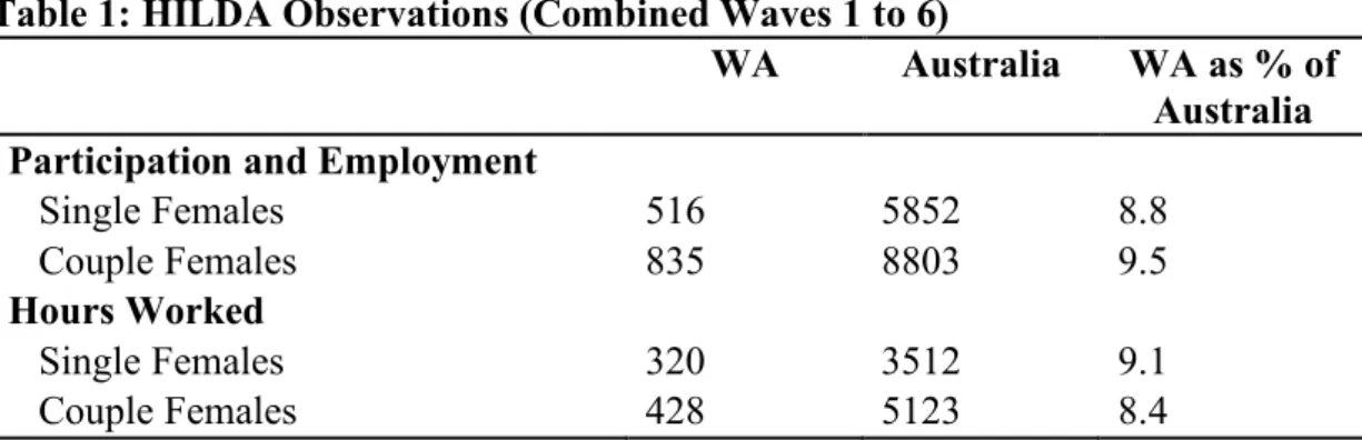
There are 21688 usable observations from waves 1 to 6 of the HILDA for Australia and 2172 for Western Australia which result in 1351 and 14655 usable observations for females for WA and Australia respectively. From this sample, 1351 (WA) and 14655 (Australia) females are labour force participants, and 748 (WA) and 8635 (Australia) females supply hours of labour (see Table 1 below).

Table 1: HILDA Observations (Combined Waves 1 to 6)

WA Australia WA as % of Australia Participation and Employment

Single Females 516 5852 8.8

Couple Females 835 8803 9.5

Hours Worked

Single Females 320 3512 9.1

Couple Females 428 5123 8.4

Notes: (1) Sample HILDA pooled data Wave 1 to 6 (unweighted). (2) Sample is unbalanced (individuals need not be present for all waves)—there are an average of approximately 2.5 observations for each individual (with a range of 1 to 6 waves of observations).

Sample Size and Statistical Significance

From Table 1 above it is apparent that there are important differences in sample size: the sample sizes for WA are small in comparison with the sample size for Australia—for example, in the sample used to estimate labour force participation for single females, there are 516 observations (216 individuals) in WA, compared to 5852 observations (2340 individuals) for Australia. In addition, the WA sample is small in comparison with the usual

11_{It is common in labour market studies to restrict analysis to this age group (although the sample can be} restricted to those under, say, 55 if it is thought that the behaviour of those nearing retirement will differ from the younger individuals).

(13)

sample size encountered, and preferred, in empirical research directed at labour market issues. Thus, for example, most Australian studies focus on the national population.

Rules-of-thumb have been suggested for determining the minimum sample size for multiple regression analyses (Tabachnick and Fidell 1996). Simple rules such as a ratio of 5 to 1 for observations and explanatory variables (e.g. Hair Jr et al. 1992) are generally considered too simplistic; Green (1991) provides some support for the general rule that N ! 50 + 8K is sufficient (where N represents the minimum sample size and K the number of explanatory variables in the regression model), while Montenegro (2001) provides support for the simple rule N = 10K. More complex sample size determination methods do not appear to provide sufficient advance: there is a tendency to trade simplicity for absolute accuracy when determining minimum sample size (Green 1991). It is clear that for models for WA for labour market outcome, the sample size boarders on being “too small”—estimated coefficients and their standard errors will show little or no bias (Maas and Hox 2004), but statistical tests (e.g. the t-statistic for individual coefficients) which rely on sample size for precision will be unreliable. Thus, interpreting the statistical significance—and hence implications for individual behaviour—must be done with care for econometric models based on small samples (and to a lesser extent, very large samples).

To reduce the potential for large sample results leading to statistical significance when only small differences are “detected”, the usual 5% level (p-value ! 0.05) of statistical significance is maintained as the necessary (maximum) level for models based on the sample for Australia; to reduce the potential that for small sample models for WA the probability of “correctly” finding statistical significance is reduced, in the model results considered below, statistical significance at the 10% level (p-value ! 0.10) is treated as acceptable (Leamer 1978; Kennedy 1998).12

Given the issues regarding small and large samples, and that the aim of this Report is to provide distinct analysis for WA, it must be recognised that, to the extent Australia and WA are similar, models for Australia are likely to be a superior guide as to underlying drives of labour market behaviour and to provide implications for policy directions. Throughout this Report, generally, both the Australia and WA results are discussed as they provide insights into participation and hours worked—and they suggest further avenues for research. Nonetheless, unless the WA government funds a larger sample survey for WA, the problems of sample size are going to remain in all further work relating specifically to WA; that is, statistical significance (indicating an explanatory variable is relevant) will be harder to discover and model results will remain less reliable than studies based on the complete HILDA data set.

In the next section, issues relating to appropriate model building for panel data based on restricted samples are considered.

12_{Statistical significance is a function of sample size. The (two-sided}_t_{-statistic) test for the significance of} individual coefficients is Ho:" = 0 vs. the alternative Ha:"# 0, where the test statistic is calculated as Coefficient/Standard Error = "/SE (and the standard error is calculated as Standard Deviation/$Sample Size=SD/$N hence the t-statistic is calculated as "/(SD/$N) so as the sample size gets smaller the t-statistic is less likely to be statistically significant. Thus, for very large samples, small differences may be ‘detected’ as significant, but for very small samples the probability of finding statistical significance is reduced.

(14)

Econometric Issues for Model Building

The panel data econometric models in this Report deal with two issues pertaining to females in WA: the supply of hours (the Hours equation, contingent on the probability of being employed) and the decision to participate in the labour force. For convenience in discussing the rational for the econometric models, the Hours equation (including the influence of the probability of being Employed equation) is considered first—the probability of being a labour force participant (the Participation) equation can then be presented simply as a parallel to the employment equation (i.e. both are limited dependent variable specifications). Before outlining the specific models used in this Report it is necessary to deal with two complexities for econometric modelling:

a) Sample selection bias—present when the sub-sample being analysed (e.g. those who supply hours of work) is a non-random selection from a larger sample (e.g. all employed female labour force participants in the specified age group).

b) Panel versus cross-sectional econometric modelling—the benefits and drawbacks of using sophisticated (and more complex) panel data models versus the more common and less sophisticated cross-sectional models.

Sample Selection Bias

Sample selection bias occurs naturally in labour supply modelling as hours worked (or wage rates) and the probability of being employed (or of being a labour force participant) are inter-related.13 Potential bias arises from the exclusion of non-working females from the sample when estimating the hours of work equation). As the hours worked of non-working females are zero, the distribution of hours is truncated. Thus, the sample of those who do supply hours overstates the desire to supply hours of work beyond that of the population of all females of the selected age range). In the econometric model that do not account for this “selection bias” the error term will not necessarily be a mean-zero random variable in the resulting sub-sample of women who supply hours of work (it generally tends to be positive) even though it is a mean-zero random variable in the population of all females. Consequently, econometric model-based estimates of coefficients may be biased and inconsistent (i.e. amongst other things, the size and statistical significance of individual model estimates or coefficients may lead to false conclusions and poor policy prescription or advice).

Since Heckman (1978, 1979), it has been commonplace in econometric analysis to correct for sample selection bias when estimating labour supply models through a two-step procedure. In the first step, a “reduced form” secondary equation is specified: for example, when modelling wage outcomes, a probability of Participation in the labour force equation is fitted for the complete random sample. Outcomes from the Participation equation are then used to construct a selection bias “correction term” that is incorporated into the second step “structural” or primary wage equation and by accounting for the non-randomness of the sample for wage earners (a non-random sub-sample of all surveyed individuals) controls for selection bias. If the model is to explain hours of labour supply (an Hours equation) sample selection is due to the sample of those supplying hours of work being a non-random sub-set of all individuals.

13_{More specifically, the dependent variable hours, to be explained by regression analysis, is non-randomly} selected because the probability of being employed influences the number of hours worked.

(15)

Despite the achievements of the Heckman two-step procedure in overcoming sample selection bias, its application in empirical studies has been limited to cross-sectional data (or pooled panel data) analysis (see below). It is only recently that well developed two-step panel data procedures, similar to the Heckman two-step cross-sectional procedure, have been developed (based on innovative work by Ridder (1990); Nijman and Verbeek (1992); and Vella and Verbeek (1999). The advanced two-step estimation procedure developed by Vella and Verbeek (1999) is adopted in this Report to estimate labour supply models (see below).

Cross-Sectional versus Panel Data Econometric Analysis

As is well documented, the consequence of using cross-sectional (or pooled panel data) is that individuals’ unobserved time-constant characteristics (or unobserved heterogeneity14_{) are} not considered; unobserved heterogeneity, if present, results in inefficient econometric model estimates (with high standard errors leading to lack of statistical significance of estimated parameters). Moreover, treating panel or longitudinal data as if it were a cross-section ignores the information contained in the progress or change in measured variables, and importantly ignores that in panel data across-time correlations are common; autocorrelation results in inefficient parameter estimates, standard errors of the estimates are biased invalidating hypothesis tests such as t-statistics, and the R2 (coefficient of determination15) is no longer reliable (Greene 2003). Moreover, the scarcity of Australian longitudinal survey data incorporating “economic”, has until recently contributed to the restriction to analysis at the cross-sectional data level. The HILDA survey data has provided much needed longitudinal data for Australia. Nonetheless, as discussed in detail above, the availability of HILDA data may not have solved the problem for analysis at the Australian state level as sample size for smaller population states remains small.

Panel data models treat the unobserved heterogeneity as a random variable: alternative assumptions are that the heterogeneity is not correlated with the (exogenous) explanatory variables (the random effects model, REM) or that there is correlation (the fixed effects model, FEM).16 There are benefits and drawbacks of both approaches to panel data modelling—subject to much discussion in the econometric literature (see e.g. Lester, 2007 for a review). Despite the advances in panel data analysis, there are few estimators for panel models with limited dependent variables and sample selection, but the Vella and Verbeek (1999) two-step procedure deals with these mattes. Moreover, the method allows the inclusion in the econometric model specification of explanatory variables that may be correlated with the unobserved heterogeneity, and of time-invariant (or slow-changing) explanatory variables that are not usual in FEM models.17

Having dealt with issues common to panel data analysis and sample selection an overview of the current state of knowledge regarding labour market supply by individuals and couples follows.

14_{Note that the unobserved heterogeneity is not itself of interest in the analysis: interest is in controlling for the} potential bias caused by ignoring its influence.

15_{A measure of model goodness-of-fit bounded between zero and one, where R}2 _{= 1 represents a perfect fit.} 16_{Notwithstanding the confusion that may be created by the nonclamature REM and FEM, in both cases the} individual unobserved heterogeneity is assumed to be a random variable. In the FEM model, heterogeneity is treated as an (estimateable) individual specific dummy variable (generally resulting in the incidental parameter problem) but in the REM, individual unobserved heterogeneity is assumed to have an empirical distribution. 17_{Since the FEM model is based on first-differences (e.g. xit-xit-1) time-invariant explanatory variables are} “differenced” out of the models.

(16)

Unitary and Collective Models of Labour Supply

In the analysis presented in this Report, household labour supply is estimated based on the “unitary” labour supply model. Although, as outlined below, the more recent literature suggests a “collective” model of household labour supply is more appropriate for households with two (or more) adults, currently available econometric software precludes the use of the more advanced estimators.

It is commonplace in microeconomic analysis to treat household labour supply behaviour as the utility maximisation behaviour of an individual (i.e. the household is treated as if it were an individual)—referred to in the literature as the “unitary” labour supply approach. In recent years, however, the unitary approach has been criticised at the theoretical level because it assumes that the household is characterised by a single preference or utility function. In the common unitary model, a couple in a household are treated as if they are a single unit—or, as if one individual made all the decisions concerning the labour supply provision of all household members to maximise joint utility. Hence, the unitary model approach does not allow individual household members’ preferences to be considered, or the intra-household distribution of welfare to be identified. In Addition, the unitary model implies that household members aggregate, or pool, their incomes so that labour supply and consumption decisions are determined only by the total exogenous income (which may include welfare payments and investment income), rather than the distribution of income across household members. Modelling labour supply of households that includes two or more income earners (such as couple households), by application of the unitary model has come under much scrutiny both theoretically and empirically recently, and in general, the theoretical restrictions that the unitary model approach imposes are not necessarily supported by the empirical literature for households that contain more than one individual. The result of the recent evaluation of the unitary model has been the development of the “collective” approach, which considers the household members individual, but interrelated, labour supply behaviour rather than the household as if it were a single unit (Chiappori 1988; 1992).

The collective approach explicitly determines household labour supply and consumption decisions by means of the individual household members’ preferences or utility functions— which allow the inclusion of the partner’s welfare to be taken. In the Chiappori (1988; 1992) approach, when the preferences of one or more individuals in a couple household include concern for their own welfare and the welfare of their partner,18 then a bargaining process dictates labour supply. Thus, in the collective model of labour supply for partner households, the interaction between household members’ labour supply decisions is explicitly recognised through a sharing rule based on the division of household income between the partners. The welfare function defined in the collective model can be interpreted as a method which defines an inter-household bargaining process. Labour supply is a two-stage process, first non-labour income—a function of wage rates—is divided between individual household members, and in the second-stage individuals decide about their labour supply conditional on their share on non-labour income.19

18_A_{nd, their consumption is private—e.g. individuals do not share the consumption of goods such as clothes.} 19 _{A useful explanation of the assumption underpinning the bargaining process between the individuals in a} household is explained by application of economic Game theory which show how the economically efficient (Nash equilibrium) can be obtained (Ligon 2002; Chiappori and Donni 2005).

(17)

An extensive review of the econometric literature, however, indicates that the application of the two-step panel model has limitations. Thus, a comprehensive model of female labour supply (hours of work) would include both single and partnered individuals, with or without children, who do or do not participate in the labour force, which includes individual utility functions for partnered households and the rules or process for joint decisions about the supply of labour hours by each household member. At the current stage of development, however, this comprehensive, inclusive, panel data model is not available. The application of the collective approach to couple households that contain children (who, in the collective model, must be treated as a public good) are still in their infancy, as are models which include non-participants—with many models restricted to households without children where the couple are both employed (Donni 2003; Bloemen 2004; Blundell et al. 2007; Couprie 2007; Van Klaveren 2008).

Although variations on the collective model can be written in equation form, no theoretical microeconometric solution has yet been devised, and hence software to estimate the model has not been written (i.e. accessible econometrics packages do not include an appropriate econometric estimator for the collective models). Currently, restrictive estimators devised that provide accessible econometric models for simplified models only. The Vella and Verbeek (1999) model, which can be applied to single and couple females separately represents the current level of sophistication available for applied econometric panel data models of labour supply, but its theoretical base is the unitary model. Consequently, the unitary approach has been adopted in this Report for analysis of couple households with and without children. Future research should be considered to overcome this simplification, and potential mis-specification when applying the unitary model to couples.

Simultaneity and the Two-Step Selection Bias Model

s

The collective model outlined above does not require a simultaneous equation model of female and male behaviour for couple households because the interaction is accommodated through the bargaining process—hours of labour supply are an inter-related decision of household members. In the unitary model of labour supply, one approach is to consider a simultaneous equation model for individual female and male supply in which partner’s wage and hours of work (or wage per hour) appear in the hours supplied equation. The drawback of this approach (abstracting from the preference for a collective model) is that wage and hours on the right-side of equations are endogenous (they are simultaneously determined). Consequently, an instrumental variables (IV) model is required. As with all IV models, it is not clear which instruments are appropriate, and there is the persistent difficulty of finding instruments that correlate with the endogenous variable but are suitable exogenous. Further, the current specification of the two-step selection bias model does not accommodate a simultaneous equation model of female and male behaviour for couple households. The approach adopted in this Report is to include a number of male partner characteristics which attempts to capture the “flavour” of joint decision-making to some extent, while avoiding practical and econometric problems such as the IV approach.

The following section describes the process of applying theoretical labour supply models to observed data. Models are presented in a simplified form (for a more technically detailed expose see Vella and Verbeek 1999).

(18)

The Two-step Econometric Model of Hours of Work Supplied

Having discussed the underlying theoretical implications of estimating a labour supply model, the specification of the econometric models are considered. In this Report, the estimation of the labour supply model follows closely the two-step panel data procedure developed by Vella & Verbeek (1999) to overcome selection bias and endogeneity in the labour supply equation.

In the Vella and Verbeek (1999) model approach, the estimates of a “structural” primary hours worked equation [1], are obtained via a “reduced form” secondary equation [2] which determines the selection rule—the probability of being employed. Equation [3] determines when the probability of being employed is positive. Equation [4] determines (based on selection equation [3]) when labour hours supply is greater than zero—Equations [3] and [4] are referred to as the censoring and selection rules.

Two-Step Panel Data Model

Primary “Structural” Hours Supplied Equation:

(

)

1 , ; 1

it it it i it

Hours# f

x

Employed ! µ "

= + + [1]

Secondary “Reduced Form” Employment Equation:

(

)

2 , , 1; 2

it it i t i it

Employed$ = f

x

Employed % ! +" +# [2]

Censoring and Selection Rules

Probability of Being Employed Equation:

(

)

3 ; 3

it it

Employed f Employed" !

= [3]

Hours Supplied Equation:

it it

Hours Hours!

= if f Employed4

(

i1, ,K EmployediT

)

=1 0

it

Hours = if f Employed4

(

i1, ,K EmployediT

)

=0 [4]

where i are individuals (survey participants, i = 1,…, N), t is time (or survey waves,

t = 1,…, T), and f represents functions characterised by the unknown parameters (vector) ". The

x are the vector of observed individual characteristics or explanatory variables (e.g.

education level, children in the household, marital status, partner’s attributes, etc.), and covariates or control variables which while influential are not the subject of interest in this Report. Random, time-invariant, individual heterogeneity are represented by µi and "i and random, time-variant, individual specific, independent, effects as %it and #it. Note that x need not contain identical explanatory variables across functions. Starred variables are latent (unobserved) endogenous variables (i.e. preferred hours supplied, Hours*, and the probability of a labour force participant being employed, Employed*)—with observed counterparts (actual hours supplied, Hours; and whether or not employed, Employed). The terms µi and "i represent the panel-model (random) time-invariant unobserved individual effects (heterogeneity), and %it and &it represent the random individual-specific time-variant effects— that are assumed independent across individuals.

(19)

To specify the “correction” terms estimated in Equation [1] to be incorporated into Equation [2], allow the error component of the secondary equations (e.g. the reduced form probability of employment) to be denoted by uit = "i + $it (i.e., a combination of individual time-invariant unobserved heterogeneity and an individual time-varying component). The time-invariant “correction” is approximated by the mean of the time-varying component, ui (i.e. the average of the uit20), and the time-varying correction is uit. Thus, in the Hours equation, the panel-model unobserved heterogeneity (µi) and time-variant heterogeneity (%it) are approximated by

i

u and uit respectively; as ui and uit are treated as “data” in the Hours equation, their parameters (coefficients) can be estimated and if non-significant suggest no endogeneity. The model of Equations [1] to [4] demonstrates that the determination of Employed (the probability of employment) is a function (f3) of the unknown parameter vector "3, and the function f4 indicates that Hours (actual worked) is only observed for positive values of

Employed. Thus, sample selection bias in the primary Hours equation is controlled for by including the selection and censoring rule from the Employed equation (Employmentit)—the primary Hours equation should not be estimated without first considering what determined its sub-sample, the reduced form Employed equation, or parameter estimates are potentially biased and inconsistent leading to incorrect attribution of causes of hours supplied.

Thus, the two-step model depicted above describes how to control or account for selection bias, and the inclusion of individual effects controls for heterogeneity in the panel data econometric models.

For estimation, further assumptions are made: as usual, errors are normally distributed and explanatory variables are exogenous; autocorrelation in the secondary reduced form

Employed probit equation errors is inadmissible, but heteroscedasticity and/or autocorrelation in the primary Hours equation errors can be accommodated.

As shown in the reduced form Equation [2], the model features a potential role for dynamics (e.g. Employmenti,t-1): in addition, “state dependence” is controlled by inclusion of information on the dependent variable in the period preceding the first available data period (Employmenti,t=0).21 The inclusion of Employmentt=0 may be endogenous due to recall problems or respondents’ perceptions when concurrently reporting their current and previous behaviour at t = 1. The example provided by Vella and Verbeek (1999) found that while endogeneity existed, it did not affect the results in any significant way, nonetheless, they suggest potential endogeneity (due to dynamics and/or state dependency) can be controlled by including a polynomial of predicted values of the dependent variable from the Employed

equation including in the Hours equation.

For the purposes of this Report, the lagged dependent variable for the zero period was constructed using information provided by respondents in the first time period above their experience in the previous year,22 which controls for “state dependency” (and has the benefit of preserving observations—particularly important for the relatively small samples for WA). Potential endogeneity was controlled by the Employed polynomial (in addition to the selection bias and heterogeneity correction terms in the Hours equation).

20_{More generally,} 1 1 W i i t it u W! u =

= " where Wi represents the number of waves for individual i. 21_{In model estimation, a single variable includes both}_Employment

i,t-1 and Employmenti,t=0. 22_{When new households form, period “zero” (the previous year) may be between waves 1 and 5.}

(20)

Empirical Equations for the Two-step Model of Hours Worked

Based on the theoretical model outlined above, the empirical equations can be specified. First, Employed is estimated as a limited dependent variable (probit) panel data model (see Appendix I for the probit model specification). Second, Hours is estimated as a panel data model of a continuous dependent variable, corrected for selection bias (i.e. only employed labour force participants supply hours worked) by inclusion of panel data “correction” terms (the ui and uit “data”):

1 1, ... , , 1 it it k k it E i t i it Employed$ ! x ! x ! Employment " # % = + + + + + [5]

(

)

1 1, ... , ; it it k k it P it P i it Hours =! x + +! x + f Employment ! +u +u [6]

Where the quadratic function (fP) to control for endogeneity is defined as:

(

)

2 1 2 3 4 3 4 ; P it P P it P it P it P it

f Employed Employment Employment

Employment Employment

! ! !

! !

= +

+ + [7]

where Hours represents the log of hours worked in paid employment per week,

x represent

observed independent or explanatory variables (e.g. work experience, education, health, and marital status). fP denotes a polynomial (of pre-specified length) with unknown coefficients ("P) controlling for endogeneity due to dynamics, and "E controls for “state dependence”. Note that the Employed equation is required in contrast to a Participation equation because the selection bias is due to selection into employment not selection into participation—hours supplied are not independent of selection into employment—a female who is not employed does not independently select her hours of work.

The Participation Equation

The participation equation, modelled as a panel data limited dependent variable probit model has the following specification:

1 1, ... , , 1 it it k k it P i t i it Participation$ ! x ! x ! Participation " # % = + + + + + [8] Where: 0 it

Participation = if f ParticipationP( it,....,ParticipationiT) 0

! ! = it it Participation Participation! = if f ParticipationP( it,....,ParticipationiT) 1 ! ! = [9] where Participation* represent the (unobserved) endogenous probability of being a labour force participant—with observed counterpart Participation. As previously,

x represent

observed independent or explanatory variables, Participationi,t-1 controls for “state dependency”, "s are parameters to be estimated, "i represent the unobserved individual unobserved random effects (heterogeneity), and &it are the usual regression error terms. As it is hours supplied and participation that are the primary concern of this Report, estimates relating to these two functions are summarised and discussed below (since the employment equation is included to control for selection bias the results are not discussed)—full

(21)

econometric output from models for the probability of participating in the labour market, the probability of being employment, and hours of labour supply is provided in Appendix II.

Summary Statistics

Table 2 provides a legend of variable names and description of those included in models for WA and Australia, and Table 3, which follows, has summary statistics for these variables.

Table 2: Legend: Explanatory Variables Used in Econometric Models

Variable Name Description Variables Required

lnhoursf Log of weekly hours worked in paid employment Continuous

lbfst & lbfst_lag Employed (full-time or part-time) and unemployed or not

in the labour force (and the one-period lag)

Binary state

exp Total employment experience in years Continuous

exp-sq Total employment experience in years squared Continuous

jbsearch Total time out of employment in years Continuous

jbsearch_sq Total time out of employment in years squared Continuous

ed1

Highest level of education is Bachelor/Graduate

Diploma/Postgraduate degree Dummy

ed2

Highest level of education is Advanced Diploma/Diploma

Dummy

ed3 Highest level of education is Certificate III/IV Dummy

ed4 Highest level of education is Certificate I/II or Year 12 Dummy

ed5 (base)

Highest level of education is Year 11 & below, or undetermined

Dummy ped1

Partner’s highest level of education is Bachelor/Graduate Diploma/Postgraduate degree

Dummy ped2

Partner’s highest level of education is Advanced Diploma/Diploma

Dummy

ped3 Partner’s highest level of education is Certificate III/IV Dummy

ped4

Partner’s highest level of education is Certificate I/II or Year 12

Dummy

ped5 (base) Partner’s highest level of education is Year 11 & below Dummy

C4_1 One resident child under 5 years, and no others Dummy

C4_2 2 or more resident children under 5 years, and no others Dummy

C514_1 One resident child between 5-14 years, and no other Dummy

C514_2 2 or more resident children age 5-14 years, and no others Dummy

C4 Any resident children between 0-4 years, and no others Dummy

nonresch Any non-resident children Dummy

pnonresch Partner has any non-resident children Dummy

wage Real hourly wage of female (AUD)* _Continuous

wage_sq Real hourly wage of female squared (AUD)* Continuous

pwage Real hourly wage of male partner (AUD)* _Continuous

nonlbinc Real non-labour income^ Continuous

rural Household located in a rural area# Dummy

age Age of females (between 18 and 64 years) Continuous

age_sq Age of females squared Continuous

An Econometric Evaluation of Women s Labour Supply in WA

An Econometric Evaluation of

Women’s Labour Supply in WA

A Report Prepared for the Western

Australia Department of Consumer

and Employment Protection

Laurence Lester and Darcy Fitzpatrick

23 July 2008

An Econometric Evaluation of Women’s Labour Supply in WA

A Report Prepared for the Western Australia Department of

Consumer and Employment Protection

Laurence Lester and Darcy Fitzpatrick

National Institute of Labour Studies

23 July 2008

Contents

List of Tables

Executive Summary

Female Labour Force Participation

Supply of Hours of Paid Work

Conclusion

Suggestions for further Research

The Work Undertaken

Background

Labour Supply Shortages—WA and Australia

Employment Issues

Focus of Attention in this Report

Factors Influencing Women’s Labour Supply

x

The HILDA Data

Econometric Issues for Model Building

Sample Selection Bias

Cross-Sectional versus Panel Data Econometric Analysis

Unitary and Collective Models of Labour Supply

Simultaneity and the Two-Step Selection Bias Model

s

The Two-step Econometric Model of Hours of Work Supplied

(

)

x

(

)

x

(

)

(

)

(

)

x are the vector of observed individual characteristics or explanatory variables (e.g.

Empirical Equations for the Two-step Model of Hours Worked

(

)

(

)

x represent

The Participation Equation

x represent

Summary Statistics