Web Data Indexing in the Cloud:
Efficiency and Cost Reductions
Jesús Camacho-Rodríguez
Dario Colazzo
Ioana Manolescu
OAK team, Inria Saclay and LRI, Université Paris-Sud
[email protected]
ABSTRACT
An increasing part of the world’s data is either shared through the Web or directly produced through and for Web plat-forms, in particular using structured formats like XML or JSON. Cloud platforms are interesting candidates to handle large data repositories, due to their elastic scaling proper-ties. Popular commercial clouds provide a variety of sub-systems and primitives for storing data in specific formats (files, key-value pairs etc.) as well as dedicated sub-systems for running and coordinating execution within the cloud.
We propose an architecture for warehousing large-scale Web data, in particular XML, in a commercial cloud plat-form, specifically, Amazon Web Services. Since cloud users support monetary costs directly connected to their consump-tion of cloud resources, we focus on indexing content in the cloud. We study the applicability of several indexing strate-gies, and show that they lead not only to reducing query evaluation time, but also, importantly, to reducing the mon-etary costs associated with the exploitation of the cloud-based warehouse. Our architecture can be easily adapted to similar cloud-based complex data warehousing settings, car-rying over the benefits of access path selection in the cloud.
Categories and Subject Descriptors
H.2.4 [Database Management]: Systems—Concurrency, Distributed databases, Query processing
General Terms
Design, Performance, Economics, Experimentation
Keywords
Cloud Computing, Web Data Management, Query Process-ing, Monetary Cost
1.
INTRODUCTION
An increasing part of the world’s interesting data is either shared through the Web, or directly produced through and for Web platforms, using formats like XML or more recently JSON. Data-rich Web sites such as product catalogs, social media sites, RSS and tweets, blogs or online publications ex-emplify this trend. By today, many organizations recognize the value of the trove of Web data and the need for scalable platforms to manage it.
Simultaneously, the recent development of cloud comput-ing environments has strongly impacted research and
devel-c
ACM, 2013. This is the author’s version of the work. It is posted here by permission of ACM for your personal use. Not for redistribution. The definitive version was published in EDBT’13, March 18–22, 2013, Genoa, Italy.http://doi.acm.org/10.1145/2452376.2452382.
opment in distributed software platforms. From a business perspective, cloud-based platforms release the application owner from the burden of administering the hardware, by providing resilience to failures as well as elastic scaling up and down of resources according to the demand. From a (data management) research perspective, the cloud provides a distributed, shared-nothing infrastructure for data storage and processing.
Over the last few years, big IT companies such as Amazon, Google or Microsoft have started providing an increasing number of cloud services built on top of their infrastructure. Using these commercial cloud platforms, organizations and individuals can take advantage of a deployed infrastructure and build their applications on top of it. An important fea-ture of such platforms is their elasticity, i.e., the ability to allocate more (or less) computing power, storage, or other services, as the application demands grow or shrink. Cloud services are rented out based on specific service-level agree-ments (SLAs) characterizing their performance, reliability etc.
Although the services offered by public clouds vary, they all provide some form of scalable, durable, highly-available store for files, or (equivalently) binary large objects. Cloud platforms also provide virtual machines (typically called in-stances) which are started and shut down as needed, and on which one can actually deploy code to be run. This gives a basic roadmap for warehousing large volumes of Web data in the cloud in a Software-as-a-Service (SaaS) mode: to store the data, load it in the cloud-based file store; to process a query, deploy some instances, have them read data from the file store, compute query results and return them.
Clearly, the performance (response time) incurred by this processing is of importance; however, so are the monetary costs associated to this scenario, that is, the costs to load, store, and process the data for query answering. The costs billed by the cloud provider, in turn, are related to the total effort (or total work), in other terms, the total consumption of all the cloud resources, entailed by storage and query processing. In particular, when the warehouse is large, if query evaluation involves all (or a large share of) the data, this leads to high costs for: (i) reading the data from the file store and (ii) process the query on the data.
In this work, we investigate the usage of content indexing, as a tool to both improve query performance, and reduce the total costs of exploiting a warehouse of Web data within the cloud. We focus on tree-structured data, and in par-ticular XML, due to the large adoption of this and other tree-shaped formats such as JSON, and we considered the
particular example of the Amazon Web Services (AWS, in short) platform, among the most widely adopted, and also target of previous research works [6, 23]. Since there is a strong similarity among commercial cloud platforms, our re-sults could easily carry on to another platform (we briefly discuss this in Section 3). The contribution of this work are:
• A generic architecture for large-scale warehousing of complex semistructured data (in particular, tree-shaped data) in the cloud. Our focus is on building and ex-ploiting an index to simultaneously speed up process-ing and reduce cloud resource consumption (and thus, warehouse operating costs);
• A concrete implemented platform following this archi-tecture, demonstrating its practical interest and val-idating the claimed benefits of our indexes through experiments on a 40 GB dataset. We show that in-dexing can reduce processing time by up to two orders of magnitude and costs by one order of magnitude; moreover, index creation costs amortize very quickly as more queries are run.
Our work is among few to focus on cloud-based index-ing for complex data; a preliminary version appeared in [8], and an integrated system based on the work described here was demonstrated in [4]. Among other previous works, our work can be seen as a continuation of [6, 19], which also exploited commercial clouds for fine-granularity data man-agement, but (i) for relational data, (ii) with a stronger fo-cus on transactions, and (ii) prior to the very efficient key-value stores we used to build indexes reducing both costs and query evaluation times.
The remainder of this paper is organized as follows. Sec-tion 2 discusses related works. SecSec-tion 3 describes our archi-tecture. Section 4 presents our query language, while Sec-tion 5 focuses on cloud-based indexing strategies. SecSec-tion 6 details our system implementation on top of AWS, while tion 7 introduces its associated monetary cost model. Sec-tion 8 provides our experimental evaluaSec-tion results. We then conclude and outline future directions.
2.
RELATED WORK
To the best of our knowledge, distributed XML indexing and query processing directly based on commercial cloud ser-vices had not been attempted elsewhere, with the exception of our already mentioned preliminary work [8]. That work presented index-based querying strategies together with a first implementation on top of AWS, and focused on tech-niques to overcome Amazon SimpleDB1limitations for man-aging indexes. This paper features several important nov-elties. First, it presents an implementation which relies on Amazon’s new key-value store, DynamoDB, in order to en-sure better performance in managing indexes, and, quite im-portantly, more predictable monetary cost estimation. We provide a performance comparison between both services in Section 8. Second, it presents a proper monetary cost model, which still remains valid in the contexts of several alterna-tive commercial cloud services. Third, it introduces multiple optimizations in the indexing strategies. Finally, it reports about extensive experiments on a large dataset, with a par-ticular focus on performances in terms of monetary cost. 1
http://aws.amazon.com/simpledb/
Alternative approaches which may permit to attain the same global goal of managing XML in the cloud comprises commercial database products, such as Oracle Database, IBM DB2 and Microsoft SQL Server. These products have included XML storage and query processing capabilities in their relational databases over the last ten years, and then have ported their servers to cloud-based architectures [5]. Differently from our framework, such systems have many functionalities beyond those for XML stores, and require non-negligible efforts for their administration, since they are characterized by complex architectures.
Recently, a Hadoop-based architecture for processing mul-tiple twig-patterns on a very large XML document has been proposed [10]. This system adopts static document parti-tioning; the input document is statically partitioned into several blocs before query processing, and some path mation is added to blocs to avoid loss of structural infor-mation. Also, the system is able to deal with a fragment of XPath 1.0, and assumes the query workload to be known in advance, so that a particular query-index can be built and initially sent to mappers to start XML matching. Differ-ently, in our system we do not adopt document partition-ing, the query workload is dynamic (indexes only depends on data) and, importantly, we propose a model for monetary cost estimation.
Another related approach is to aim at leveraging large-scale distributed infrastructures (e.g., clouds) by intra-query parallelism, as in [11], enabling parallelism in the processing of each query, by exploiting multiple machines. Differently, in our work, we consider the evaluation of one query as an atomic (inseparable) unit of processing, and focus on the horizontal scaling of the overall indexing and query process-ing pipeline distributed over the cloud.
The greater problem of distributed XML data manage-ment has been previously addressed from many other angles. For instance, issues related to XML data management in clusters were largely studied within the Xyleme project [1]. Further, XML data management in P2P systems has been a topic of extensive research from the early 2000’s [18].
Finally, some recent works related to cloud services have put special emphasis on the economic side of the cloud. For instance, the cost of multiple architectures for transaction processing on top of different commercial cloud providers is studied in [19]. In this case, the authors focus on read and update workloads rather than XML processing, as in our study. On the other hand, some works have proposed mod-els for determining the optimal price [14] or have studied cost amortization [15] for data-based cloud services. How-ever, in these works, the monetary costs are studied from the perspective of the cloud providers, rather than from the user perspective, as in our work.
3.
ARCHITECTURE
We now describe our proposed architecture for Web data warehousing. To build a scalable, inexpensive data store, we store documents as files within Amazon’s Simple Stor-age Service (S3, in short). To host the index, we have dif-ferent requirements: fine-grained access, and fast look-up. Thus, we rely on Amazon’s DynamoDB efficient key-value store for storing and exploiting the index. Within AWS, in-stances can be deployed through the Elastic Compute Cloud service (EC2, in short). We deploy EC2 instances to (i) ex-tract from the loaded data index entries, and send them to
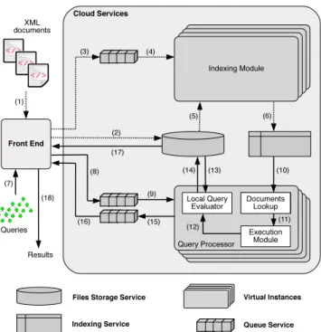
Figure 1: Architecture overview.
Dynamo DB’s index and (ii) evaluate queries on those sub-sets of the database resulting from the query-driven index lookups. Finally, we rely on Amazon Simple Queue Ser-vice (SQS, in short) asynchronous queues to provide reliable communication between the different modules of the appli-cation. Figure 1 depicts this architecture.
User interaction with the system involves the following steps. When a document arrives (1), the front end of our application stores it in the file storage service (2). Then, the front end module creates a message containing the ref-erence to the document and inserts it into theloader request
queue (3). Such messages are retrieved by any of the virtual machines running our indexing module (4). When a message is retrieved, the application loads the document referenced by the message from the file store (5) and creates the index data that is finally inserted into the index store (6).
When a query arrives (7), a message containing the query is created and inserted into the query request queue (8). Such messages are retrieved by any of the virtual instances running our query processor module (9). The index data is then extracted from the index store (10). Index storage services provide an API with rather simple functionalities typical of key-value stores, such as get and put requests. Thus, any other processing steps needed on the data re-trieved from the index are performed by a standard XML querying engine (11), providing value- and structural joins, selections, projections etc.
After the document references have been extracted from the index, the local query evaluator receives this informa-tion (12) and the XML documents cited are retrieved from the file store (13). Our framework includes “standard” XML query evaluation, i.e. the capability of evaluating a given queryq over a given documentd. This is done by means of a single-site XML processor, which one can choose freely. Thus, the virtual instance runs the query processor over the documents and extracts the results for the query.
Finally, we write the results obtained in the file store (14) and we create a message with the reference to those results
Provider File store Key-value store Computing Queues Amazon Web Services Amazon Simple Storage Service Amazon DynamoDB, Amazon SimpleDB Amazon Elastic Cloud Compute Amazon Simple Queue Service Google Cloud Google Cloud Storage Google High Replication Datastore Google Compute Engine Google Task Queues Windows Azure Windows Azure BLOB Storage Windows Azure Tables Windows Azure Virtual Machines Windows Azure Queues
Table 1: Component services from major commer-cial cloud platforms.
q1 painting nameval painter nameval q2 painting descriptioncont year=1854 q3 painting
namecontains(Lion) painter
name lastval q4 painting nameval painter name last=Manet year1854<val≤1865 q5 museum nameval painting @id painting @id painter name last=Delacroix
Figure 2: Sample queries.
and insert it into the query response queue (15). When the message is read by the front end (16), the results are retrieved from the file store (17) and returned (18).
Scalability, parallelism and fault-tolerance. The
ar-chitecture described above exploits the elastic scaling of the cloud, for instance increasing and decreasing the number of virtual machines running each module. The synchronization through the message queues among modules provides inter-machine parallelism, whereas intra-inter-machine parallelism is supported by multi-threading our code. We have also taken advantage of the primitives provided by message queues, in order to make our code resilient to a possible virtual in-stance crash: if an inin-stance fails to renew its lease on the message which had caused a task to start, the message be-comes available again and another virtual instance will take over the job.
Applicability to other cloud platforms. While we have
instantiated the above architecture based on AWS, it can be easily ported to other well-known commercial clouds, since their services ranges are quite similar. Table 1 shows the ser-vices available in the Google and Microsoft cloud platforms, corresponding to the ones we use from AWS.
4.
QUERY LANGUAGE
We consider queries are formulated in an expressive frag-ment of XQuery, amounting to value joins over tree patterns. For illustration, Figure 2 depicts some queries in a graphical notation which is easier to read. The translation to XQuery
syntax is pretty straightforward and we omit it; examples, as well as the formal pattern semantics, can be found in [21]. In a tree pattern, each node is labeled either with an XML element or attribute name. By convention, attribute names are prefixed with the@sign. Parent-child relationships are represented by single lines while ancestor-descendant rela-tionships are encoded by double lines.
Each node corresponding to an XML element may be an-notated with zero or more among the labels val andcont, denoting, respectively, whether the string value of the ele-ment (obtained by concatenating all its text descendants) or the full XML subtree rooted at this node is needed. We support these different levels of information for the following reasons. The value of a node is used in the XQuery spec-ification to determine whether two nodes are equal (e.g., whether the name of a painter is the same as the name of a book writer). The content is the natural granularity of XML query results (full XML subtrees are returned by the evaluation of an XPath query). A tree pattern node corre-sponding to an XML attribute may be annotated with the labelval, denoting that the string value of the attribute is returned. Further, any node may also be annotated with one among the following predicates on itsvalue:
• An equality predicate of the form =c, wherecis some constant, imposing that itsvalue is equal toc. • A containment predicate of the formcontains(c),
im-posing that itsvalue contains the wordc.
• A range predicate of the form [a≤val ≤b], wherea andbare constants such thata < b, imposing that its
value is inside that range.
Finally, a dashed line connecting two nodes joins two tree patterns, on the condition that thevalue of the respective nodes is the same on both sides.
For instance, in Figure 2, q1 returns the pair (painting name, painter name) for each painting, q2 returns the de-scriptions of paintings from1854, whileq3 returns the last name of painters having authored a painting whose name includes the wordLion. Query q4 returns the name of the painting(s) byManetcreated between1854 and 1865, and finally queryq5returns the name of the museum(s) exposing paintings byDelacroix.
5.
INDEXING STRATEGIES
Many indexing schemes have been devised in the litera-ture, e.g., [13, 17, 22]. In this Section, we explain how we adapted a set of relatively simple XML indexing strategies, previously used in other distributed environments [2, 12] into our setting, where the index is built within a heterogeneous key-value store.
Notations. Before describing the different indexing
strate-gies, we introduce some useful notations.
We denote by URI(d) the Uniform Resource Identifier (or URI, in short) of an XML document d. For a given node n ∈ d, we denote by inPath(n) the label path go-ing from the root of d to the node n, and by id(n) the node identifier (or ID, in short). We rely on simple (pre,
post, depth) identifiers used, e.g., in [3] and many follow-up works. Such IDs allow identifying if noden1 is an an-cestor of node n2 by testing whether n1.pre<n2.pre and n1.post<n2.post. If this is the case, moreover, n1 is the parent ofn2 iffn1.depth+1=n2.depth.
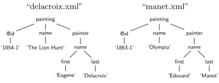
“delacroix.xml” painting @id
‘1854-1’
name ‘The Lion Hunt’
painter name first ‘Eugene’ last ‘Delacroix’ “manet.xml” painting @id ‘1863-1’ name ‘Olympia’ painter name first ‘Edouard’ last ‘Manet’
Figure 3: Sample XML documents.
For a given noden∈d, the functionkey(n) computes a string key based on whichn’s information is indexed. Lete, aandwbe three constant string tokens, andkdenote string concatenation. We definekey(n) as:
key(n) = ekn.label ifnis an XML element akn.name ifnis an XML attribute akn.name n.val wkn.val ifnis a word
Observe that we extracttwokeys from an attribute node, one to reflect the attribute name and another which reflects also its value; these help speed up specific kinds of queries, as we will see. To simplify, we omit the kwhen this does not lead to confusion.
Indexing strategies. Given a document d, an indexing
strategy I is a function that returns a set of tuples of the form (k,(a, v+)+)+. In other words,I(d) represents the set of keys k that must be added to the index store to reflect the new documentd, as well as the attributes to be stored on the respective key. Each attribute contains a nameaand a set of valuesv.
Table 2 depicts the proposed indexing strategies, which are explained in detail in the following.
5.1
Strategy
LU(Label-URI)
Index. For each node n ∈ d, strategy LU associates to
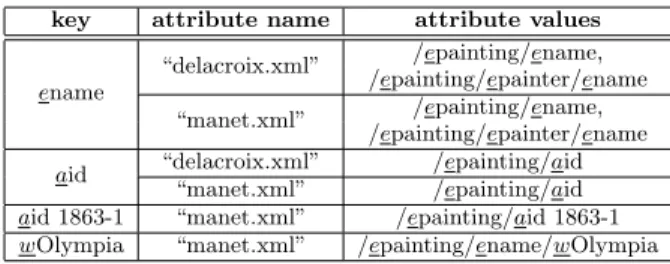
the keykey(n) the pair (URI(d), ) wheredenotes the null string. For example, applied to the documents depicted in Figure 3,LU produces among others these tuples:
key attribute name attribute values
ename “delacroix.xml” “manet.xml” aid “delacroix.xml” “manet.xml” aid 1863-1 “manet.xml” wOlympia “manet.xml”
Look-up. Given a query q expressed in the language
de-scribed in Section 4, the look-up task consists of finding, by exploiting the index, and as precisely as possible, those parts of the document warehouse that may lead to query answers. Index look-up based on theLU strategy is quite simple: all node names, attribute and element string values are ex-tracted from the query and the respective look-ups are per-formed. Then URI sets thus obtained are intersected. The query is evaluated on those documents whose URIs are part of the intersection.
5.2
Strategy
LUP(Label-URI-Path)
Index. For each node n ∈ d, LUP associates to key(n)
Name Indexing function
LU ILU(d) ={(key(n), (URI(d), ))|n∈d}
LUP ILUP(d) ={(key(n), (URI(d),{inPath1(n),inPath2(n), . . . ,inPathy(n)}))|n∈d}
LUI ILUI(d) ={(key(n), (URI(d),id1(n)kid2(n)k. . .kidz(n)))|n∈d}
2LUPI I2LUPI(d) ={[(key(n),(URI(d),{inPath1(n),inPath2(n), . . . ,inPathy(n)})),
(key(n), (URI(d),id1(n)kid2(n)k. . .kidz(n)))]|n∈d}
Table 2: Indexing strategies.
the “delacroix.xml” and “manet.xml” documents shown in Figure 3, extracted tuples include:
key attribute name attribute values
ename
“delacroix.xml” /epainting/ename, /epainting/epainter/ename “manet.xml” /epainting/ename,
/epainting/epainter/ename aid “delacroix.xml” /epainting/aid
“manet.xml” /epainting/aid aid 1863-1 “manet.xml” /epainting/aid 1863-1 wOlympia “manet.xml” /epainting/ename/wOlympia
Look-up.The look-up strategy consists of finding, for each
root-to-leaf path appearing in the query q, all documents having a data path that matches the query path. Here, a root-to-leaf query path is obtained simply by traversing the query tree and recording node keys and edge types. For instance, for the query q1 in Figure 2, the paths are: //epainting/ename and //epainting//epainter/ename. To find the URIs of all documents matching a given query path
(/|//)a1(/|//)a2. . .(/|//)aj
we look up in theLUPindex all paths associated tokey(aj), and then filter them to only those matching the path.
5.3
Strategy
LUI(Label-URI-ID)
Index. The idea of this strategy is to concatenate the
structural identifiers of a given node in a document, already
sortedby theirprecomponent, and store them into a single attribute value. We propose this implementation because structural XML joins which are used to identify the relevant documents need sorted inputs: thus, by keeping the identi-fiers ordered, we reduce the use of expensive sort operators after the look-up.
To each keykey(n), strategyLUI associates the pair (URI(d),id1(n)kid2(n)k. . .kidz(n))
such that id1(n)<id2(n)<. . .<idz(n). For instance, from the documents “delacroix.xml” and “manet.xml”, some ex-tracted tuples are:
key attribute name attribute values ename “delacroix.xml” (3,3,2)(6,8,3) “manet.xml” (3,3,2)(6,8,3) aid “delacroix.xml” (2,1,2) “manet.xml” (2,1,2) aid 1863-1 “manet.xml” (2,1,2) wOlympia “manet.xml” (4,2,3)
Look-up. Index look-up based onLUI starts by searching
the index for all the query labels. For instance, for the query q2 in Figure 2, the look-ups will beepainting,edescription, eyear and w1854. Then, the input to the Holistic Twig Join [7] must just be sorted by URI (recall that the structural identifiers for any given document are already sorted).
5.4
Strategy
2LUPI(URI-Path,
Label-URI-ID)
Index. This strategy materializes two previously
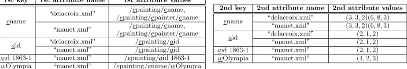
intro-duced indexes: LUPandLUI. Sample index tuples resulting from the documents in Figure 3 are shown in Figure 4.
Look-up. 2LUPI exploits, first, LUP to obtain the set
of documents containing matches for the query paths, and second,LUI to retrieve the IDs of the relevant nodes.
For instance, given the queryq2 in Figure 2, we extract the URIs of the documents matching//epainting//edescription and //epainting/eyear/w1854. The URI sets are intersected, and we obtain a relation which we denoteR1(URI). This is reminiscent of the LUP look-up. A second look-up identi-fies the structural identifiers of the XML nodes whose labels appear in the query, together with the URIs on their doc-uments. This reminds us of the LUI look-up. We denote these relations by Ra12 , R
a2 2 , . . . R
aj
2 , assuming the query node labels and values area1,a2,. . .,aj. Then:
• We compute Sai 2 = R
ai
2 <URIR1(URI) for each ai, 1≤i≤j. In other words, we useR1(URI) to reduce theR2 relations.
• We evaluate a holistic twig join overSa1 2 ,S
a2 2 ,. . .,S
aj 2 to obtain URIs of the documents with query matches. The tuples for each input of the holistic join are ob-tained by sorting the attributes by their name and then breaking down their values into individual IDs.
Figure 5 outlines this process;a1, a2, . . . , ajare the labels extracted from the query, while qp1,qp2, . . . ,qpm are the root-to-leaf paths extracted from the query.
It follows from the above explanation that2LUPI returns the same URIs asLUI. The reduction phase serves for pre-filtering, to improve performance.
5.5
Range and value-joined queries
This type of queries which are supported by our language need special evaluation strategies.
Queries with range predicates. Range look-ups in
key-value stores usually imply a full scan, which is very expen-sive. Thus, we adopt a two-step strategy. First, we perform the index look-up without taking into account the range predicate, in order to restrict the set of documents to be queried. Second, we evaluate the complete query over these documents, as usual.
Queries with value joins. Since one tree pattern only
matches one XML document, a query consisting of several tree patterns connected by a value join needs to be answered by combining tree pattern query results from different doc-uments. Indeed, this is our evaluation strategy for such queries and any given indexing strategyI: evaluate first each tree pattern individually, exploiting the index; then, apply the value joins on the tree pattern results thus obtained.
1st key 1st attribute name 1st attribute values ename “delacroix.xml” /epainting/ename, /epainting/epainter/ename “manet.xml” /epainting/ename, /epainting/epainter/ename aid “delacroix.xml” /epainting/aid
“manet.xml” /epainting/aid aid 1863-1 “manet.xml” /epainting/aid 1863-1 wOlympia “manet.xml” /epainting/ename/wOlympia
2nd key 2nd attribute name 2nd attribute values ename “delacroix.xml” (3,3,2)(6,8,3) “manet.xml” (3,3,2)(6,8,3) aid “delacroix.xml” (2,1,2) “manet.xml” (2,1,2) aid 1863-1 “manet.xml” (2,1,2) wOlympia “manet.xml” (4,2,3)
Figure 4: Sample tuples extracted by the2LUPI strategy from the documents in Figure 3.
πURI lookup(1st key=qp1) πURI lookup(1st key=qp2) . . . πURI lookup(1st key=qpm) ∩ lookup(2nd key=a1) lookup(2nd key=a2) . . . lookup(2nd key=aj) > > > > Holistic Twig Join
Figure 5: Outline of look-up using2LUPI strategy.
database1 1..ntable1 1..nitem1 1..nattribute
name 1 1 1 1..nvalue key 1 1..2
Figure 6: Structure of a DynamoDB database.
6.
CONCRETE DEPLOYMENT
As outlined before, our architecture can be deployed on top of the main existing commercial cloud platforms (see Table 1). The concrete implementation we have used for our tests relies on Amazon Web Services. In this Section, we describe the AWS components employed in the imple-mentation, and discuss their role in the whole architecture.
Amazon Simple Storage Service, or S3 in short, is a file
storage service for raw data. S3 stores the data in buckets identified by their name. Each bucket consists of a set of objects, each having an associated unique name (within the bucket), metadata (both system-defined and user-defined), an access control policy for AWS users and a version ID. We opted for storing the whole data set in one bucket because (i) in our setting we did not use e.g. different access control policies for different users, and (ii) Amazon states that the number of buckets used for a given dataset does not affect S3 storage and retrieval performance.
Amazon DynamoDB is a NoSQL database service for
storing and querying a collection of tables. Each table is a collection of items whose size can be at most 64KB. In turn, each item contains one or moreattributes; an attribute has a name, and one or several values. Each table must con-tain aprimary key, which can be either (i) a single-attribute hash key with a value of at most 2KB or (ii) a composite hash-range key that combines a 2KB hash key and a 1KB range key. Figure 6 shows the structure of a DynamoDB database. Different items within a table may have different sets of attributes.
A table can be queried through aget(T,k)operation, re-trieving all items in the tableT having a hash key valuek. If the table uses a composite hash-range key, we may use it in a call get(T,k,c) which retrieves all items in table T with hash keyk and range key satisfying the condition c. A batchGet variant permits to execute 100get operations
through a single API request. To create an item, we use theput(T,(a,v+)+)operation, which inserts the attribute(s)
(a,v+)+ into a newly created item in tableT; in this case,
(a,v+)+ must include the attribute(s) defining the primary key in T. If an item already exists with the same primary key, the new item completely replaces the existing one. A
batchPut variant inserts 25 items at a time.
Multiple tables cannot be queried by a single query. The combination of query results on different tables has to be done in the application layer.
In our system, Dynamo DB is used for storing and query-ing indexes. Previously presented indexing strategies are mapped to DynamoDB as follows. For every strategy but
2LUPI the index is stored in a single table, while for2LUPI
two different tables (one for each sub-index) are used. For any strategy, an entry is mapped into one or more items. Each item has a composite primary key, formed by a hash key and a range key. The first one corresponds to the key of the index entry, while the second one is a UUID [20]global unique identifier that can be created without a central au-thority, generated at indexing time. Attribute names and values of the entry are respectively stored into item attribute names and values.
Using UUIDs as range keys ensures that we can insert items in the index concurrently, from multiple virtual ma-chines, as items with the same hash key always contain dif-ferent range keys and thus cannot be overwritten. Also, using UUID instead of mapping each attribute name to a range key allows the system to reduce the number of items in the store for an index entry, and thus to improve perfor-mances at query time (we can recover all items for an index entry by means of a simpleget operation).
Amazon Elastic Compute Cloud, or EC2 in short,
pro-vides resizable computing capacity in the cloud. Using EC2, one can launch as many virtual computer instances as de-sired with a variety of operating systems and execute appli-cations on them.
AWS provides different types of instances, with different hardware specifications and prices, among which the users can choose: standard instances are well suited for most plications, high-memory instances for high throughput ap-plications, high-CPU instances for compute-intensive appli-cations. We have experimented with two types of standard instances, and we show in Section 8 the performance and cost differences between them.
Amazon Simple Queue Service, or SQS in short,
pro-vides reliable and scalable queues that enable asynchronous message-based communication between distributed compo-nents of an application over AWS. We rely on SQS heavily for circulating computing tasks between the various mod-ules of our architecture, that is: from the front end to the virtual instances running our indexing module for loading
and indexing the data; from the front end again to the in-stances running the query processor for answering a query, then from the query processor back to the front end to indi-cate that the query has been answered and thus the results can be fetched.
7.
APPLICATION COSTS
A relevant question in a cloud-hosted application context is, how much will this cost? Commercial cloud providers charge specific costs for the usage of their services. This sec-tion presents our model for estimating the monetary costs of uploading, indexing, hosting and querying Web data in a commercial cloud using our algorithms previously described. Section 7.1 presents the metrics used for calculating these costs, while Section 7.2 introduces the components of the cloud provider’s pricing model relevant to our application. Finally, Section 7.3 proposes the cost model for index build-ing, index storage and query answering.
7.1
Data set metrics
The following metrics capturethe impact of a given dataset, indexing strategy and queryon the charged costs.
Data-dependent metrics. Given a set of documentsD,
|D|ands(D) indicate the number of documents in D, and the total size (in GB) of all the documents inD, respectively.
Data- and index-determined metrics. For a given set
of documents D and indexing strategy I, let |op(D, I)|be the number ofput requests needed to store the index forD based on strategyI.
Let tidx(D, I) be the time needed to build and store the index for D based on strategy I. The meaningful way to measure this in a cloud is: the time elapsed between
• the moment when the first message (document load-ing request) entailed by loadload-ingDis retrieved from our application’s queue, until
• the moment when the last such message was deleted from the queue.
To compute the index size, we use:
• sr(D, I) is the raw size (in GB) of the data extracted fromDaccording toI.
• Cloud key-value stores (in our case, DynamoDB) cre-ate their own auxiliary data structures, on top of the user data they store. We denote byovh(D, I) the size (in GB) of the storage overhead incurred for the index data extracted fromDaccording toI.
Thus, the size of the data stored in an indexing service is:
s(D, I) =sr(D, I) +ovh(D, I)
Data-, index- and query-determined metrics. First,
let|r(q)|be the size (in GB) of the results for queryq. When using the indexing strategy I, for a query q and documents setD, let|op(q,D, I)|be the number ofget op-erations needed to look up documents that may contain an-swers toq, in an index forDbuilt based on the strategyI. Similarly, letDq
I be the subset of Dresulting from look-up on the index built based on strategyI for queryq.
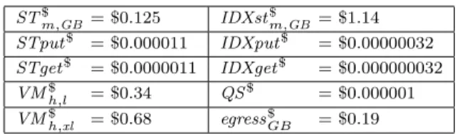
ST$ m,GB = $0.125 IDXst $ m,GB = $1.14 STput$ = $0.000011 IDXput$ = $0.00000032 STget$ = $0.0000011 IDXget$ = $0.000000032 VM$ h,l = $0.34 QS $ = $0.000001 VM$h,xl = $0.68 egress$GB = $0.19
Table 3: AWS Singapore costs as of October 2012.
Let pt(q,D) be the time needed by the query processor to answer a query q over a dataset D without using any index, and ptq(q,D, I,DqI) be the time to process q on an index built according to the strategyI(thus, on the reduced document setDq
I), respectively. We measure it as the time elapsed from the moment the message with the query was retrieved from the queue service to the moment the message was deleted from it.
7.2
Cloud services costs
We list here the costs spelled out in the the cloud service provider’s pricing policy, which impact the costs charged by the provider for our Web data management application.
File storage costs. We consider the following three
com-ponents for calculating costs associated to a file store.
• ST$
m,GB is the cost charged for storing and keeping 1 GB of data in a file store for one month.
• STput$ is the price per document storage operation request.
• STget$ is the price per document retrieval operation request.
Indexing costs. We consider the following components for
calculating the index store associated costs.
• IDX$
m,GB is the cost charged for storing and keeping 1 GB of data in the index store for one month.
• IDXput$ is the cost of aput API request that inserts a row into the index store.
• IDXget$is the cost of aget API request that retrieves a row from the index store.
Virtual instance costs. VM$
h is the price charged for running for one hour a virtual machine. This price depends on the kind of virtual machine.
Queue service costs. QS$ is the price charged for each
request to the queue service API, e.g., send message, receive message, delete message, renew lease etc.
Data transfer.The commercial cloud providers considered
in this work do not charge anything for data transferred to or within their cloud infrastructure. However, data transferred out of the cloud incurs a cost: egress$GBis the price charged for transferring 1 GB.
Concrete AWS costs vary depending on the geographic
region where AWS hosts the application. Our experiments took place in the Asia Pacific (Singapore) AWS facility, and the respective prices as of September-October 2012 are col-lected in Table 3. Note that virtual machine (instance) costs are provided for two kinds of instances, “large” (VM$h,l) and “extra-large” (VM$h,xl).
7.3
Web data management costs
We now show how to compute, based on the data-, index-and query-driven metrics (Section 7.1), together with the cloud service costs (Section 7.2), the costs incurred by our Web data storage architecture in a commercial cloud.
Indexing and storing the data.Given a set of documents
D, we calculate the cost of uploading it a file store as follows:
ud$(D) =STput$× |D|+QS$× |D|
Thus, the cost of building the index forDby means of the indexing strategyIis:
ci$(D, I) =ud$(D) +IDXput$× |op(D, I)|+STget$× |D|
+VM$
h×tidx(D, I) +QS$×2× |D|
Note that we need two queue service requests for each document: the first obtains the URI of the document that needs to be processed, while the second deletes the message from the queue when the document has been indexed.
The cost for storingDin the file store and the index struc-ture created forDaccording toI in the index store for one month is calculated as:
st$m(D, I) =ST$m,GB×s(D) +IDX $
m,GB×s(D, I)
Querying. First, we estimate the cost incurred by the
front-end for sending queryqand retrieving its results as:
rq$(q) =STget$+egress$GB× |r(q)|+QS$×3 Three queue service requests are issued: the first one sends the query, the second one retrieves the reference to the query results, and the third one deletes the message retrieved by the second request.
The cost for answering a queryqwithout using any index is calculated as follows:
cq$(q,D) =rq$(q) +STget$× |D|+STput$ +VM$h×pt(q,D) +QS$×3
Note that, again, three queue service requests are issued: the first one retrieves the message containing the query, the second one sends the message with the reference to the re-sults for the query, while the third removes the message with the query from the corresponding queue. The same holds for the formula below which calculates the cost of evaluating a queryqoverDindexed according toI:
cq$(q,D, I,DqI) =rq$(q) +IDXget$× |op(q,D, I)|
+STget$× |DIq|+STput$
+VM$h×ptq(q,D, I,DqI) +QS$×3
This finalizes our monetary cost model for Web data stores in commercial clouds, according to the architecture we de-scribed in Section 3. Some parameters of the cost model are well-known (those determined by the input data size and the provider’s cost policy), while others are query- and strategy-dependent (e.g., how may documents match a query etc.) In Section 8 we measure actual charged costs, where the query-and strategy-dependent parameters are instantiated to con-crete operations. These measures allow to highlight the cost savings brought by our indexing.
Indexing strategy Average ex-traction time (hh:mm) Average up-loading time (hh:mm) Total time (hh:mm) LU 0:24 1:33 2:11 LUP 0:32 3:47 4:25 LUI 0:41 2:31 3:22 2LUPI 1:13 6:30 7:46
Table 4: Indexing times using 8 large (L) instances.
8.
EXPERIMENTAL RESULTS
This section describes the experimental environment and results obtained. Section 8.1 describes the experimental setup, Section 8.2 reports our performance results, and fi-nally, Section 8.3 presents our cost study.
8.1
Experimental setup
Our experiments ran on AWS servers from the Asia Pa-cific region in September-October 2012. We used the (cen-tralized) Java-based XML query processor developed within our ViP2P project [16], implementing an extension of the algorithm of [9] to our larger subset of XQuery. On this dialect, our experiments have shown that ViP2P’s perfor-mance is close to (or better than) Saxon-B v9.12.
We use two types of EC2 instances for running the index-ing module and query processor:
• Large (l), with 7.5 GB of RAM memory and 2 virtual
cores with 2 EC2 Compute Units each.
• Extra large (xl), with 15 GB of RAM memory and
4 virtual cores with 2 EC2 Compute Units each.
An EC2 Compute Unit is equivalent to the CPU capacity of a 1.0-1.2 GHz 2007 Xeon processor.
To test index selectivity, we needed an XML corpus with some heterogeneity. We generated XMark [24] documents (20000 documents in all, adding up to 40 GB), using the
split option provided by the data generator3. We modi-fied a fraction of the documents to alter theirpathstructure (while preserving their labels), and modified another frac-tion to make them “more” heterogeneous than the original documents, by rendering more elements optional children of their parents, whereas they were compulsory in XMark.
8.2
Performance study
XML indexing. To test the performance of index creation,
the documents were initially stored in S3, from which they were gathered in batches by multiple l instances running the indexing module. We batched the documents in order to minimize the number of calls needed to load the index into DynamoDB. Moreover, we usedlinstances because in our configuration, DynamoDB was the bottleneck while in-dexing. Thus, using more powerful xlinstances could not have increased the throughput.
Table 4 shows the time spent extracting index entries on 8
lEC2 instances and uploading the index to DynamoDB us-ing each proposed strategy. We show the average time spent by each EC2 machine to extract the entries, the average time spent by DynamoDB to load the index data, and the total observed time (elapsed between the beginning and the end of the overall indexing process). As expected, the more and
2http://saxon.sourceforge.net/
3
0! 5000! 10000! 15000! 20000! 25000! 30000! 0! 10! 20! 30! 40! In d e x in g ti m e (s ) ! Documents size (GB)!
LU! LUP! LUI! 2LUPI!
Figure 7: Indexing in 8 large (L) EC2 instances.
0! 15! 30! 45! 60! 75! 90! 105! 120! 135! 0! 20! 40! 60! 80! 100! 120!
LU! LUP! LUI! 2LUPI!
C o s t ($ /m o n th ) ! Si ze (G B ) !
DynamoDB overhead data! Index content! XML data size! 0! 15! 30! 45! 0! 10! 20! 30! 40!
LU! LUP! LUI! 2LUPI!
C o s t ($ /m o n th ) ! Si ze (G B ) !
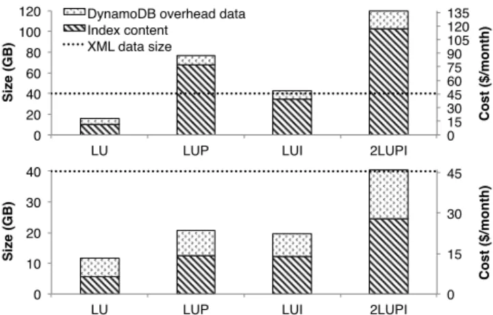
Figure 8: Index size and storage costs per month with full-text indexing (top) and without (bottom).
Query # Doc. IDs from index # Docs. Results LU LUP LUI 2LUPI w. results size (KB)
q1 3 2 1 1 1 0.04 q2 523 349 349 349 349 94000.00 q3 144 66 33 33 33 52400.00 q4 1089 1089 775 775 775 519.20 q5 1115 740 370 370 370 7500.00 q6 285 283 283 283 283 278.20 q7 285 283 142 142 142 96.20 q8 1400 1025 882 882 507 13800.00 q9 1115 740 740 740 740 338800.00 q10 1400 1025 512 512 116 9.10
Table 5: Query processing details (20000
docu-ments).
the larger the entries a strategy produces, the longer index-ing takes. Next, Figure 7 shows that indexindex-ing time scales well, linearly in the size of the data for each strategy.
A different perspective on the indexing is given in Figure 8 which shows the size of the index entries, compared with the original XML size. In addition to the full-text indexes size, the figure includes the size for each strategy if keywords are not stored. As expected, the index for the latter strategies is quite smaller than the full-text variant. LUP and2LUPI
are the larger indexes, and in particular, if we index the keywords, the index is quite larger than the data. TheLUI
index is smaller than the LUP one, because IDs are more compact than paths; moreover, we exploit the fact that Dy-namoDB allows storing arbitrary binary objects, to store compressed (encoded) sets of IDs in a single DynamoDB value. Finally, the DynamoDB space overhead (Section 7) is noticeable, especially if keywords are not indexed, but in both variants grows slower than the index size.
XML query processing.We now study the query
process-ing performance, usprocess-ing 10 queries from the XMark bench-mark; they can be found in the Appendix. The queries have
an average of ten nodes each; the last three queries feature value joins.
Table 5 shows, for each query and indexing strategy, the number of documents retrieved by index look-up, the num-ber of documents which actually contain query results, and the result size for each query. (These are obviously inde-pendent of the platform, and we provide them only to help interpret our next results.) Table 5 shows that LUI and
2LUPI are exact for queries q1-q7, which are tree pattern queries (the look-up in the index returns no false positive in these cases). The imprecision ofLUandLUP varies across the queries, but it may reach 200% (twice as many false positives, as there are documents with results), even for tree pattern queries likeq5. For the last three queries, featuring value joins, even LUIand LUPImay bring false positives. For these queries, Table 5 sums the numbers of document IDs retrieved for each tree pattern.
The response times (perceived by the user) for each query, using each indexing strategy, and also without any index, is shown in Figure 9a; note the logarithmic y axis. We have evaluated the workload usingland then, separately,xlEC2 instances. We see that all indexes considerably speed up each query, by one or two orders of magnitude in most cases. Figure 9a also demonstrates that our strategies are able to take advantage of more powerful EC2 instances, that is, for every query, thexlrunning times are shorter than the times using an linstance. The strategy with the shortest evalu-ation time is LUP, which strikes a good balance between precision and efficiency; most of the time, LUis next, fol-lowed by LUI and 2LUPI (recall again that the y axis is log-scale). The difference between the slowest and fastest strategy is a factor of 4 at most whereas the difference be-tween the fastest index and no index is of 20 at least.
The charts in Figures 9b and 9c provide more insight. They split query processing time into: the time to consult the index (DynamoDB get), the time to run the physical plan identifying the relevant document URIs out of the data retrieved from the index, and the time to fetch the doc-uments from S3 into EC2 and evaluate the queries there.
Importantly, since we make use of the multi-core capabilities of EC2 virtual machines, the times individually reported in Figures 9b and 9c were in fact measured in parallel. In other words, the overall response time observed and reported in Figure 9a is systematically less than the sum of the detailed times reported in Figures 9b and 9c.
We see that low-granularity indexing strategies (LU and
LUP) have systematically shorter index look-up and index post-processing times than the fine-granularity ones (LUI
and2LUPI). The times to transfer the relevant documents to EC2 and evaluate queries there, is proportional to the num-ber of documents retrieved from the index look-ups (these numbers are provided in Table 5). For a given query, the document transfer + query evaluation time differs between the strategies by the factor of up to 3, corresponding to the number of documents retrieved.
Impact of parallelism. Figure 10 shows how the query
response time varies when running multiple EC2 query pro-cessing instances. To this purpose, we sent to the front-end all our workload queries, successively, 16 times:q1, q2, . . . , q10, q1, q2, . . .etc. We report the running times on a single EC2 instance (no parallelism) versus running times on eight EC2 instances in parallel. We can see that more instances signifi-cantly reduce the running time, more so forlinstances than
0.1! 1! 10! 100! 1000! 10000! L! XL! L! XL! L! XL! L! XL! L! XL! L! XL! L! XL! L! XL! L! XL! L! XL! q1! q2! q3! q4! q5! q6! q7! q8! q9! q10! R e s p o n s e T im e (s ) !
No Index! LU! LUP! LUI! 2LUPI!
(a) Response time using large (l) and extra large (xl) EC2 instances on the 40 GB database
0.1! 1! 10! 100! 1000! LU ! L U P ! LUI ! 2 L U PI ! LU ! L U P ! LUI ! 2 L U PI ! LU ! L U P ! LUI ! 2 L U PI ! LU ! L U P ! LUI ! 2 L U PI ! LU ! L U P ! LUI ! 2 L U PI ! LU ! L U P ! LUI ! 2 L U PI ! LU ! L U P ! LUI ! 2 L U PI ! LU ! L U P ! LUI ! 2 L U PI ! LU ! L U P ! LUI ! 2 L U PI ! LU ! L U P ! LUI ! 2 L U PI ! q1! q2! q3! q4! q5! q6! q7! q8! q9! q10! T im e (s ) !
Lookup - DynamoDB Get! Lookup - Plan execution! S3 documents transfer and results extraction!
(b) Detail large (l) EC2 instance on the 40 GB database
0.1! 1! 10! 100! 1000! LU ! L U P ! LUI ! 2 L U PI ! LU ! L U P ! LUI ! 2 L U PI ! LU ! L U P ! LUI ! 2 L U PI ! LU ! L U P ! LUI ! 2 L U PI ! LU ! L U P ! LUI ! 2 L U PI ! LU ! L U P ! LUI ! 2 L U PI ! LU ! L U P ! LUI ! 2 L U PI ! LU ! L U P ! LUI ! 2 L U PI ! LU ! L U P ! LUI ! 2 L U PI ! LU ! L U P ! LUI ! 2 L U PI ! q1! q2! q3! q4! q5! q6! q7! q8! q9! q10! T im e (s ) !
Lookup - DynamoDB Get! Lookup - Plan execution! S3 documents transfer and results extraction!
(c) Detail extra large (xl) EC2 instance on the 40 GB database
Figure 9: Response time (top) and details (middle and bottom) for each query and indexing strategy.
0! 6000! 12000! 18000! 24000! 30000! 36000!
LU! LUP! LUI! 2LUPI! LU! LUP! LUI! 2LUPI!
L! XL! R e s p o n s e T im e (s ) ! 1 instance! 8 instances!
Figure 10: Impact of using multiple EC2 instances.
Indexing DynamoDB EC2 S3 + SQS Total
strategy LU $21.15 $5.47 $0.02 $26.64 LUP $44.78 $11.95 $56.75 LUI $33.47 $8.95 $42.44 2LUPI $78.25 $21.17 $99.44
Table 6: Indexing costs for 40 GB using L instances.
forxl ones: this is because many strong instances sending indexing requests in parallel come close to saturating Dy-namoDB’s capacity of absorbing them.
8.3
Amazon charged costs
We now study the costs charged by AWS for indexing the data, and for answering queries. We also consider the amor-tization of the index, i.e., when query cost savings brought by the index balance the cost of the index itself.
Indexing cost. Table 6 shows the monetary costs for
in-dexing data according to each strategy. These costs are bro-ken down across the specific AWS services. The most costly index to build is2LUPI, while the cheapest isLU. The com-bined price for S3 and SQS is constant across strategies, and
is negligible compared to EC2 costs. In turn, the EC2 cost is dominated by the DynamoDB cost in all strategies.
Finally, Figure 8 shows the storage cost per month of each index, which is proportional to its size in DynamoDB.
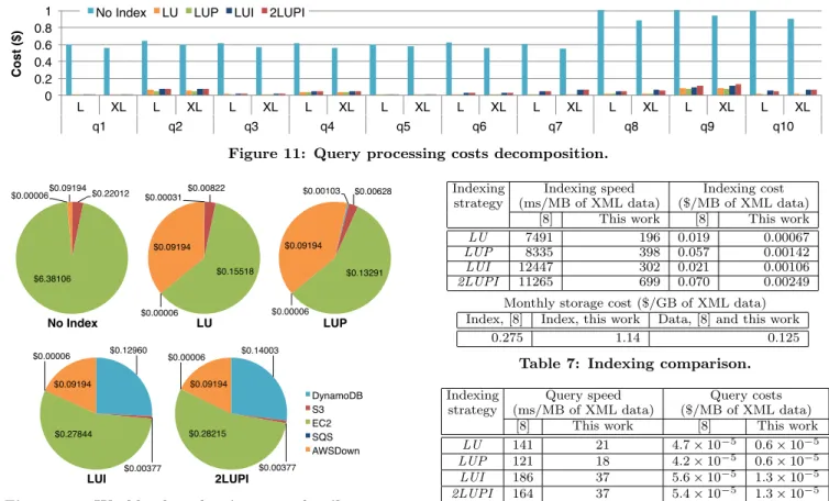
Query processing cost. Figure 11 shows the cost of
an-swering each query when using no index, and when using the different indexing strategies. Note that using indexes, the cost is practically independent of the machine type. This is because (i) the hourly cost for an xlmachine is double than that of a l machine; but at the same time (ii) the four cores of anxlmachine allow processing queries simul-taneously on twice as many documents as the two cores of
l machines, so that the cost differences pretty much
can-cel each other (whereas thetimedifferences are noticeable). Figure 11 also shows thatindexing significantly reduces mon-etary costscompared to the case where no index is used; the savings vary between 92% and 97%.
To better understand the monetary costs shown in Fig-ure 11, we provide the details of evaluating the query work-load on an xl instance in Figure 12, again decomposed across the services we use, to which we addAWSDown, the price charged by Amazon for transferring query results out of AWS.AWSDowncost is the same for all strategies, since the same results are obtained. S3 cost is proportional to the selectivity of the index strategy (recall Table 5). DynamoDB costs reflect the amount of data extracted for each strategy from the index, and finally, EC2 cost is proportional to the time necessary to answer the workload using each strategy, which means that the shorter it takes to answer a query, the
0! 0.2! 0.4! 0.6! 0.8! 1! L! XL! L! XL! L! XL! L! XL! L! XL! L! XL! L! XL! L! XL! L! XL! L! XL! q1! q2! q3! q4! q5! q6! q7! q8! q9! q10! C o s t ($ ) !
No Index! LU! LUP! LUI! 2LUPI!
Figure 11: Query processing costs decomposition. $0.22012! $6.38106! $0.00006!$0.09194! No Index! DynamoDB! S3! EC2! SQS! AWSDown! $0.00031!$0.00822! $0.15518! $0.00006! $0.09194! LU! DynamoDB! S3! EC2! SQS! AWSDown! $0.00103! $0.00628! $0.13291! $0.00006! $0.09194! LUP! DynamoDB! S3! EC2! SQS! AWSDown! $0.12960! $0.00377! $0.27844! $0.00006! $0.09194! LUI! DynamoDB! S3! EC2! SQS! AWSDown! $0.14003! $0.00377! $0.28215! $0.00006! $0.09194! 2LUPI! DynamoDB! S3! EC2! SQS! AWSDown!
Figure 12: Workload evaluation cost details on an extra large (XL) instance.
-100-75!! -50! -25! 0! 25! 50! 75! 100! 125! 0! 2! 4! 6! 8! 10! 12! 14! 16! 18! 20! # ru n s x b e n e fi t( I , W ) - b u il d in g C o s t( I ) ! # runs!
LU! LUP! LUI! 2LUPI!
Figure 13: Index cost amortization for a single extra large (XL) EC2 instance.
lower it will be its cost. For every strategy, the cost of using EC2 clearly dominates, which is expected and desired, since this is the time actually spent processing the query.
Amortization of the index costs. We now study how
indexing pays off when evaluating queries. For an indexing strategyI and workloadW, we termbenefitofIforW the difference between the monetary cost to answerW using no index, and the cost to answerW based on the index built according to I. At each run of W, we “save” this bene-fit, whereas we had to pay a certain cost to buildI. (The index costs and benefits also depend on the data set, and increase with its size.) Figure 13 shows when the cumulated benefit (over several runs of the workload on alinstance) overweighs the index building cost (similarly, on a singlel
instance, recall Table 6). Figure 13 shows that any of our strategies allows recovering the index creation costs quite fast, i.e. just running the workload 4 times forLU, 8 times forLUPandLUI, and16times for2LUPIrespectively. (The cost is recovered when the curves cross theY = 0 axis.)
Indexing Indexing speed Indexing cost
strategy (ms/MB of XML data) ($/MB of XML data)
[8] This work [8] This work
LU 7491 196 0.019 0.00067
LUP 8335 398 0.057 0.00142
LUI 12447 302 0.021 0.00106
2LUPI 11265 699 0.070 0.00249
Monthly storage cost ($/GB of XML data) Index, [8] Index, this work Data, [8] and this work
0.275 1.14 0.125
Table 7: Indexing comparison.
Indexing Query speed Query costs
strategy (ms/MB of XML data) ($/MB of XML data)
[8] This work [8] This work
LU 141 21 4.7×10⁻⁵ 0.6×10⁻⁵
LUP 121 18 4.2×10⁻⁵ 0.6×10⁻⁵
LUI 186 37 5.6×10⁻⁵ 1.3×10⁻⁵
2LUPI 164 37 5.4×10⁻⁵ 1.3×10⁻⁵
Table 8: Query processing comparison.
8.4
Comparison with previous works
The closest related works are [6, 19] and our previous work [8], which build database services on top of a com-mercial cloud, and in particular AWS.
The focus in [6] was on implementing transactions in the cloud with various consistency models; they present exper-iments on the TPC-W relational benchmark, using 10.000 products (thus, a database of 315 MB of data, about 125 times smaller than ours). The setting thus is quite differ-ent, but a rough comparison can still be done.
At that time, Amazon did not provide a key-value store, therefore the authors built B+ trees indexes within S3. Each
transactionin [6] retrieves one customer record, searches for six products, and orders three of them. These are all selec-tive (point) queries (and updates), thus, they only compare withq1among our queries, the only one which can be assim-ilated to a point query (very selective path matched in few documents, recall Table 5). For atransaction, they report running times between 2.8 and 11.3 seconds, while individ-ual queries/updates are said to last less than a second. Our q1, running in 0.5 seconds (using one instance) on our 40 GB database of data, is thus quite competitive. Moreover, [6] re-ports transaction costs between $1.5×10⁻⁴and $2.9×10⁻³, very close to our $1.2×10⁻⁴ cost ofq1 usingLUP.
Next, we compare with our previous work [8], evaluated on only 1 GB of XML data. From a performance perspec-tive, the main difference is that [8] stores the index within AWS’ previous key-value store, namely SimpleDB. Table 7 compares this work with [8] from the perspective of index-ing, and Table 8 from that of querying; for a fair comparison, we report measuresper MB (or GB)of data.
index-ing by one to two orders of magnitude, all the while index-ing costs are reduced by two to three orders of magnitude;
querying is faster (and query costs lower) by a factor of five
(roughly) wrt [8]. The reason is that DynamoDB allows stor-ing arbitrary binary objects as values, a feature we exploited in order to efficiently encode our index data. Moreover, Dy-namoDB has a shorter response time and can handle more concurrent requests than SimpleDB.
The authors of [6] subsequently also ported their index to SimpleDB [19]. Still on TPC-W transactions on a 10.000 items database, processing with a SimpleDB index was mod-erately faster (by a factor of less than 2) than by using their previous S3-based one. As we have seen above, DynamoDB significantly outperforms SimpleDB when indexing.
8.5
Experiments conclusion
Our experiments demonstrate the feasibility and interest of our architecture based on a commercial cloud, using a distributed file system to store XML data, a key-value store to store the index, and the cloud’s processing engines to in-dex and process queries. All our inin-dexing strategies have been shown to reduce query response time and monetary cost, by 2 orders of magnitude in our experiments; more-over, our architecture is capable of scaling up as more in-stances are added. The monetary costs of query processing are shown to be quite competitive, compared with previous similar works [6, 8], and we have shown that the overhead of building and maintaining the index is modest, and quickly offset by the cost savings due to the ability to narrow the query to only a subset of the documents. In our tests, the
LUPindexing strategy allowed for the most efficient query processing, at the expense of an index size somehow larger than the data. Further compression of the paths in theLUP
index could probably make it even more competitive. In our experiments, query execution based on the LU and LUP strategies is always faster than using the LUI and 2LUPI strategies. We believe that cases for which LUI and 2LUPI strategies behave better are those in which query tree patterns are multi-branched, highly selective and evalu-ated over a document set where most of the documentsonly
match linear paths of the query. Such cases can be stati-cally detected by using data summaries and some statistical information. We postpone this study to future work.
9.
CONCLUSION
We have presented an architecture for building scalable XML warehouses by means of commercial cloud resources, which can exploit parallelism to speed up index building and query processing. We have investigated and compared through experiments several indexing strategies and shown that they achieve query processing speed-up and monetary costs reductions of several orders of magnitude within AWS. Our future works include the development of a platform and index advisor tool, which based on the expected dataset and workload, estimates an application’s performance and cost and picks the best indexing strategy to use.
Acknowledgments
This work has been partially funded by the KIC EIT ICT Labs activities 11803, 11880 and RCLD 12115, as well as an AWS in Education research grant.
10.
REFERENCES
[1] S. Abiteboul, S. Cluet, G. Ferran, and M.-C. Rousset. The Xyleme project.Computer Networks, 39(3), 2002. [2] S. Abiteboul, I. Manolescu, N. Polyzotis, N. Preda, and
C. Sun. XML processing in DHT networks. InICDE, 2008. [3] S. Al-Khalifa, H. V. Jagadish, J. M. Patel, Y. Wu,
N. Koudas, and D. Srivastava. Structural Joins: A Primitive for Efficient XML Query Pattern Matching. In ICDE, 2002.
[4] A. Aranda-And´ujar, F. Bugiotti, J. Camacho-Rodr´ıguez, D. Colazzo, F. Goasdou´e, Z. Kaoudi, and I. Manolescu. AMADA: Web Data Repositories in the Amazon Cloud (demo). InCIKM, 2012.
[5] P. A. Bernstein, I. Cseri, N. Dani, N. Ellis, A. Kalhan, G. Kakivaya, D. B. Lomet, R. Manne, L. Novik, and T. Talius. Adapting Microsoft SQL server for cloud computing. InICDE, 2011.
[6] M. Brantner, D. Florescu, D. A. Graf, D. Kossmann, and T. Kraska. Building a database on S3. InSIGMOD, 2008. [7] N. Bruno, N. Koudas, and D. Srivastava. Holistic twig
joins: optimal XML pattern matching. InSIGMOD, 2002. [8] J. Camacho-Rodr´ıguez, D. Colazzo, and I. Manolescu.
Building Large XML Stores in the Amazon Cloud. InDMC Workshop (collocated with ICDE), 2012.
[9] Y. Chen, S. B. Davidson, and Y. Zheng. An Efficient XPath Query Processor for XML Streams. InICDE, 2006. [10] H. Choi, K.-H. Lee, S.-H. Kim, Y.-J. Lee, and B. Moon.
HadoopXML: A Suite for Parallel Processing of Massive XML Data with Multiple Twig Pattern Queries (demo). In CIKM, 2012.
[11] L. Fegaras, C. Li, U. Gupta, and J. Philip. XML Query Optimization in Map-Reduce. InWebDB, 2011.
[12] L. Galanis, Y. Wang, S. Jeffery, and D. DeWitt. Locating data sources in large distributed systems. InVLDB, 2003. [13] R. Goldman and J. Widom. Dataguides: Enabling query
formulation and optimization in semistructured databases. InVLDB, 1997.
[14] V. Kantere, D. Dash, G. Fran¸cois, S. Kyriakopoulou, and A. Ailamaki. Optimal service pricing for a cloud cache. IEEE Trans. Knowl. Data Eng., 23(9), 2011.
[15] V. Kantere, D. Dash, G. Gratsias, and A. Ailamaki. Predicting cost amortization for query services. In SIGMOD, 2011.
[16] K. Karanasos, A. Katsifodimos, I. Manolescu, and S. Zoupanos. The ViP2P Platform: XML Views in P2P. In ICWE, 2012.
[17] R. Kaushik, P. Bohannon, J. F. Naughton, and H. F. Korth. Covering indexes for branching path queries. In SIGMOD, 2002.
[18] G. Koloniari and E. Pitoura. Peer-to-peer management of XML data: issues and research challenges.SIGMOD Record, 34(2), 2005.
[19] D. Kossmann, T. Kraska, and S. Loesing. An evaluation of alternative architectures for transaction processing in the cloud. InSIGMOD, 2010.
[20] P. Leach, M. Mealling, and R. Salz. A Universally Unique IDentifier (UUID) URN Namespace. IETF RFC 4122, July 2005.
[21] I. Manolescu, K. Karanasos, V. Vassalos, and S. Zoupanos. Efficient XQuery rewriting using multiple views. InICDE, 2011.
[22] T. Milo and D. Suciu. Index structures for path expressions. InICDT, 1999.
[23] J. Schad, J. Dittrich, and J.-A. Quian´e-Ruiz. Runtime Measurements in the Cloud: Observing, Analyzing, and Reducing Variance.PVLDB, 3(1), 2010.
[24] A. Schmidt, F. Waas, M. L. Kersten, M. J. Carey, I. Manolescu, and R. Busse. XMark: A benchmark for XML data management. InVLDB, 2002.
APPENDIX
We provide here additional details on our experiments.
A.
QUERY WORKLOAD DETAILS
Figure 14 depicts the workload used in the experimental section; it consists of 10 queries with an average of 10 nodes each. The queries are taken from the XMark benchmark. Three workload queries contained value joins, the other each correspond to a tree pattern. Furthermore, queryq1 is very selective (point query); queryq4uses a full-text search pred-icate.
B.
EXPERIMENTAL RESULTS WITHOUT
KEYWORDS
Indexing strategy Average ex-traction time (hh:mm) Average up-loading time (hh:mm) Total time (hh:mm) LU 0:05 1:32 1:44 LUP 0:06 2:08 2:20 LUI 0:09 2:13 2:28 2LUPI 0:15 4:20 4:46Table 9: Indexing times details using 8 large (L) EC2 instances (40 GB database).
Query # Doc. IDs from index # Docs. Results LU LUP LUI 2LUPI w. results size (KB)
q1 3 2 1 1 1 0.04 q2 523 349 349 349 349 94000.00 q3 144 66 33 33 33 52400.00 q4 1089 1089 775 775 775 519.20 q5 1115 740 370 370 370 7500.00 q6 285 283 283 283 283 278.20 q7 285 283 142 142 142 96.20 q8 1400 1025 882 882 507 13800.00 q9 1115 740 740 740 740 338800.00 q10 1400 1025 512 512 116 9.10
Table 10: Queries response detail without using
key-words (20.000documents).
Indexing DynamoDB EC2 S3 + SQS Total
strategy LU 19.29 4.56 0.02 23.86 LUP 26.32 6.26 32.60 LUI 25.38 6.61 32.00 2LUPI 51.70 12.93 64.64
Table 11: Cost detail [$] for indexing the 40 GB database using large (L) EC2 instance(s).
q1
site
people
person
@id=person0 nameval q2 site open auctions open auction bidder increaseval q3 site regions australia item
nameval descriptioncont q4
site
item
description
textcontains(gold)
nameval q5
site
people
person
homepage nameval q6 site closed auctions closed auction annotation description parlist listitem parlist listitem text emph keywordval q7 site closed auctions closed auction annotation description parlist listitem parlist listitem text emph keywordval seller @personval q8 site people person
@id nameval
site closed auctions closed auction buyer @person itemref @itemval q9 site people person profile
genderval ageval educationval @incomeval interest
@category site people person profileval interest @category q10 site closed auctions closed auction
quantity=2 type=Regular buyerval
@person
site
people
person
@idval name gender=f emale business=Y es country=U nited States
Figure 14: Query workload used in the experimental section.
0.001! 0.01! 0.1! 1! 10! 100! 1000!
KW! NoKW!KW!NoKW!KW!NoKW!KW! NoKW!KW!NoKW! KW! NoKW!KW!NoKW! KW! NoKW!KW!NoKW! KW!NoKW!
q1! q2! q3! q4! q5! q6! q7! q8! q9! q10! R e s p o n s e T im e (s ) !
LU! LUP! LUI! 2LUPI!
Figure 15: Response time using large (L) EC2 instances on the 40 GB database with and without using keywords (KW and NoKW, respectively).