Boundary Condition Study for the Juncture Flow Experiment in the NASA Langley 14x22-Foot Subsonic Wind Tunnel

Boundary Condition Study for the Juncture Flow Experiment

in the NASA Langley 14x22-Foot Subsonic Wind Tunnel

C. L. Rumsey

, J.-R. Carlson

, J. A. Hannon

, L. N. Jenkins

, S. M. Bartram

NASA Langley Research Center, Hampton, VA 23681

T. H. Pulliam

NASA Ames Research Center, Moffett Field, CA 94035

H. C. Lee

Science and Technology Corporation, Moffett Field, CA 94035

Because future wind tunnel tests associated with the NASA Juncture Flow project are being designed for the purpose of CFD validation, considerable effort is going into the characterization of the wind tunnel boundary conditions, particularly at inflow. This is important not only because wind tunnel flowfield nonuniformities can play a role in integrated testing uncertainties, but also because the better the boundary conditions are known, the better CFD can accurately represent the experiment. This paper describes recent investigative wind tunnel tests involving two methods to measure and characterize the oncoming flow in the NASA Langley 14- by 22-Foot Subsonic Tunnel. The features of each method, as well as some of their pros and cons, are highlighted. Boundary conditions and modeling tactics currently used by CFD for empty-tunnel simulations are also described, and some results using three different CFD codes are shown. Preliminary CFD parametric studies associated with the Juncture Flow model are summarized, to determine sensitivities of the flow near the wing-body juncture region of the model to a variety of modeling decisions.

I.

Introduction

The NASA Juncture Flow (JF) experiment1, 2 _{has been in the planning stages for some time. The test, planned} for late 2017 and early 2018 in the NASA Langley 14- by 22-Foot Subsonic Tunnel (14x22), is designed to measure CFD-validation-quality data for the onset and progression of a trailing edge separation near the wing-body juncture of an aircraft-like configuration. These particular flow features are considered to be difficult for state-of-the-art CFD methods to reliably predict.3 _{The experiment will provide a significant amount of detailed information to help enable} improvement in the methods.

In work leading up to the final experiments, several risk-reduction experiments were conducted in conjunction with CFD studies, to down-select to appropriate configuration(s). The JF team originally desired to find a wing-body configuration that could achieve fully-attached flow, incipient corner separation, and separated corner flow by varying either the freestream Mach number or the model angle of attack. Unfortunately, this was not possible, so the final down-select included two different sets of wings.2 The primary configuration is the DLR-F6 wing,3which achieves a corner flow separation at all angles of attack (AoA orα) in the range−10< α <10deg. (The separation size grows with angle of attack.) The secondary configuration is a symmetric wing with an NACA 0015 shape at the root. In the risk-reduction tests, the 0015-based wing achieved fully-attached flow up to aboutα= 5deg., and only a very small corner separation at higher angles of attack.

In the 2017-2018 experimental campaign, laser Doppler velocimetry (LDV) and particle image velocimetry (PIV) will be used to document the flow field upstream and within the corner separation region. The LDV system will be

∗_{Research Scientist, Computational AeroSciences Branch, Mail Stop 128, Fellow AIAA.} †_{Research Scientist, Computational AeroSciences Branch, Mail Stop 128, Senior Member AIAA.} ‡_{Research Scientist, Flow Physics and Control Branch, Mail Stop 170.}

§_{Research Scientist, Flow Physics and Control Branch, Mail Stop 170.}

¶_{Engineering Technician, Advanced Measurements and Data Systems Branch, Mail Stop 493.} k_{Research Scientist, Computational Aerosciences Branch, Mail Stop 258-2, Associate Fellow AIAA.} ∗∗_{Research Scientist, Computational Aerosciences Branch, Mail Stop 258-2, Member AIAA.}

carried inside the model’s fuselage, and its lasers will pass through windows installed on the side of the model near several regions of interest. These regions include the wing trailing edge area (where the separation occurs), as well as the wing leading edge area and an area well upstream on the fuselage nose. The latter two areas will help to establish oncoming boundary conditions for use in CFD.

For this experiment, the JF team would like to assess, and document where possible, the larger-field tunnel bound-ary conditions (particularly the inflow near the start of the test section). These boundbound-ary conditions are considered important inputs for CFD validation; also, flowfield nonuniformities may influence integrated testing uncertainties.4 Making these types of measurements is a challenging task, so CFD will likely eventually end up playing a part in this assessment, as described in this paper. The importance of this type of wind tunnel documentation has been cited in the literature.5, 6_{To initiate an assessment for the JF project (and to contribute to the larger effort to better understand wind} tunnel boundary conditions in general), several wind tunnel tests were conducted in the 14x22 during 2016. One of these tests involved the Boeing Quantitative Wake-Survey System (QWSS)7, 8 _{MK-17 device. This device (described} in Section IIB) has a movable 5-hole probe designed primarily for performing field measurements in wakes. Here, we assess its capability to measure nonuniformity levels in the wind tunnel free stream. The pros and cons of using PIV for measuring the free stream were also explored, as described in Section IIC. Section III covers the CFD simulations performed for this work.

The main purposes of this paper are: (1) document the recent QWSS and PIV tests, (2) explore boundary conditions for running empty tunnel simulations in CFD, and (3) perform parametric CFD studies to show the influence of various global modeling “decisions” on the JF model region of interest. This latter type of study, taken further, could perhaps help to quantify uncertainty levels caused by wind tunnel nonuniformities that are difficult to measure. This paper touches on several areas that are believed to impact the fidelity with which CFD is able to mimic a wind tunnel experiment. Because of the wide range covered, the paper should be considered as more of an overview, rather than an in-depth study on a particular topic.

II.

Preparatory Wind Tunnel Experiments

In this section, we describe recent wind tunnel experiments in the 14x22, which is a closed-loop tunnel. A diagram of the high-speed leg of this tunnel is shown in Fig. 1. These tests were conducted primarily for the purpose of evaluating the efficacy of the QWSS and PIV for determining inflow boundary conditions in this wind tunnel. However, they also included some additional measurements of side- and top-wall boundary layers, wall pressures in the test section, and bottom wall pressures in the diffuser. Among these, we only briefly show the latter in Subsection A. For the QWSS and PIV, covered in Subsections B and C, respectively, we try to answer the following questions. How useful and how accurate are these techniques? If useful, then can they be used once (in an empty tunnel) to determine the inflow BCs, or must they be remeasured every time a different model is introduced?

A. Diffuser Pressures

Generally speaking, measurements of boundary conditions (upstream, downstream, walls) are all useful additions for any tunnel experiment whose purpose is CFD validation. The more data collected in the tunnel toward helping to establish the flow conditions, the better. An example is shown in Fig. 2, for pressures collected along the bottom wall of the diffuser during the QWSS testing. CFD results from an empty tunnel run (to be discussed later) are included in the figure for reference, and the agreement between CFD and experiment is very close. However, note that these are not direct one-to-one comparisons, since the experiment included the QWSS device and the CFD did not. The main point here is that with tunnel diffuser pressure measured, CFD could either (1) further validate its method for achieving the correct tunnel flow conditions, or (2) make use of the tunnel back pressure data to set its boundary conditions. B. Quantitative Wake Survey System (QWSS)

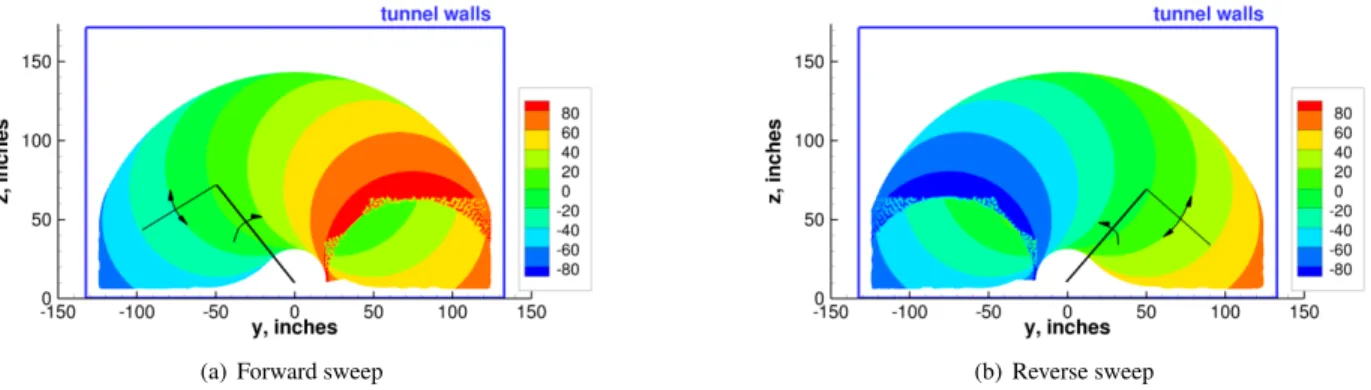
Boeing’s QWSS MK-17 device (Fig. 3) holds a 5-hole flow angularity probe mounted on the end of a traversing mechanism that continuously sweeps the probe over a large area, allowing a region of the flow field to be mapped to within approximately one-quarter inch resolution. There are two arms, each of which can rotate about its respective motor. A photograph of the QWSS in the 14x22 is shown in Fig. 3(b). Because of its size and large range of motion, the QWSS can cover a significant fraction of the 14x22’s width and height. Figure 4 shows contour examples of the large sweep area covered by QWSS with its larger bottom arm sweeping from left-to-right (“forward sweep”), and right-to-left (“reverse sweep”). The peak height reached in the center of the tunnel was approximately142 inches above the tunnel floor. Note that a large region in the center area can be measured with the arms in two different

Figure 1. As-built high-speed leg of the 14x22.

orientations, but the lowest regions to the bottom left and bottom right can only be obtained with the arms in one particular orientation. The arm positions for the two sweeping motion directions will prove important, as described below.

The 5-hole probe was calibrated to attain static and total pressures, as well as local flow angles. Here we focus on the local flow angles only; the pressures are not discussed in this paper. Theαprb andβprbare the local pitch and

yaw angles of the flow as measured by the probe in the probe coordinate system. These angles are determined based on∆pfrom the four static pressures on the sides of the conical probe section, taking into account any motion of the probe as it sweeps. Then, from the angular position of both traversing arms at any point in its sweeping path, the angle

ΘP of the probe relative to the tunnel is known. From this information, theαtunn andβtunn (local pitch and yaw

angles of the flow in the tunnel coordinate system) are derived from geometric relations. Figure 5 is an example of the angularity probe in the same physical location but the traversing arms in two different orientations, showing how the position of the arms causes the probe to be rotated differently with respect to tunnel coordinates. Note that the QWSS historically has only been used for wake surveys with primary interest in mean flow properties. Measuring relatively small nonuniformities present in a typical wind tunnel’s free stream have not been previously assessed.

During this wind tunnel test (as well as from analyses of a previous unpublished QWSS entry in the 14x22 in 2007), we learned that QWSS flow angle results were inconsistent, depending on the direction of the arm sweep. The level of inconsistency was relatively small (on the order of a degree or so), which may be considered reasonable for wake measurements, but it is clearly too large for characterizing the freestream flow in a typical wind tunnel environment. An example of the disparity is shown in Fig. 6, for a vertical line in the center of the 14x22. This data was taken near the front of the tunnel test section, atx= 5.3ft, at a dynamic pressure of 60 psf, but similar inconsistencies existed at other dynamic pressures and at otherxlocations. Because of this inconsistency when measuring ostensibly the same flow field, the data were considered unusable, and much of the test was focused on trying to determine its root cause. Time was spent running the QWSS at different resolutions and sweep speeds, using “pitch-pause” (stopping at each individual data point), and taking data at a single point for prolonged periods of time. In all cases, the resolution and rate of probe motion made relatively little difference in the results. The consistent factor in the data bias was always the arm positions.

At the end of the experimental campaign, the root cause and a solution were discovered. Despite best efforts, the probe was not aligned perfectly. As a result, when the probe was at the same position in the tunnel, but with the arms in different orientations, the probe wasnotfacing exactly upstream. This misalignment was very small (less than a degree), and the precise cause is not known. But regardless of the cause of the misalignment, the fact that multiple measurements were taken at the same location(s) could be used to advantage. By assuming that two different probe

Figure 2. Diffuser bottom wall pressures during QWSS test (dynamic pressure of 60 psf) and CFD empty tunnel results at similar conditions.

(a) Schematic diagram. (b) Photograph in the 14x22.

Figure 3. The Boeing QWSS MK-17 device.

orientations at the same physical location should yield the same results (in tunnel coordinates), a correction could be derived (in probe coordinates) and applied to both sweeping directions. This correction (consisting of∆αprband ∆βprb) was achieved iteratively, by searching over all possible combinations of angle corrections∆αprband∆βprb

for those that minimized the difference between results from the forward sweep and the reverse sweep when transferred to tunnel coordinates. In other words, for each position in the tunnel where a forward (F) sweep and a reverse (R) sweep both existed, the iterative procedure determined the optimum∆αprband∆βprb such that(αprb)F + ∆αprb, (αprb)R+ ∆αprb,(βprb)F+ ∆βprb, and(βprb)R+ ∆βprb, when rotated throughΘP to the tunnel coordinate system,

would minimize the quantity[(αtunn)F −(αtunn)R]2+ [(βtunn)F−(βtunn)R]2.

The corrections toαprb andβprb were very consistent, i.e., they did not depend on the probe’s location in the

(a) Forward sweep (b) Reverse sweep

Figure 4. Region acquired by the QWSS in the 14x22 (at fixedx-location), showing contours of the large arm angle (deg.); typical arm positions are sketched in (view is facing upstream).

Figure 5. Sketch of QWSS probe in two different orientations (view is facing downstream).

forward/reverse sweep run. Here, bins of size0.005deg. were used. The∆αprb was approximately −0.509deg.,

and the∆βprbwas approximately0.162deg., to a confidence level of about±0.1deg. (based on standard deviation).

These corrections toαprbandβprbwere applied to the results from Fig. 6, and the final results in tunnel coordinates

are shown in Fig. 8. With the angle corrections included, the results in tunnel coordinates from forward and reverse sweeps both changed from the original results, and they were now consistent with each other to within about a tenth of a degree.

This same correction was done for all of the QWSS runs performed, and results were generally consistent in every case (the different cases included different tunnel dynamic pressures, different tunnel positions, and both with and without a JF model in place). Generally, with this iterative correction technique, we are confident that the bias due to probe misalignment has been reduced to less than about0.1-0.2deg. Note that the particular correction angles derived for this test may or may not apply to other past or future QWSS tests. A different probe may be misaligned differently. But this correction technique could certainly be employed to help determine the proper corrections required to significantly reduce/remove any bias error associated with QWSS probe misalignment.

Note that there still may be other measurement bias errors that are not yet accounted for, such as small installment misalignments of the QWSS relative to the tunnel. Nevertheless, this measurement method appears to be promising for learning details about the tunnel inflow. For example, it can begin to provide us information about spatial variations and local deltas. A preliminary example is shown in Fig. 9. Here, corrected QWSS results (triangulated by TecplotR

software to form contours) for upflow angle atx= 5.3ft in the tunnel are shown for a tunnel dynamic pressure of60

(a) Pitch (upflow) angles in tunnel coordinates (b) Yaw angles in tunnel coordinates

Figure 6. Original inconsistent QWSS flow angle data along tunnel vertical centerline atx= 5.3ft in the 14x22 as a function of sweep direction.

(a) Pitch angle corrections in probe coordinates (b) Yaw angle corrections in probe coordinates

Figure 7. Histograms of corrections to probe angles that minimize the difference between forward and reverse sweep results.

JF model is superimposed on the contours. (Note that the nose of the 8% model will be downstream of thex= 5.3

ft plane.) The plot shows mostly small upflow angles on the order of0-0.4deg., with some locally higher and lower variations. More testing is required to establish confidence in the repeatability of these results. Also, the influence of the QWSS itself on the flow that it is measuring is not known for this case.

From the very limited analysis to date, the Boeing QWSS device appears to be viable for helping to establish wind tunnel freestream inflow flow-angledeltas. The question still remains as to whether this sort of measurement can be performed just once for a given (empty) tunnel condition, or whether it would be required every time a different model is introduced. We attempted to look at this question in the current test, by measuring both in the empty tunnel as well as with the 6% JF model in place behind the QWSS. (At the time of the test, the 8% JF model had not been built yet.) The resulting flow field atx= 5.3ft appeared to be relatively insensitive to the presence of the JF model. However, this clearly is case dependent. In this test, the front of the 6% JF model was approximately7.5ft behind the measurement station. When it is installed in future tests, the nose of the 8% model will probably be located further forward than that of the 6% model. Also, the presence of the QWSS itself is intrusive. As mentioned above, the device may have some influence on the flow upstream that it is measuring. In addition, it will also have a very large impact on the flow over any model located behind it. It is recommended that the QWSS not be used to measure tunnel inflow simultaneously with taking data on the model itself, when the model is downstream. For this reason, we also explored the use of a nonintrusive measurement method, PIV, described next.

(a) Pitch (upflow) angles in tunnel coordinates (b) Yaw angles in tunnel coordinates

Figure 8. Corrected QWSS flow angle data (using∆αprb = −0.509deg. and∆βprb = 0.162deg. everywhere) along tunnel vertical centerline at x= 5.3ft in the 14x22 as a function of sweep direction.

Figure 9. Corrected upflow angle (deg.) from QWSS empty-tunnel measurements over the center portion of the tunnel atx= 5.3ft (view is facing upstream), with sketch of the 8% JF model superimposed for scale reference.

C. Particle Image Velocimetry

Particle Image Velocimetry (PIV) has been used in the 14x22 for over a decade and has proven to be a valid and efficient tool to document wake flows for both fixed-wing and rotary-wing configurations. While calibrating and characterizing wind tunnels with PIV has not become common practice, PIV does offer several advantages; namely, it is nonintrusive and provides velocity and turbulence statistics with good spatial resolution. At the same time, there are some disadvantages. PIV requires seed particles to be introduced in the airstream and sufficient optical access for both cameras and the laser. The former can create concerns with regard to cleanup and contamination of tunnel systems, whereas the latter can limit the number and extent of the measurements locations.

Our objectives during this series of tests were to investigate the feasibility of using PIV to document inflow condi-tions in the tunnel with and without a model present, and if successful, determine best practices for subsequent tests. To do this, four different systems were used to measure freestream velocities atx= 5.3ft. Unfortunately, PIV mea-surements were limited to locations viewable through the windows on the ceiling and the sidewall, so the entire plane atx= 5.3ft could not be surveyed.

1. PIV System 1 - 2D (Large Field-of-View)

The first PIV system was a 2D configuration composed of three 5-Megapixel cameras mounted on the tunnel ceiling to obtain data in a horizontal plane at three lateral locations simultaneously. This arrangement provided longitudinal and lateral velocity components and sideflow angle information at two heights above the tunnel floor,z= 48inches and

z= 87inches. The lightsheet was produced by two 1.5-Joule Nd-YAG lasers and projected across the tunnel through a window on the tunnel sidewall. Atz= 48inches, the working distance for each camera was nearly11.48feet (3.5

meters) so250mm focal length lenses were used to obtain a field of view of approximately7.61inches wide by6.39

inches tall (193mm by162mm). The data were processed using a48pixel by48pixel interrogation window with 50% overlap, which equates to a nominal spatial resolution of0.144inches by0.144inches (3.65mm by3.65mm). Atz = 87inches, the working distance for each camera was nearly8.10feet (2.47meters) so120mm focal length lenses were used to obtain a field of view of approximately12.01inches wide by10.08inches tall (305mm by256

mm). The data were processed using a48pixel by48pixel interrogation window with 50% overlap, which equates to a spatial resolution of0.228inches by0.228inches (5.78mm by5.78mm).

2. PIV System 2 - Stereoscopic

The second PIV system, a stereoscopic PIV configuration, was implemented to compare with the results from the 2D configuration. Although a stereo PIV configuration is inherently able to provide more information because all three components of velocity are measured, the setup is more complicated and can be more time consuming. The stereo configuration featured two 11-Megapixel cameras equipped with350 mm focal length lenses and the two1.5Joule Nd-YAG lasers mentioned above. The cameras were positioned in window cavities on opposite sides of the tunnel to obtain data in a vertical plane centered in the tunnel atz = 48inches. This arrangement placed both cameras downstream of the lightsheet with one camera in back scatter relative to the laser transmission and the other camera in forward scatter. The working distance for each camera was nearly15.65feet (4.77meters). This, coupled with the camera angle and sensor size, resulted in a field of view of approximately23.43inches by13.47inches (595mm by342mm). The data were processed using a48pixel by48pixel interrogation window with 50% overlap, which equates to a spatial resolution of0.233inches by0.233inches (5.93mm by5.93mm).

3. PIV Systems 3 and 4 - 2D (Small Field-of-View)

Two independent 2D systems were used with the model installed to permit longer laser pulse separations and improve spatial resolution. PIV System 3 (Fig. 10(a)) was composed of two 5-Megapixel cameras with400mm focal length lenses. The cameras were mounted on the tunnel ceiling near the centerline and separated laterally to obtain images at two different locations in a horizontal plane atz= 87inches. A340milliJoule Nd-Yag laser was placed in the window well of the sidewall to project a horizontal light sheet across the tunnel. This configuration enabled the measurement of longitudinal and lateral velocity components from which the sideflow angle could be computed. PIV System 4 (Fig. 10(b)) was composed of two 5-Megapixel cameras with600mm focal length lenses. The cameras were mounted in the window well of the sidewall and separated to obtain images at two different heights in a vertical plane near

z= 87inches. A200milliJoule Nd-Yag laser was used to project a vertical (longitudinal) lightsheet through a ceiling window toward the tunnel floor. This configuration enabled the measurement of the longitudinal and vertical velocity components from which the upflow angle could be computed. The working distances for the ceiling and sidewall

cameras were nominally8.10feet (2.47meters) and10.59feet (3.23meters), respectively. These distances combined with the lenses and the sensor size resulted in a field of view of approximately3.41inches wide by2.86inches tall (87

mm by73mm). The data were processed using a48pixel by48pixel interrogation window with 50% overlap, which equates to a spatial resolution of0.06inches by0.06inches (1.64mm by1.64mm).

(a) PIV System 3.

(b) PIV System 4.

Figure 10. Schematic of PIV Systems 3 and 4 (Small Field-of-View configuration).

For each PIV configuration, data were acquired for dynamic pressures ranging from20psf to120psf. The laser pulse separation was varied at select dynamic pressures to permit large particle displacements. This was done to improve accuracy and better resolve the lateral and vertical velocity components, which were assumed to be small.

The flow was seeded using a commercial fogger and mineral oil based fog fluid. 4. System Performance

Overall, the PIV systems performed well. Once the systems were installed, calibrated, and fully operational, large amounts of data could be acquired in a short period of time. At each dynamic pressure,500to1000images could be acquired in seven minutes or less. Although the PIV systems were not able to cover the same area as the QWSS, the results at discrete locations can still be used to characterize the flow in different regions of the tunnel. Fig. 11 shows profiles of longitudinal velocity (U) and lateral velocity (V) extracted from PIV data (PIV System 1) near the tunnel centerline atx = 5.3 ft,z = 87inches, and a dynamic pressure of60psf. The profiles have been normalized by the freestream velocity at the tunnel reference location,x = 17.75ft. Error bars based on the normalized standard deviation have been added to the data for the laser pulse separation of60microseconds to show the relative scatter. For these conditions and a given laser pulse separation, the variation in velocity over the12inch region is very small. With the exception of the results for the laser pulse separation of11microseconds, the differences in the longitudinal velocity are less than0.5%. Data acquired at other dynamic pressures and different laser pulse separations showed similar trends.

(a)U-velocity. (b)V-velocity.

Figure 11. Profiles of longitudinal and lateral velocity near the tunnel centerline atx= 5.3ft,z= 87inches, and dynamic pressure of60psf.

5. Limitations and Sources of Error

The results from this series of tests suggest that PIV is a viable technique for obtaining inflow conditions in the 14x22; however, there are some limitations and sources of error that need to be considered. These include, but are not limited to, optical access, system calibration, imaging, and velocity resolution.

Optical Access- Optical access is always a challenge in large facilities. Although the 14x22 has a considerable number of windows, measurements cannot be made in some areas of the test section due to support structures and other hardware attached to the ceiling, sidewall, and floor. In addition, limitations on camera placement options can sometimes result in suboptimal camera viewing angles, which affect the measurement performance of stereoscopic PIV systems. Without significant modifications to the tunnel or developing a PIV system that can be placed in the tunnel, measurements may be restricted to specific locations. As stated previously, PIV data at discrete locations can still be used to help characterize the tunnel flow and corroborate results from other complimentary measurement techniques like the QWSS.

System Calibration- One of the most critical contributors to the error in determining sideflow or upflow angles from PIV results is the calibration of the PIV system. Since the alignment between the camera and the calibration plate establishes the axis system for the measured velocity components, any slight rotation in the calibration plate could have a substantial effect on flow angles calculated using the velocities. In this series of tests, painstaking attempts were made to align the calibration plate with the centerline of the tunnel but methods need to be developed to make the alignment process more accurate and repeatable.

Imaging- Imaging particles over long distances can be incredibly challenging. The particles have to be sufficiently small to follow the flow, so obtaining quality images requires that the energy of the laser light sheet be sufficient to properly expose the particles and achieve high signal-to-noise levels. An additional issue associated with long working distances is pixel locking. This occurs when the diameters of the particles imaged on the camera sensor are less than the size of individual pixels. In such cases, small displacements are difficult to resolve and default to integer values, which ultimately affects the accuracy of the measured velocity.

Velocity Resolution- The optimal PIV configuration would cover a large measurement area, permit large particle displacements, and provide high measurement resolution through small interrogation areas. These are conflicting and compromising parameters because large particle displacements that provide better accuracy and enable better resolu-tion of particle displacements in direcresolu-tions normal to the free stream also require larger interrogaresolu-tion windows/areas for image processing that, in turn, reduce spatial resolution.

III.

Computational Fluid Dynamics (CFD) Simulations

This section describes CFD simulations using three different codes. After a brief introduction to the codes, a variety of simulations of the empty 14x22 are described, with a focus on boundary conditions and modeling tactics. Then, the section ends with some parametric studies (using one of the codes) that include the 8% JF model both in free air and in the 14x22.

A. Numerical Methods

The three CFD codes employed in this study are described here. 1. OVERFLOW

OVERFLOW 2.2l is a three-dimensional time-marching implicit Navier-Stokes structured overset code that is nomi-nally second-order spatially accurate. The flux-difference splitting third-order Roe scheme9_{is used for the convective} fluxes, and all other terms are differenced to second-order accuracy. Various inviscid flux and implicit algorithms are available, as well as multiple turbulence models. OVERFLOW requires that all overset grids be assembled and processed using Pegasus10 _{or DCF}11 _{for domain connectivity. More information can be found at the OVERFLOW} website.12

2. FUN3D

FUN3D is an unstructured three-dimensional, implicit, Navier-Stokes code that is nominally second-order spatially accurate. Roe’s flux difference splitting9 is used for the calculation of the inviscid terms, and other available flux construction methods include HLLC,13 AUFS,14and LDFSS.15The default method for calculation of the Jacobian is the flux function of van Leer,16 but the method by Roe and the HLLC, AUFS and LDFSS methods are also available. The use of flux limiters are grid and flow dependent. Flux limiting options include MinMod17and methods by Barth and Jespersen18and Venkatakrishnan.19 Other details regarding FUN3D can be found in Anderson and Bonhaus20and Anderson et al.,21_{as well as in the extensive bibliography that is accessible at the F}

UN3D website.22

3. CFL3D

CFL3D is a multiblock structured finite volume upwind-biased cell-centered code23 _{that solves the compressible} RANS equations and is nominally second-order spatially accurate. The flux difference-splitting method of Roe9 _is employed to obtain fluxes at the cell faces. Advancement in time is accomplished via backward Euler, with an implicit approximate factorization method. More information can be found on CFL3D’s website.24

B. Introduction to CFD Tunnel Simulations

When comparing against experimental data from wind tunnels, many CFD studies routinely include the wind tunnel walls as part of the computational model. There is always uncertainty arising from attempting to “correct” wind tunnel data to freestream conditions, and direct one-to-one comparison is more straightforward when all geometry is included. Typically, the tunnel walls are modeled as solid, viscous surfaces. Often, the extent of accurate physical

modeling, for example using viscous tunnel walls, is traded for a reduction in computational resources (time and/or computer memory demands) by modeling the tunnel walls as inviscid surfaces.

With JF testing taking place in the 14x22, considerable effort is being expended to understand CFD’s ability to model the tunnel’s flow characteristics. Earlier CFD work for this wind tunnel was performed by Nayani et al.25, 26 In Nayani et al.,25 only the high-speed leg of the tunnel was modeled. When running CFD, the as-built wind-tunnel shape (measured with laser scanning) yielded upflow angles closer to those measured in the tunnel, as compared to the as-designed shape. Wall pressures and boundary layer profiles were in reasonable agreement with experimental data. In Nayani et al.,26 _{the entire circuit was modeled. In the current study we do not repeat the entire circuit effort, but} rather focus on simulation of the high-speed leg only. We only include the “as-built” shape, since Nayani et al. already demonstrated its importance.

Some of the questions we are asking include: (1) Do existing boundary conditions in the three CFD codes CFL3D, FUN3D, and OVERFLOW experience any difficulties for this case? (2) How good (or poor) an approximation is the use of inviscid walls compared to viscous? (3) How important is the inclusion of the inflow contraction? The last question becomes particularly important if CFD tries to measure and use inflow data as part of a boundary condi-tion. Measuring inflow data within the contraction in this tunnel would be very difficult, due to limited access, but measurements near the front of the test section are possible, as described earlier in Section II. Ultimately, we would like to estimate the sensitivity of wind tunnel data of interest (such as velocity or Reynolds stress measurements) to distortions or nonuniformities in the wind tunnel. Such estimates would help to establish error bounds on the measured data. This is difficult to achieve in experiments, but may be possible to assess to some degree via CFD simulations. For example, Brossman et al.27 conducted a similar type of CFD study for a multi-stage compressor.

C. Empty Tunnel Boundary Conditions

For internal flows, typically the total pressure and total temperature are specified at the inflow boundary.23, 28, 29 _This boundary condition uses information from forward-traveling waves (Riemann invariants) that are interpolated from the interior of the computational domain. Additional information used to define the boundary state is the incoming flow angle. Setting the static pressure is the most often used outflow boundary condition. Additional details on these boundary conditions (as used by FUN3D) can be found in Carlson.29

The boundary conditions for an inviscid flow simulation can be exactly determined. The proper total conditions at the inflow and static conditions at the outflow are calculated from a set of inviscid thermodynamic relations. The Mach number at the minimum area of the tunnel, which is taken to be the freestream condition (Mmin = M∞) in

the simulation, determines the values of the total pressure and temperature at the inflow boundary, see Eq. (1). The following equations will use the subscript ‘min’ to designate the minimum area of the tunnel.

pt,inflow pmin = 1 +γ−1 2 M 2 min (γ/γ−1) , Tt,inflow Tmin = 1 +γ−1 2 M 2 min (1) The area ratio between the minimum area of the tunnel and the exit area at the end of the tunnel diffuser,Amin/Aexit, determines the static pressure at the outflow boundary. Newton’s method is used to solve the transcendental equation, Eq. (2), to determine the Mach number at the exit.

Mexit 1 +γ−1 2 M 2 exit 12− γ γ−1 = Mmin _A min Aexit 1 + γ−1 2 M 2 min 12− γ γ−1 (2) The pressure ratio at the tunnel minimum location and tunnel exit location are calculated using Eq. (3).

pt,min pmin = 1 +γ−1 2 M 2 min (γ/γ−1) , pt,exit pexit = 1 + γ−1 2 M 2 exit (γ/γ−1) (3) In the absence of total pressure loss in the tunnel, i.e., pt,min = pt,exit, the static pressure ratio is calculated using Eq. (4). pexit pmin = (pt,min/pmin) (pt,exit/pexit) (4) The areas used are listed in Table 1. When the conditions at the tunnel minimum are used as the reference and freestream conditions, then the required boundary conditions; pt,inflow/p∞ andTt,inflow/p∞ for the inflow, and

Table 1. Tunnel areas.

Station Area [ft2_]

Inflow 2838.5

Minimum 316.7

Exit 850.3

For viscous flow simulations, to attain the same Mach number as with the inviscid flow simulation, the static pressure at the outflow boundary (also called the back pressure) will be slightly lower. The degree of viscous loss is not known a priori; therefore, the back pressure is iterated to attain the desired Mach number in the test section. Despite the static pressure being a numerically consistent outflow boundary condition, it is highly reflective and can create transient pressure waves at solution startup that are often difficult for codes to recover from numerically. Alternative outflow boundary conditions exist,28, 30, 31 _{but were not used in this study. Additionally, the static pressure boundary} condition, in the presence of reverse flow, can become quite unstable numerically leading to unphysical flow solutions occurring at the boundary.32

The boundary conditions used for the inviscid and viscous simulations in this paper are listed in Table 2. The inviscid conditions were determined using Eqs. (1) through (4), as just discussed. The back pressure used for the viscous simulation was lowered slightly to get the test section Mach number close to the desired level of 0.2.

Table 2. Flow and boundary conditions.

Equations Mach Reynolds Temperature Outflow Inflow

number number

[1/ft] [◦R] p/p∞ pt/p∞ Tt/T∞

Inviscid1 _{0.2 1.42×10}6 _{560.0 1.0245 1.02828 1.008}

Viscous1 _{0.2 1.42×10}6 _{560.0 1.022 1.02828 1.008}

Viscous2 _{0.2 1.31×10}6 _{526.7 See Table 3 1.02828 1.008}

1_{CFL3D and FUN3D conditions.} 2_{OVERFLOW conditions.}

D. Empty Tunnel Grid Descriptions

The high-speed leg of the 14x22 consists of three components: (1) the upstream settling chamber, (2) the test section, and (3) the downstream diffuser. A fourth component was added in this study, (4) the downstream diffuser extension, to mitigate the impact of corner flow separation in the diffuser on the outflow boundary. The various empty tunnel concepts explored in this study are listed in Table 3. The baseline grid is the high-speed leg of the 14x22, as shown earlier in Fig. 1. The upstream end (just aft of the screens in the tunnel) is located approximately 70 ft upstream of the start of the test section that starts atx= 0ft. The test section is 50 ft long and is followed by a diffuser extending downstream. The diffuser is terminated at approximatelyx= 192ft, just prior to the first turn of the physical tunnel geometry. A second grid, labeled “Extended diffuser,” starts from the baseline grid and adds a100ft long constant area downstream section starting fromx = 192ft. The third grid, labeled “No settling chamber,” is the “Extended diffuser” grid with the upstream settling chamber geometry removed fromx=−70ft tox= 0.

CFL3D and FUN3D both used structured (hexahedral) grids. The baseline inviscid grid system (for which a grid convergence study was performed) used a fine grid of size1153×129×129(with1153grid points in thex -direction), and coarser grids were constructed by removing every other point in each coordinate direction. Minimum spacing at the walls in the test section was approximately0.1 ft on the finest grid. The baseline viscous grid used was577×129×129(with577grid points in thex-direction). Minimum spacing at the walls in the test section was approximately0.00004ft.

OVERFLOW used a different set of grids (viscous baseline only), and a grid refinement study was performed. Twelve zones modeled the high-speed leg of the 14x22. The tunnel was split into four sections streamwise: inlet, test section, diffuser part 1, diffuser part 2. Each section was comprised of two viscous wall grids, and one core grid.

Fig. 12 shows the overset grid system. The average grid spacing was varied to produce 3 levels of grid refinement: coarse (0.83 ft), medium (0.5 ft), and fine (0.25 ft). The test section spacing for all three grids had a maximum spacing of 0.5 ft. Minimum spacing at the walls of the test section were less than0.00001ft on all grids. The diffuser grids gradually coarsened downstream, with the expectation that the larger spacing would artificially dampen any reflections from the exit boundary condition. A maximum stretching ratio of1.2was used. Two point sensors, corresponding to the stagnation pressure probe and static pressure probe locations, were appended to the grid system. The stagnation pressure probe is near the front of the inlet, and the static probe is just upstream of the test section. These point sensors are essentially 1x1x1 grid points that OVERFLOW does not compute on, but will interpolate solutions there.

Figure 12. OVERFLOW’s overset grid system, Baseline model.

Table 3. Empty tunnel grids.

Name Flow Grid size (nodes) Remarks

Structured Unstructured

Baseline1,2 _{Inviscid 289 x 33 x 33 314,721 Coarse}

577 x 65 x 65 2,437,825 Medium

1153 x 129 x 129 19,187,073 Fine

Viscous 577 x 129 x 129 9,601,857 Medium

Extended diffuser1,2 _{Inviscid 609 x 65 x 65 2,573,025 100 ft constant area}

Viscous 609 x 129 x 129 10,134,369 extension of diffuser

No settling chamber1,2 _{Inviscid 257 x 65 x 65 1,085,825 100 ft extension and}

Viscous 257 x 129 x 129 4,276,737 upstream plenum removed

Baseline3 _{Viscous 9,281,003 Coarse, p/p}

∞= 1.019

41,637,971 Medium, p/p∞= 1.02119

118,687,475 Fine, p/p∞= 1.02118

1_{CFL3D used a structured hexahedral mesh.}

2_{FUN3D used an equivalent unstructured hexahedral version.} 3_OVERFLOW.

E. Empty Tunnel Modeling Tactics

In the following sections, the initial attempts at modeling and calculating the flow in the empty high-speed leg of the 14x22 are discussed. The three geometric variations were introduced in the previous section. In addition to considering what aspects, and how much, of the geometry to include in the physical model, there are several things to consider when prescribing boundary conditions. The diffuser extension did successfully mitigate the flow separation issue. However, additional losses in the tunnel circuit were unintentionally incurred due to the additional boundary layer growth on the walls of the diffuser extension. The consequence, as will be seen later in this paper, is a lower

test section Mach number, given the same boundary condition settings. In this sense, the “Baseline” model and the “Extended diffuser” model are two slightly different simulations.

In a similar sense, the “No settling chamber” model is a different simulation than the “Baseline” model because all the upstream history of the flow and boundary layer are absent in the former. These are issues that we introduced earlier in the paper. In retrospect, a few other variations on geometry and boundary conditions should be considered, but will not be analyzed in this particular study. One variation to be considered is constructing the downstream diffuser extension with inviscid surfaces and gridding. Potentially this would minimize additional viscous losses to the simulation while continuing to mitigate issues with flow separation in the diffuser. Another variation to be considered is constructing a constant area, upstream viscous plenum. The increase in local flow Mach number would help the solution convergence, reduce total grid count, and retain some boundary layer effects entering the test section. F. Empty Tunnel Grid Density Studies

Two grid studies are discussed in this section. Subsection 1 compares inviscid solution convergence using CFL3D and FUN3D with the Baseline tunnel model. Subsection 2 discusses solution sensitivity for viscous flow modeling of the Baseline tunnel model using OVERFLOW.

1. Inviscid calculations on the Baseline model

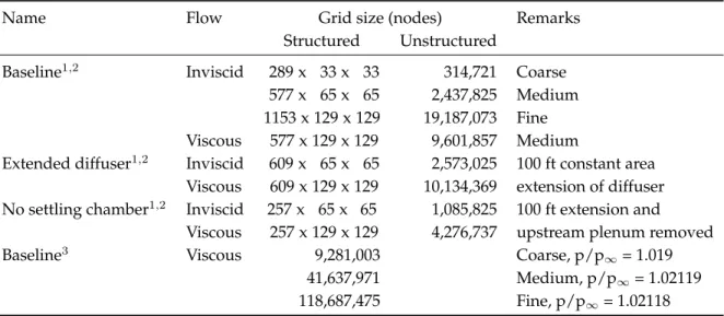
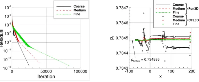
Solution convergence and quality for a sequence of grids using CFL3D and FUN3D are shown in Figs. 13 and 14. Iterative convergence was attained for all three grids using both codes; results are shown for FUN3D in Fig. 13(a). Both codes predicted deviations in the tunnel centerline total pressure, Fig. 13(b), indicating inadequate grid resolution in the contraction section of the upstream settling chamber. The consistency of total pressure greatly improved with grid refinement. Centerline Mach number distributions for CFL3D and FUN3D in the region of the tunnel test section are shown in Fig. 14(a). Similar to trends that have been observed in other studies,33 _{CFL3D approached the} grid-converged result from “above” while FUN3D approached from “below.” With three grid levels of grid refinement, Fig. 14(b) shows that the Mach number at tunnel stationx= 17.75ft was trending toward a similar result for the two codes.

(a) Iterative convergence, FUN3D.

x

p

(b) Total pressure conservation, CFL3D and FUN3D.

Figure 13. Solution quality, grid convergence, Baseline tunnel model, inviscid wall BCs, FUN3D and CFL3D.

2. Viscous calculations on the Baseline model

OVERFLOW viscous solutions based on different grid resolutions are discussed in this section. The Roe upwind scheme along with the ARC3D diagonalized Beam-Warming scalar pentadiagonal scheme were used. Full multigrid cycles were used to help initialize the solution and help accelerate the convergence. Solutions were run in the steady-state mode. The Spalart-Allmaras turbulence model34 _{with the rotation-curvature (RC) correction}35 _{and quadratic} constitutive relation (QCR)36_{(SA-RC-QCR2000) were used.}

x

M

a

c

h

(a) Centerline Mach number.

h = (1/N)

Ma

ch

Figure 14. Mach number, grid convergence, Baseline model, inviscid wall BCs, FUN3D and CFL3D.

There is a large corner separation in the diffuser of the coarse grid solution, as shown in Fig. 15(a), that is less pronounced in the two finer resolutions. The centerline Mach number, wallCp, and wallCfx, shown in Fig. 16, are

nearly identical for the medium and fine grids. Low Mach number preconditioning generally improves convergence behavior for these cases. The residual history plots in Fig. 17 shows the residuals for the three grid levels. The residuals all initially drop and then level out. By turning on the preconditioning, the residuals drop an additional1-2orders for the medium and fine grids. However, the large separation on the coarse grid prevents similar improvement on that grid.

Fig. 18 shows upflow angle (tan−1(w/u)) at stationx= 17.75ft on the three grid levels in OVERFLOW. Results indicate only small differences between the medium and fine grids. The upflow angle varies basically in horizontal bands, with higher angle (approximately0.2deg.) above the tunnel bottom wall and slightly negative, near-zero angle close to the tunnel top wall. The corners and walls introduce significant variations, and cause nonuniformities in the horizontal striations.

Tunnel Mach number for the OVERFLOW grid refinement cases were calculated two ways: the wind tunnel method, which calculates the tunnel speed from the stagnation and static probe measurements, and direct query of a point(17.75,0,0)inside the test section. For the wind tunnel method, the stagnation pressure and static pressure were obtained from the sensor points as described in Section IIID. The pressure values were then fed into the same function used by the 14x22 to calculate the test section speed. This calculated tunnel Mach number is compared to the direct probe at(17.75,0,0)in Table 4. The two different methods of calculating the Mach number produced values within 1% of each other. When a model is present in the tunnel, having a method for consistently and accurately duplicating the tunnel conditions in the CFD is important. The wind tunnel method is one way, but making other measurements for corroboration is also desirable. These other measurements might include isolated probes to measure velocity at specific locations away from the model, wall pressures, and diffuser pressures, for example.

Table 4. Calculated Mach number vs. Direct Probe at(17.75,0,0).

Grid Calculated Mach Direct Mach Probe

Coarse 0.2023 0.1995

Medium 0.2029 0.2004

(a) Coarse grid. (b) Medium grid.

(c) Fine grid.

Figure 15. Tunnel flow visualization,uvelocity, viscous wall BCs, OVERFLOW.

G. FUN3D Empty Tunnel Geometry Modeling Studies 1. Inviscid calculations.

Inviscid solutions for the Baseline, Extended diffuser and No-settling chamber geometries are discussed in this section. Results for the three tunnel modeling variations using the FUN3D code are shown in Fig. 19. Iterative convergence was achieved in all instances, Fig. 19(a) and (b). The pressure coefficient distributions on the left wall (pilot’s perspective) were insensitive to geometry tunnel modeling as seen in Fig. 19(c). The slope of the centerline Mach number was significantly different when switching between the tunnel modeling with and without the upstream plenum, as seen in Fig. 19(d) immediately downstream ofx = 0. Fig. 20 shows upflow angle (deg.) atx = 17.75ft for the three inviscid models. Baseline and extended diffuser were essentially the same, while the grid with no settling chamber yielded almost perfectly uniform horizontal contours.

2. Viscous calculations

Viscous results for the three tunnel modeling variations with the FUN3D code and SA-RC-QCR2000 turbulence model, are shown in Figs. 21, 22, and 23. No adjustments were made in the reference and boundary conditions between the various tunnel models, the result being that the computations did not compensate for different degrees

x

M

a

c

h

(a) Centerline Mach number.

x

Ma

ch

(b) Centerline Mach number, test section.

x

C

(c) Pressure coefficients, left wall, test section.

x

C

(d) Skin friction coefficients, left wall, test section.

Figure 16. Grid sensitivity, viscous wall BCs, OVERFLOW.

of viscous loss in the tunnel. As shown in Fig. 21(a), for these cases approximately seven orders reduction in the continuity equation solution was achieved. The total pressure along the tunnel centerline is plotted in Fig. 21(b) as an additional assessment of solution state and convergence. The Baseline and Extended diffuser grid solutions showed a small, but noticeable oscillation in the total pressure through the plenum contraction and into the tunnel test section,

x=−50ft tox= 0. Eliminating the upstream settling chamber removed the error in the total pressure conservation, as shown by the ’dash-dotted’ line in 21(b). Adversely though, the difference between the with- and without-plenum modeling is quite obvious in the tunnel left wall (pilot’s perspective) local skin friction coefficients, Fig. 22(a), where the no-settling-chamber flow has a very high skin friction coefficient value before coming down more in line with the baseline and extended-diffuser grid solutions. The general shape of the pressure coefficient distributions on the left wall was somewhat similar between tunnel modeling concepts; see Fig. 22(b). Similar to what was observed in the inviscid solutions, the absence of the plenum in the no-settling-chamber geometry is again seen in the lack of flow gradient variation nearx= 0in the test section centerline Mach number plot, Fig. 22(c).

The shift in Mach number and Cplevels between the various models can be partially accounted for by the difference in viscous losses associated with each simulation. Complicating the comparisons is that the baseline grid could not be run using the default back pressure boundary condition in FUN3D due to the persistence of separated flow in the corners of the diffuser. A special “blocking” boundary condition was used for the baseline case to prevent reverse flow from destabilizing the solution. When reverse flow is not present at the outflow boundary, the “blocking” condition

(a) Coarse grid. (b) Medium grid. (c) Fine grid.

Figure 17. Solution residuals, grid sensitivity, viscous wall BCs, OVERFLOW.

(a) Coarse Grid. (b) Medium Grid. (c) Fine Grid.

Figure 18. Upflow (deg.) atx= 17.75ft, viscous wall BCs, OVERFLOW.

duplicates the results of the default back pressure condition. When reverse flow is present, the “blocking” aspect, while preventing the solution from diverging, is physically inconsistent. Fig. 23 shows upflow angle for the viscous cases atx= 17.75ft. The baseline and extended diffuser cases were very similar, and were close to the OVERFLOW viscous results shown in Fig. 18 earlier, as well as to the one published in Nayani et al.25 However, the case with no settling chamber yielded nearly uniform striations with very little deviation in the corners. Because the inflow boundary condition for the CFD imposes uniform flow, the computation without a settling chamber provided only a short run upstream ofx= 17.75ft, so the wall boundary layers and corner flow regions were not as developed as the computations that included the upstream contraction.

H. OVERFLOW JF Free-air and In-tunnel Parametric Studies

According to Aeschliman and Oberkampf,4_{uncertainty due to flowfield nonuniformity in wind tunnels can be} signif-icant. In a wind tunnel experiment, the uncertainty due to a combination of flowfield nonuniformity uncertainty and instrumentation uncertainty is computed by comparing measurements made with the model at different locations in the test section, and/or by rotating the model. However, these types of measurements may be challenging in some circumstances, due to limitations of the hardware or perhaps due to limited testing time. In any case, there is now a desire to explore the ability of CFD to help assess flowfield nonuniformity uncertainty.

In this section, we explore the influence of various global modeling decisions on the JF model region of interest. The relative impact of the tunnel walls on the flow are assessed via a simple sensitivity study that examines the effect of tunnel walls and positional variance. The 8% F6 model was chosen for this study. The CFD model is configured with a horn installed on the starboard wing, and no horn on the port wing. However, future tunnel tests with the 8% JF model will be run either with horn or without horn (same configuration on both wings). The following cases were run using OVERFLOW: (1) in free air, (2) at the nominal (center) position in the 14x22, (3) 1 foot up (vertically) in the tunnel, (4) 1 foot right (facing upstream) in the tunnel, and (5) 1 foot up and 1 foot to the right in the tunnel. Unless otherwise indicated, all of these cases were run atα = 5deg.,M = 0.2,Re = 2.4million based on crank chord, using the SA-RC-QCR2000 turbulence model. An additional in-tunnel run was also performed atα= 5.5deg.

Note that this current CFD exercise is a precursor of our eventual plan. Here, the CFD runs in the tunnel still use uniform inflow boundary conditions in the plenum 70 feet upstream of the test section. Although it does not account for any possible flowfield nonuniformities that may be present in the tunnel at that point in the circuit, the

(a) Iterative convergence.

x

p

(b) Total pressure conservation.

x

C

(c) Left wall pressure coefficients.

x

M

a

c

h

(d) Centerline Mach number.

Figure 19. Variation of tunnel modeling, inviscid wall BCs, FUN3D.

plenum geometry and contraction section do introduce considerable asymmetries in the flow by the entrance to the test section, as shown in the empty tunnel simulations. The question is: how big are the flowfield nonuniformities coming into the plenum from the circuit relative to those nonuniformities caused by the plenum geometry and contraction? Traditional CFD simulations of the high-speed leg can presumably model the latter, but have no hope of capturing the former. Therefore, eventually, we would like to introduce flowfield nonuniformities at the CFD inflow boundary that are representative of what is in the real tunnel (as measured, perhaps, by the QWSS or by PIV, as discussed in Section II). Then, the CFD might be useful in helping to characterize the influence of these nonuniformities on flowfield quantities of interest.

Figure 24 shows the OVERFLOW grid for this F6 model. The grid is comprised of 16 zones (4 for the fuselage, and 6 zones for each wing), resulting in a total of 6.4 million grid points. For the free-air case, the F6 grid was embedded in an off-body Cartesian grid, with the far field located ten body lengths away. For the tunnel cases, the F6 grid was inserted into the grid for the as-built wind tunnel. The model was rotated and translated until it was in the desired location with OVERFLOW-D’sConfig.xmlframework.

The baseline case was run with the fine tunnel grid, and the back pressure was modified until the test section reached the desired Mach number 0.2 with the wind tunnel method mentioned in Section IIIF2. The subsequent positional cases were run based off the baseline case. The model was translated or rotated to the desired location, and then restarted from the baseline case. The back pressure needed to be readjusted in almost all of the cases. The

(a) Baseline. (b) Extended diffuser. (c) No settling chamber.

Figure 20. Upflow (deg.) atx= 17.75ft with variation of tunnel modeling, inviscid wall BCs, FUN3D.

(a) Iterative convergence.

x

p

(b) Total pressure conservation.

Figure 21. Solution convergence, variation of tunnel modeling, viscous wall BCs, FUN3D.

results are given in Table 5, and Figs. 25 and 26, which show the side-of-body separation sizes for all the cases. All the measurements were made in TecplotR_{, and have a±0.05inch measurement tolerance. The calculated Mach number}

was taken as the instantaneous value at the end of the run.

The free-air corner separation sizes were slightly longer than those of the tunnel cases, but still had the same overall shape and size. In terms of separation size, there seemed to be very little influence from moving the model in the 14x22. The case with the model moved vertically 1 ft and right 1 ft required a significantly lower back pressure, which may be a result of a larger corner separation in the tunnel diffuser. Bubble sizes were somewhat larger on the side with the horn than on the side without the horn, which is consistent with experimental evidence from the 6% model test.1 _{Iso-surfaces of vorticity are shown in Figs. 27 and 28 for the no-horn side and with-horn side, respectively. The} main thing to note from these figures is that the no-horn side exhibited a very clear horseshoe vortex near the body, emanating from the wing leading edge region, whereas the with-horn side showed no clear evidence of this feature.

To get an indication of the influence of the various modeling differences on details near the region of interest, we extracted some flowfield details in thex= 110inch plane (110inches behind the body’s nose) just upstream of the start of the wing-body juncture separation, as shown in Fig. 29. For the purpose of this exercise, we only looked at the left side of the model (the no-horn side). Typical results are shown in Fig. 30. Here, the nondimensionalv-velocity is plotted, wherevis the spanwise component of velocityin a coordinate system aligned with the model body axis. Results are qualitatively very similar for all three cases. Although not shown, results were also qualitatively similar for other flowfield quantities:u,w,u0_u0_,v0_v0_,w0_w0_,u0_v0_,u0_w0_{, andv}0_w0_{, as well as for results 1 ft up (vertically) and}

1 ft up 1 ft right in the tunnel. (Here, the velocity fluctuation correlation, or kinematic turbulent stressu0

iu0j, is related

to the Reynolds stressτijbyu0iu0j=−τij/ρ.)

x Cf, x -20 0 20 40 60 80 0.000 0.001 0.002 0.003 0.004 0.005 Baseline Extended diffuser No settling chamber

(a) Left wall local skin friction coefficients.

x Cp -20 0 20 40 60 80 -0.2 0.0 0.2 0.4 0.6 0.8

(b) Left wall pressure coefficients.

x Ma ch -20 0 20 40 60 80 0.16 0.17 0.18 0.19 0.20 0.21 0.22

(c) Test section centerline Mach number.

Figure 22. Variation of tunnel modeling, viscous wall BCs, FUN3D.

(a) Baseline. (b) Extended diffuser. (c) No settling chamber.

Figure 23. Upflow (deg.) atx= 17.75ft with variation of tunnel modeling, viscous wall BCs, FUN3D.

rotated usingu=u∗cos(θ)−w∗sin(θ),v=v∗, andw=u∗sin(θ) +w∗cos(θ), where the superscript * indicates the tunnel coordinate system, andθis the angle that the model is rotated (there is no yaw, only pitch angle in this case). The turbulent stresses must also be rotated appropriately, using the following transformation:

   u0u0 u0v0 u0w0 u0v0 v0v0 v0w0 u0w0 v0w0 w0w0   =    cos(θ) 0 sin(θ) 0 1 0 −sin(θ) 0 cos(θ)       (u0u0)∗ (u0v0)∗ (u0w0)∗ (u0v0)∗ (v0v0)∗ (v0w0)∗ (u0w0)∗ (v0w0)∗ (w0w0)∗       cos(θ) 0 −sin(θ) 0 1 0 sin(θ) 0 cos(θ)    (5)

Figure 31 shows the velocity components for all of the parametric variations along a vertical line approximately

0.7inches from the wall juncture in thex= 110inch plane. When using the SA-RC-QCR2000 model, there were only slight differences between the results of all cases, including free air. An additional free-air case using the SA model was also included in these plots, to show that the differences due to turbulence modeling variations were significantly larger than the differences due to the CFD parametric variations. Nondimensional turbulent stresses along the same line are shown in Fig. 32. All six stresses are plotted. For these quantities, the differences caused by the parametric variations were larger than they were for the mean flow velocities, with the free-air case showing noticeable differences from the tunnel cases. However, again the turbulence model itself had the largest impact. Eventually, noting if this is still the case when accounting for the influence of tunnel freestream nonuniformities will be important.

(a) JF F6 grid ISO view. (b) JF F6 grid top view.

Figure 24. JF 8% model, OVERFLOW overset grid.

Table 5. JF side-of-body separation size sensitivity (inches),M= 0.2,Re= 2.4million,α= 5deg.

Case No-Horn No-Horn W-Horn W-Horn Calculated p/p∞

Length Width Length Width Mach back pressure

Free Air 4.48 1.35 5.49 1.66 N/A N/A

Baseline 3.97 1.33 4.78 1.65 0.2007 1.0191

Up 1 ft 4.07 1.26 5.01 1.68 0.2065 1.0191

Right 1 ft 4.03 1.32 4.92 1.68 0.2004 1.0193

Up 1 ft & Right 1 ft 4.08 1.31 4.95 1.70 0.1942 1.0167

+0.5deg. AoA 3.91 1.33 4.95 1.67 0.2011 1.0192

(a) Free Air. (b) Baseline no-horn. (c) +0.5deg. AoA.

(d) Up 1 ft. (e) Right 1 ft. (f) Up 1 ft & Right 1 ft.

(a) Free Air. (b) Baseline no-horn. (c) +0.5deg. AoA.

(d) Up 1 ft. (e) Right 1 ft. (f) Up 1 ft & Right 1 ft.

Figure 26. JF 8% model side-of-body separation size comparison, with-horn side, OVERFLOW.

(a) Free Air. (b) Baseline.

(a) Free Air. (b) Baseline.

Figure 28. JF 8% model iso-surface of vorticity magnitude and surface pressure contours, with-horn side, OVERFLOW.

(a) Free Air. (b) Baseline tunnel. (c) Tunnel, right 1 ft.

Figure 30. Contours ofv/Urefatx= 110inches, near the JF region, OVERFLOW.

(a)u/Uref. (b)v/Uref.

(c)w/Uref.

(a)u0_u0_/(U2 ref). (b)v 0_v0_/(U2 ref). (c)w0_w0_/(U2 ref). (d)u 0_v0_/(U2 ref). (e)u0_w0_/(U2 ref). (f)v 0_w0_/(U2 ref).

IV.

Summary

This paper described a wide range of studies connected to the NASA Juncture Flow (JF) project, all with the common theme of determining and assessing boundary conditions for the JF model in the NASA Langley 14- by 22-Foot Subsonic Tunnel. Of particular interest is the oncoming (upstream) flow entering the test section, since flowfield nonuniformities may play a role in integrated testing uncertainties in the tunnel. Investigative wind tunnel tests that involved the Boeing Quantitative Wake-Survey System (QWSS) and Particle Image Velocimetry (PIV) were summarized. Both methods are currently capable of measuring the inflow near the front of the test section, but not further upstream in the plenum or contraction. The features of each method, as well as some of their pros and cons, were highlighted. However, this paper only provided an overview; additional details will be given in future publications.

Three CFD codes were used to explore boundary conditions and modeling tactics associated with computing the high-speed leg of the 14x22. Solutions using inviscid tunnel walls were obviously less costly and easier to run, but they were limited in terms of their inability to model flowfield features caused by the wall boundary layers, especially near the corners. Viscous wall solutions could be problematic when corner separation was present in the diffuser, but strategies to overcome these issues were introduced. With a model installed in the tunnel, setting the “correct” corresponding tunnel boundary conditions can be challenging for CFD. OVERFLOW made use of measured total and static pressures at specific upstream locations, and iterated on the back pressure. In the future, other measurements such as static pressures in the diffuser should help CFD. Neglecting the settling chamber in the CFD was found to be a poor approximation when the inflow plane used uniform conditions, because such a large region of upstream development was cut off. However, because we may be forced to measure inflow properties inside the test section, if nonuniform inflow is desired for CFD, our only recourse in the near-term will likely be to impose some approximation of a measured nonuniform state at the inflow plane of the CFD near the start of the test section. Future work along these lines is planned.

Finally, some parametric CFD studies were conducted for the JF model, to determine sensitivities of the flow near the wing-body juncture region of the model to a variety of modeling decisions. These variations included free-air com-putations and in-tunnel comcom-putations with the model in different locations. This study was only a beginning, because the CFD could not yet impose realistic nonuniform boundary conditions at the inflow. So the only nonuniformities present were due solely to those resulting from the tunnel high-speed leg geometry itself. With this, the variations yielded only very minor differences in the region of interest. In fact, turbulence modeling by far was the most influen-tial parameter, followed by free-air vs. in-tunnel runs. Future work will include (1) additional assessment of the state of inflow nonuniformities in the tunnel, and (2) applying realistic inflow variations in CFD simulations to determine their impact.

Ultimately, with highly detailed wind tunnel tests geared specifically for CFD validation, we would like to learn enough information so that CFD can unambiguously run “apples-to-apples” comparisons. In this way, lack of agree-ment caused by possible geometric and boundary condition differences will be off the table, leaving only modeling issues as the source. Then, presumably, efforts to validate or improve the CFD models will be an easier task.

Acknowledgment

The authors thank the Boeing QWSS team: Ashley Jones, Larry Kucera, and Bruce Faulkner. Ms. Jones also provided editorial advice. Lead test engineer Ashley Dittberner and her entire 14x22 team are commended for their excellence and dedication. Thanks go to Bill Oberkampf for his insight, advice, and useful discussions. The authors acknowledge Chung-sheng Yao and Mark Fletcher on the PIV team. Many others—including members of the JF Team—also deserves thanks for their important roles in helping to move this project forward. From NASA Langley, these people include: Dan Neuhart, Mike Kegerise, Kevin Disotell, Joe Morrison, Bil Kleb, Cathy McGinley, Mujeeb Malik, Mark Cagle, Sandy Webb, P. Balakumar, Don Smith, Andy Davenport, and Frank Quinto. Others include John Vassberg, Tony Sclafani, Mike Beyer, Neal Harrison, Peter Hartwich, and Philippe Spalart from Boeing; Roger Simp-son and Gwibo Byun from AUR; Aurelien Borgoltz and Todd Lowe from Virginia Tech; Jim Coder from University of Kentucky; and James Bell, Greg Zilliac, Nettie Roozeboom, and Laura Simurda from NASA Ames. This work was supported by NASA’s Transformational Tools and Technologies (TTT) project of the Transformative Aeronau-tics Concepts Program, and the AeronauAeronau-tics Evaluation and Test Capabilities (AETC) project of the Advanced Air Vehicles Program.