Economics Working Paper Series
2020/016
The Roles of Faith and Faith Schooling in
Educational, Economic, and Faith Outcomes
Andrew McKendrick and Ian Walker
The Department of Economics Lancaster University Management School
Lancaster LA1 4YX UK
© Authors
All rights reserved. Short sections of text, not to exceed two paragraphs, may be quoted without explicit permission,
provided that full acknowledgement is given. LUMS home page: http://www.lancaster.ac.uk/lums/
The Roles of Faith and Faith Schooling in
Educational, Economic, and Faith Outcomes
Andrew McKendrick
aand Ian Walker
bAugust 3, 2020
Keywords: Religiosity, faith schools, educational and long-term outcomes, faith persistence
JEL codes: I21, Z12
Abstract:
We examine the effects of intrinsic religiosity and faith-based schooling on short and longer-term outcomes among young people in England. Without an obvious quasi-experimental identification strategy we rely on a detailed dataset, a cohort study from England with an extensive range of household and school-level characteristics, to use Ordinary Least Squares (OLS), augmented by the Oster (2019) test. Inverse Probability Weighting and mediation analysis are also employed. We show that an individual’s intrinsic religiosity is an important driver of short-term educational outcomes (age 16 test scores) and some longer-term outcomes (later Christian belief), while faith-based schooling plays a lesser role.
Acknowledgements: McKendrick was supported by a PhD studentship from the Economic and Social Research Council, while Walker was supported by a grants from the ESRC and the Nuffield Foundation that were concerned with wider school choice issues. We are grateful to participants in seminars at Lancaster University, and to Derek Neal, Olmo Silva, Jack Britton, Damon Clark, Emma Gorman, Giuseppe Migali, Maria Navarro Paniagua, Vincent O’Sullivan, and Anwen Zhang who gave helpful comments at various events. We are grateful to the Centre for Longitudinal Studies (CLS) at UCL’s Institute of Education, and to the UK Data Service for making available the Next Steps and NPD data. However, neither CLS nor the UK Data Service bear any responsibility for the analysis or interpretation of these data.Access to the data is controlled by the UKDS after registration, application and training. Contact us (a.mckendrick@lancaster.ac.uk) if you require help and guidance with this process, or to access our code.
a. Lancaster University, contactable at a.mckendrick@lancaster.ac.uk b. Lancaster University and IZA, contactable at ian.walker@lancaster.ac.uk
1
1
Introduction
There is a widely held view, among policy makers and parents alike, that faith-based schooling generates superior academic outcomes relative to the alternatives. In many countries faith schools are part of the private or charitable sectors and charge fees; in contrast, in England, faith schools are almost entirely state-funded and cannot charge fees. Faith schools must follow non-faith state schools in delivering the National Curriculum; their funding arrangements are closely comparable, with money following pupils; the requirements for teachers are the same (though faith schools are allowed to use faith as a criterion in hiring decisions); and both are regulated by the Office for Standards in Education (OFSTED). There is much greater comparability between faith and non-faith schools in England than there is elsewhere1.
Of the state secondary schools in the England, 18.7% are faith schools a substantial portion of the education system for students aged 11 to 16 (Andrews and Johnes, 2016). Faith schools are popular, generally oversubscribed, and not just for those with religious belief; although faith schools can discriminate by faith in admissions to some extent. Around 20% of those pupils who attend faith schools have no religion or say their religion is of no importance to them. In contrast, approximately 60% of pupils in secular state schools say the same.
A simple comparison of the academic attainment of those in faith schools, compared to their secular equivalents, generally supports the view that they secure better pupil outcomes. Progression to an academic track post-age 16 in England is driven by performance in national exit examinations known as General Certificate of Secondary Education (GCSE). The usual benchmark by which both schools and students were judged was the attainment of at least five “good” grades at GCSE; with “good” being defined as achieving a grade between A* and C, where C is traditionally thought of as a pass.2 In England, recent evidence (Andrews and
Johnes, 2016) has shown faith schools average over 60 percent of pupils meeting that benchmark, compared to 57.4 percent in other state schools.
The impact of faith schools has been addressed extensively in the economics of education literature. What has not been examined (to the best of our knowledge) is the extent to which an individual’s intensity of belief (a measure of intrinsic religiosity) could account for the impact
1 See Long, Danechi, and Loft (2019) for an up-to-date summary of English faith school distinctiveness and how this might
become more distinctive in the future. In the US, faith schools are increasingly covered by school choice programs that include vouchers, tax credit scholarships, and education savings accounts that can be used to offset private school fees.
2 This A*-C grade benchmark applies to the cohort for whom we have data. Since 2017 a new grading system that uses numbers
2
that faith schools have, if indeed they have one. When it comes to the identification of causal effects it is obvious that issues will arise because pupils do not randomly select into the type of school they attend. Bias resulting from selection on unobserved characteristics3 is easy to
imagine in the context of both religious belief and faith school attendance. In the English case, no quasi-experimental method suggests itself, which is not uncommon in the literature. Altonji, Edler and Taber (2005b) argue that no satisfactory instrument exists for estimating the impact of faith schools and instead they develop a method to establish the sensitivity of estimates to selection on unobservables. This method (also referred to as AET hereafter) was later expanded upon and formalised by Oster (2019) and it is this version of the test that we apply here. The approach is well-suited to the particularly rich dataset that we have. Alongside this we use Inverse Probability Weighting Regression Adjustment (IPWRA), which models treatment and outcome separately (see Imbens and Wooldridge (2009)). In addition, we attempt to identify the pathway by which faithfulness and faith schooling are impacting outcomes using non-cognitive skills as mediators along the lines of Acharya, Blackwell, and Sen (2016).
The contribution of this paper is to explore the extent to which pupil outcomes are driven by the type of school they attend or by their own religiosity, defined as the intensity of their belief (rather than their affiliation or participation). We also contribute by examining longer-term outcomes including university attendance and religious belief at age 25. Finally, we continue the tradition in this literature of applying methods that are not robust to selection on unobservables but, instead, rely on testing for the potential bias from such selection. We provide lower bounds to effect sizes, conditional on particular assumptions, using the test developed from AET by Oster (2019).
This paper uses a powerful English dataset to attempt to answer these questions. The dataset combines administrative data from the National Pupil Database (NPD) for all children in all schools in England, with detailed survey data from Next Steps – a cohort study that began in 2004 comprising 15,770 individuals in its first wave. The survey randomly drew 21000 individuals age 13 or 14 (year group 9 of 1 at age 4/5 to11 at age 15/16 in the English system) from around 650 randomly selected English secondary schools and interviewed them each year, over seven waves, until they were age 20. A further, eighth, wave was conducted in 2015 when the respondents were age 25 and a further wave is planned at age 31. Next Steps is similar in
3 Walker and Weldon (2020) conduct an extensive examination of the operation of the school choice mechanism. The
mechanism is blind to prior ability (national test scores are conducted at age 11) with the exception of a very small number or remaining “grammar” schools that do select by prior ability. Although Faith schools are allowed to ask for further information from parents, that might facilitate cherry picking, the authors find no evidence that they do.
3
character to the well-known US National Longitudinal Survey of Youth (NSLY) – although it only contains a single cohort.
The findings are clear. Being faithful (having higher intrinsic religiosity) at age 14, compared to being not being faithful at the same age, is associated with higher attainment at GCSE, and with a greater likelihood of having a religious belief at age 25 – results that we show to be robust to unobserved confounders. Individual attainment in the national Advanced Level (A-level) examinations at the end of high school, around age 18, and university attendance are also significantly affected by religious belief, though these are less robust. Other outcomes such as: attending one of the more prestigious, so-called Russell Group, universities; university degree class; and the wage rate at age 25 do not appear to be significantly affected by faith. In contrast, the impact of faith schools seems to be much more equivocal. There is a suggestion that faith schools are effective at helping their pupils attain the five GCSE benchmark, but no other outcomes appear to be significantly impacted - except later religious belief. This raises questions as to why parents choose faith schools, which are examined in section 5.6.
The effectiveness of private, faith-based, education has become a more important issue in several countries. Our context is well suited to considering the impact of faith schooling when its provided free. In the US, a recent Supreme Court judgment suggests that tax dollars can now subsidize private schooling (which is often faith-based). In England, the government has committed to expanding existing faith schools and creating new ones, although a large minority of all publicly funded schools are already faith schools. Funding for such schools in England is equivalent to a US voucher that covers the entire costs.
The paper proceeds as follows. The relevant literature is outlined in section 2; the institutional setting and data description in section 3; the empirical strategy in section 4; and the results in section 5. Section 6 concludes.
2
Literature
This paper contributes to two distinct areas of literature – the faith schooling literature in educational outcomes, and the smaller literature on the impacts of religious belief. The faith school literature is extensive but is focussed on Catholic schools in the United States4. Much
less is known beyond this. A number of papers have brought a range of (arguable) instruments to bear on the identification question. Hoxby (1994) uses an area’s Catholic population as an
4
instrument for the presence of a Catholic school and finds a positive impact on area-wide achievement. Noting that exam-based attainment may mean little to some students, Evans and Schwab (1995) examine the impact of Catholic school attendance (at high school level) on both the probability of completing high-school and the probability of going to college. They use Catholic religious affiliation as an instrument for attending a catholic school. Though they go to some lengths to outline the validity of this approach, it is one that the literature as a whole no longer considers to be valid (see Altonji, Elder, and Taber (2005a) discussed below). Correspondingly, Neal (1997) instruments Catholic school attendance with Catholic population density and the density of Catholic schools in a particular area to find a positive impact on wages of attendance at a Catholic school for urban minorities, a small effect for urban whites, and no discernible effect for suburban whites. Kim (2011) conducts very similar work and finds similar effects. The interesting element of the latter paper is that the data contains measures of school quality and that these explain large parts of the Catholic school effects (teacher quality being particularly important). These approaches have been criticised for their potential lack of validity. Neal’s paper specifically is critiqued by Cohen-Zada and Sander (2008) who when replicating his work using different data find Catholic school effects are attenuated substantially by the inclusion of controls for religious affiliation.
Perhaps more convincingly, West and Woessmann (2010) and Allen and Vignoles (2016) each employ the historical religious population of an area as an instrument for the presence of a faith school in that area. The former finds a positive effect and the latter finds little evidence of an impact. However, if culture and values are persistent then the historical population in an area may still affect outcomes through wider cultural mechanisms rather than through religiosity. This could make the instrument invalid. Controversially, Carattini et al. (2012) use Catholic sex abuse scandals in the US as an instrument for the likelihood that an individual is enrolled in a Catholic school. The effect of Catholic school enrolment on public school test scores is then examined to judge if competition from Catholic schools implies better test scores; it does, suggesting that those schools themselves are better performing.
More broadly, Altonji, Elder, and Taber (2005a) argue that there is no convincing exogenous variation that would facilitate analysis of the impacts of faith schools. Though validity of instruments cannot be tested per se, the authors explore a number of routes to cast doubt on the instrumental variable strategies used in the literature. Instead they use data on public school eighth graders, few of whom attend Catholic school, to find a strong link between Catholic religion and educational attainment. In addition, they employ their own innovative method used
5
in their earlier work, that was ultimately published as Altonji, Elder, and Taber (2005b). The method uses the degree of selection on observables to infer the potential impact of unobserved selection (this was later formalised by Oster (2019)). Through it they find a positive impact of Catholic schools on the likelihood of attending university. A range of papers have employed this method, for example Cardak and Vecci (2013) also find small benefits of Catholic schools in terms of the likelihood of attending university.
A further contribution comes from Gihleb and Giuntella (2017) who exploit the rapid decline in the supply of teaching nuns lead to widespread closures of Catholic private schools following Vatican II (1962-1965) - a process of spiritual introspection and renewal for the Roman Catholic church. This is more convincing that early IV attempts because it exploits spatial and temporal variation and they find no effect on grade repetition, contrary to their OLS results. Interestingly, they use the AET method to examine the robustness of the OLS results and find that even a small degree of selection on unobservables is sufficient to drive the OLS results to zero, confirming their IV results.
Chingos and Peterson (2015) find that winning the New York City scholarship lottery had no
overall impact on the college enrolment of students as a whole, but it did have positive impacts for students of color. Much of the effect was associated with Community College enrolment. The effects were larger for Catholic schools that other private schools.
Importantly for the English context, Gibbons and Silva (2011) argue that no credible instrument exists for attendance at a particular type of school. Given this, they use a number of techniques to analyse the impacts of faith schools. They combine their detailed dataset with prior subject-by-achievement-level fixed effects and home-postcode fixed effects; they then exploit the fact that selection occurs twice in choosing faith schools – at both primary and secondary level – to use secondary-type-by-postcode fixed effects to account for family and individual characteristics assuming selection at both secondary and primary level are comparable. If selection into secondary school type is driven by performance in primary then this method will be flawed – so the authors compare those who stay in a faith school between primary and secondary to those who stay in a non-faith school (the faith and non-faith stayers), and compare those who switch between the two types (the switchers). Assuming positive selection into faith schools the stayers will provide an upper bound of the faith school effect and the switchers a lower bound. Switchers are found to have virtually no effect and stayers a small positive effect. Finally, the authors implement the Altonji et al method to find that for stayers the moderate effect vanishes even if it is assumed that there are only modest degrees of unobserved selection.
6
Non-cognitive outcomes have also been examined. In the US, Elder and Jepsen (2014) find, using OLS, propensity score matching, and the Altonji et al method, little evidence of an impact on non-cognitive skills (along with a negative effect of Catholic schools on achievement in mathematics tests). Following the same approach Nghiem et al. (2015) find no effect of faith schooling on cognitive or non-cognitive skills in Australia. Their range of non-cognitive skills and controls is extensive which adds weight to their research even in the absence of a more conventional identification strategy. A number of papers also observe a positive relationship between Catholic school attendance in the US and subsequent religiosity (e.g. Sander (2001), and Wadsworth and Walker (2017)) and the notion that parents may explicitly send their children to faith schools in order to improve the likelihood that their child remains religious. A recent report by Andrews and Johnes (2016) makes clear that the backgrounds of those attending faith schools do differ to those of students attending non-faith schools. Faith schools take fewer students from disadvantaged backgrounds (as measured by the proportion of pupils in receipt of free school meals), fewer students who have Special Educational Needs (SEN), and students who are already academically more able. Besides this, other unobserved characteristics exist that make pupils at faith schools different from those at non-faith schools. Turning to religiosity, Hungerman (2014a) discusses religion in the context of club goods. Individuals can have the option of religious consumption and secular consumption. The presence of potential free-riders who want salvation without necessarily conforming to certain practises and rules leads religious groups to emphasise certain behaviours to screen out the unfaithful. These behaviours may include hard work which has implications for educational attainment and labour outcomes. McCullough and Willoughby (2009) similarly suggest that religion modifies an individual’s priorities so that they want to accord with the prescribed practices. The promotion of honest toil and good behaviours would fit the educational context. Endogeneity pervades the empirical analysis of the economic impacts of religion. Self-selection means that a particular kind of person could choose to be religious but would, in the absence of their belief, still perform better in the education system. Reverse causality too has been evidenced in compulsory schooling research in Canada and Turkey (Hungerman (2014b) and Cesur and Mocan (2018) respectively). Finally, the effect of education on religion may not be present for all faiths equally (McFarland, Wright, and Weakliem, 2011) – hence we decompose results between Protestants and Catholics below.
7
Some work claims to identify exogenous variation. Gruber (2005) innovated the religious market density instrument that employs the share of people of the same religious background in a particular area as an instrument for an individual’s religiosity. It is not difficult to imagine spillovers that would make this instrument invalid.
Along more historical lines, Becker and Woessmann (2009) investigate whether a Protestant work ethic resulted in greater levels of economic prosperity in the 1500s. Using distance to Wittenberg (the epicentre of Lutheran Protestantism) as an instrument for Protestant belief there is found to be a positive and significant impact on literacy. In order to read the Bible, one has to be able to read which leads to other economic developments. Similarly, Spenkuch (2017) uses a 1555 treaty to engineer a fuzzy regression discontinuity design (RDD). Serfs followed the faith of their territorial lord (either Catholicism or Protestantism) creating a patchwork of religious populations that correlates strongly with the situation today. Protestants are found to be more likely to work longer hours, and though they do not earn higher wages, they earn more as a result of being paid for more hours of work. Evidently these instruments, though convincing, are not available for use in the setting of English schools from 2004 onwards. Evidence is not limited to the Protestant case. Oosterbeek and van der Klaauw (2013) and Campante and Yanagizawa-Drott (2015) each use the timing of Ramadan to find a negative impact of religious practise on individuals’ test scores in the case of the former and a nation’s economic growth in the case of the latter. However, happiness is found to improve in the latter in accordance with the Hungerman (2014a) club good definition. The implications of this are unclear. The Becker and Woessman result does not have its origin in belief, but in an almost incidental need for literacy. The Spenkuch result points more clearly to religion, whilst the Ramadan-based work ultimately suggests an effect resulting from (a temporary decline in) nutrition, albeit among those with strong enough religiosity to adhere to the practice.
Other work also suggests a role for belief. Focusing on work ethic in an ordered probit analysis, Schaltegger and Torgler (2010) find Protestant faith is still statistically significant when interacted separately with both education and with intensity of religious belief within the same specification. Lehrer (2004), in the context of a model of supply and demand for education finance, finds conservative Protestant women who attend church regularly complete almost one additional year of schooling compared to the less observant.
At the intersection of these two literatures are those papers that examine religiosity and faith schooling effects together. As Cohen-Zada and Sander (2008) point out, there are studies that
8
control for religious affiliation in the estimation of Catholic school effects, though many do not control for religious groups other than Catholics. A UK-focused paper that does explicitly control for religiosity as part of its research quest ion, and is thus close to ours conceptually, is Sullivan et al. (2018), who examine the long-term impact of faith schooling whilst controlling explicitly for the individual’s faith of upbringing.
Using the British Cohort Study (BCS) they are able to look at the long term achievement effects of faith schools and (affiliation-based) religiosity. They find effects of faith schooling and of religiosity on a range of outcomes. As this is close to what we propose it is worth articulating our contribution relative to Sullivan et al. Our measure of religiosity is different – intensity of belief instead of affiliation based. Especially in the context of faith of upbringing, wider cultural factors could be involved beyond religiosity. Our data provides a rich range of other school characteristics from administrative data to control for aspects of faith schooling that the Sullivan et al analysis does not. And, as the authors point out, their setting is schooling in the 1970s and the effects on the individual’s examined at age 42. Hence our setting contributes to the literature by providing a more recent analysis (from 2004) and shows the short to medium-term impact of faith schooling and religiosity instead of the long-medium-term effect.
A second paper that is close to ours is Adamczyk (2009) who uses the same religiosity measure as we have (intensity of belief, along with frequency of prayer and religious practise), and an indicator of Catholic school attendance, to estimate the impact of religiosity on the likelihood that a woman has had a premarital abortion in the United States. Neither religiosity nor religious practise have a significant impact, although being a more conservative Protestant does. Having more conservative Protestant peers has an impact but attending a religious school does not. The paper uses a hierarchical logistic regression that will be vulnerable to omitted variables. The range of controls are not as rich as contained in our paper, and the methodology does not address the robustness of the estimates reported.
Besides the papers above, there is evidence of religiosity impacting health and risky behaviours (Mendolia, Paloyo, and Walker, 2019); voting behaviour (Spenkuch and Tillmann, 2018); and the likelihood an individual pays their taxes (Torgler, 2006). We have not located any previous papers in the faith schooling literature that control for the intensity of belief. Neither is there existing work that matches our broad set of outcomes or provides such a rich range of controls.
9
3
Data
3.1 Institutional Background
3.1.1 Faith Schools
Religious institutions have been involved in English education for centuries - since the earliest schools were established. Historically, these schools were organised and run by religious institutions such as monasteries, and they were private in the sense that they were not maintained by the state even if they did not charge for the provision of their services. The 1902 Education Act brought free, compulsory, and Christian education for all to England, and most schools became part of the state-maintained system. This continued under the 1944 Education Act where faith and non-faith schools became distinct tracks of school (Department for Children, Schools and Famililies, 2007).
Faith schools at the time of the Next Steps cohort are generally voluntary controlled (VC) or voluntary aided (VA). In a VC school a religious body has influence in how the school is run but the school is mainly managed by the local authority (LA). In the VA case a religious institution may hold a stake in the buildings the school inhabits (or even own them completely) and have some small financial involvement in the school’s operation. The religious body will also have a majority on the school’s governing body (New Schools Network, 2015). More Church of England schools are VA than VC, while Catholic Schools are exclusively VA.5 A faith school in England is any that has an explicitly stated religious character. Whilst every LA in England has at least one faith school, there is a high degree of heterogeneity between LAs with nine LA areas in England having around 40% of their pupils in faith schools (Andrews and Johnes, 2016). Faith schools are allowed to use religious belief as a criterion for admitting pupils, for up to half of their pupils, if they are oversubscribed. Schools can be of a number of different denominations but the overwhelming majority are Christian. Of these, the lions’ share are Roman Catholic (9.4% of all schools), with a smaller number being Church of England (6.1%) or of other Christian affiliation (2.3%). Jewish schools have existed since 1732, Muslim schools since the 1950s, and Sikh and Hindu schools since 1999 and 2008 respectively. Crucially, as regards the ethos of a particular institution, or of the people who staff it, faith schools are allowed to apply religious criteria in their hiring processes. In practise, this means
5 After the growth of Academy Schools and the inception of Free Schools, which are both state funded but independent of
local authorities, the picture has become more fragmented. At the time of the Next Steps cohort, though, there were relatively few secondary academies and there were no Free Schools.
10
being able to choose one person over another if that person’s beliefs align with that of the school. They also have freedom over what they choose to teach in Religious Studies classes, a GCSE level subject taught widely in schools but is outside of the National Curriculum. It is clear that what is meant by a faith school in the context of England is distinct from what would be meant in the US context. In the US, Catholic schools are usually not public funded and operate very differently to an English faith school.
3.1.2 Key Stages
Children in the UK attend primary school from the ages of 4 or 5 up until age 11. Secondary schooling follows from ages 11 to 16. This applies to all students, and stratification occurs post-16 with the option to go into vocational training, as part of an apprenticeship scheme or full-time, or further academic studies.6 Within primary and secondary schools, students are organised into ‘Key Stages’ (KSs). These are referred to as: KS1, which covers ages 5 to 7 (years 1, 2, and 3); KS2, which covers ages 8 to 11 (years 4, 5, and 6); upon moving to secondary school, ages 12 to 14 (years 7, 8, and 9) fall into KS3 with ages 15 to 16 (years 10 and 11) and 17 to 18 (years 12 and 13) belonging to KS4 and KS5 respectively. The Next Steps data covers KS3 onwards with some KS2 characteristics available.
At the end of each of these stages there are tests or national exams; GCSEs are completed at the end of KS4 and constitute the exit examinations from secondary schooling, whilst KS5 ends with the A-Level national examinations. KS5 is far narrower than the earlier KS levels with the typical student taking just three or four subjects. In contrast, KS4 normally includes 7-10 subjects with limited electives; 5 passing grades, usually including maths and English, are required to pursue an academic track, post-age 16, at KS5. One’s A-level subjects, and the grades attained, determine access to undergraduate courses in universities.
3.2 Next Steps Data
This paper uses the Next Steps dataset (also known as the Longitudinal Study of Young People in England (LSYPE)).7The dataset is a cohort study beginning in 2004 with the sampling of
approximately 21,000 Year 9 (KS3) pupils from 647 English State and Independent
6Since 2015 young people in England born after 1997 have had to stay in some form of education up until the age of 18. This
does not apply to the Next Steps cohort, the overwhelming majority (99.8 percent among first wave participants) of whom were born in 1989 and 1990. As such, the Next Steps cohort face a leaving age of 16.
7 The data and documentation can be found at University College London (2020). A full description of the dataset and its
11
paying) schools.8 Questions were then asked of both the cohort member and their parents. In the first wave 74 percent of those contacted responded, yielding a sample of 15,770. Waves two to seven have response rates in excess of 85 percent (with the exception of the ethnic boost sample in wave 4 that has a 59 percent response rate). This represents a low level of attrition. The study followed the cohort member (aged 13 or 14 in wave one) through their remaining years of education and up until the age of 20. The study then stopped until it was resurrected by the Centre for Longitudinal Studies for an eighth wave in 2015. This enables the same individual to be observed from age 13 to 25 and allows analysis to cover the impact of religiosity at an early age on later life outcomes. Whilst waves two to seven only include people who responded to the previous wave, wave eight saw all initial members (i.e. those who responded to wave 1) contacted and an ultimate sample size of 7,707 individuals (51 percent response) was achieved. We dropped from the wave one sample those who declared they were not Protestants, Catholics or of no religion. The numbers who declared themselves to be Muslims or to belong to other religions were too small to allow meaningful analysis, and only a small percentage of such people attended faith schools in our data.
This paper primarily makes use of Next Step's first wave (where respondents are 13 or 14 years old) with outcomes appearing from the eighth wave and some potential mediators coming from the second wave. Variables relating to religiosity, gender, ethnicity, and parental characteristics come exclusively from the first wave. Wave eight is used for information regarding university attendance, income, and other labour market outcomes. The sixth and seventh waves are used only to provide information on university attendance for those who were not present in wave eight. The outcome variables of interest are test scores at various different key stages, university attendance and performance, and the wage rate earned at age 25, eleven years after the faithfulness questions are asked. Christian affiliation at age 25 is also recorded.
In terms of test score outcomes: attaining the five A*-C grades benchmark is a binary outcome;
number of GCSE passes is ordinal; and the GCSE point score is more granular and is calculated by attaching a score to each grade attained.9 A-level attainment is measured by the University and College Admissions Service (UCAS) equivalent point score for the top three grades attained (even if more than three subjects were taken).10 The UCAS score is used by universities
8 In our analysis we examine state-maintained schools only.
9 At GCSE, A* is worth 58 points, A is worth 52, B is worth 46, decreasing by 6 points until a grade G which is worth 16. 10 For A-levels, when converted to UCAS points, A* is worth 140, A is worth 120, B is worth 100, C is worth 80, D is worth
12
when they review applications; focussing on the top three subject studied means that somebody who attained an A and three Bs does not appear to be performing better than somebody with three As. But the person with three As would, in practise, be much more likely to be accepted by a “better” university than the mostly-B-grade achieving student. We standardise both the GCSE point score and UCAS A-level point score.
The later, post high school, outcomes are defined as follows: university attendance is a binary variable taking the value one if the individual attended university by the time they were aged 25; Russell Group university attendance is a binary outcome indicating whether an individual attended one of the more prestigious research-intensive universities in the UK; degree classification is a binary variable that takes the value one if the individual was awarded a first class or upper second class degree at university and 0 otherwise (around ⅔rd of this cohort will
have attained such a “good” degree). The wage rate is the log of labour income (in the individual’s main job) divided by the number of hours worked per week in that job. Christian belief at age 25 is a binary variable that takes value one if the individual identifies as Christian in wave eight.
The Next Steps dataset is linked to the National Pupil Database (NPD). This is the government’s administrative dataset for education in England.11 This gives access to the
academic achievement of the individuals in the Next Steps cohort and allows the denomination of the school the individual attended to be identified (i.e. faith versus non-faith). Additionally, a broad collection of school level characteristics are available, such as the ethnic mix of the school and the percentage of children eligible for free school meals (FSM), a proxy for lower socio-economic status.
Also available is the index of multiple deprivation (IMD) which measures the socio-economic status of the neighbourhood in which the cohort member lives, down to the postcode level (an average of 15 households). The multiple deprivation measure incorporates local levels of variables such as income; employment; health and disability; education, skills and training; barriers to housing services; and living environment and crime levels. Altogether, the available set of controls is extensive and suggests that a higher proportion of selection might be observed and explained than would be the case for other datasets.
11 Education is a “devolved” policy area in the UK meaning that each nation within the United Kingdom has control over its
13 3.3 Measuring Religiosity
Religiosity is measured in Next Steps in accordance with recommendations made in McAndrew and Voas (2011). Three different facets of belief are covered: affiliation (or
extrinsic religiosity); belief (or intrinsic religiosity, which we refer to as faithfulness in this paper) which we derive from the religion’s importance in one’s life question; and practise, which we derive from in the questions relating to participation in religious classes. The precise questions are given in Appendix Table A1.
The primary religiosity measure in this paper is 'faithfulness' or 'intrinsic religiosity', as it is often referred to. We use faithfulness throughout to more concretely refer to the treatment of interest, since intrinsic religiosity could easily, and confusingly, refer to other measures of practise (e.g. religious class attendance) as well as belief. Our faithfulness variable is the individual cohort member's response to the question: 'How important would you say your religion is to the way you live your life?' with four potential answers: "Not at all", "Not very", "Fairly" and "Very" faithful.
In the survey, those without a religion are not asked the faithfulness question, and are therefore coded here as not at all faithful. This variable is arguably superior to other measures of religiosity that are often used – variables based on affiliation and practise. For example, in a notionally Christian country, an individual may self-report being a Christian in survey data when, in practice they are not. Similarly, a young person may be taken to church by their parents but neither wish to be there nor care about what they hear whilst there. Thus, our definition, although subjective, does reduce a more explicit form of measurement error that could otherwise occur.
3.4 Descriptive Statistics
There are two treatments of interest – faithfulness and faith schooling. Additionally, interaction effects are examined later. If the faithfulness variable is kept as is, with four categories and with the separate faith school treatment then there will be four coefficients of interest (seven in the interaction case). This is arguably too many, since cell-sizes begin to get too small, to support precise estimates of the interaction treatments. Moreover, the Oster (2019) test, outlined below, is designed for binary treatments. We, therefore, collapse the three faithfulness treatment levels above the lowest into one, leaving a binary treatment that is 0 if the individual is not faithful, and 1 if the individual is faithful. Pairwise tests of coefficients each of the four
14
faithfulness levels (not shown) suggest that this is reasonable, with few statistically significant differences.
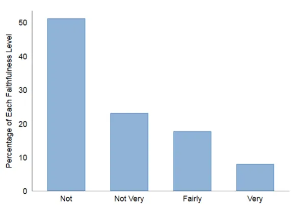
Figure 1 shows the percentage of each faithfulness level in the data, before the it is collapsed to binary. Figure 2 shows the way that faithfulness is broken down by Christian denomination and by Faith and Non-Faith School attendance. Those of no religion are, by construction, classified as not at all faithful. There are clearly more Protestants who are of lower faithfulness than there are Catholics of lower faithfulness. The same is true of non-faith schools relative to faith schools, as would be expected, with over half of non-faith school attendees being not at all faithful.
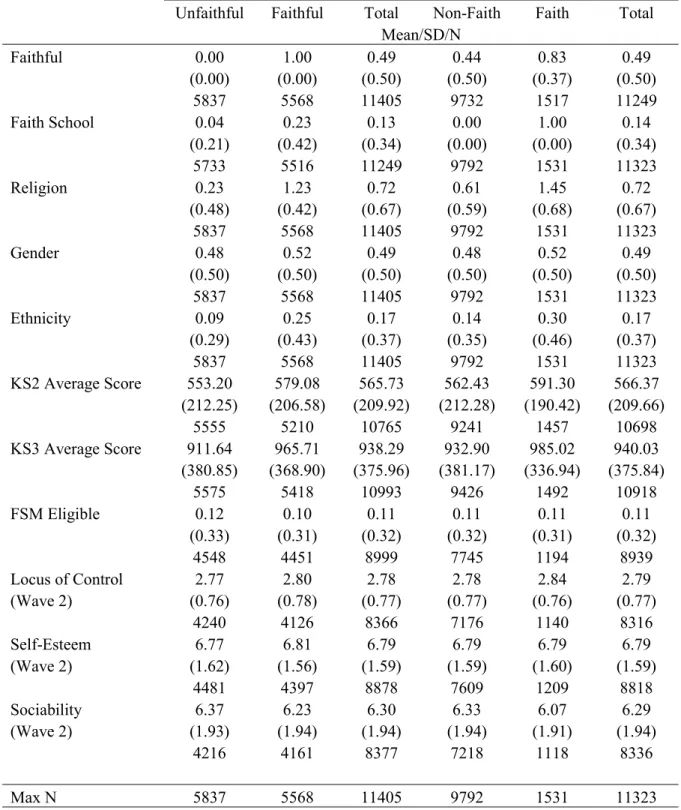
Table 1 shows summary statistics of cohort member’s characteristics and Table 2 shows the outcome variables, broken down by faithfulness and school type.12 The percentage of pupils on free school meals is very similar across all categories as are non-cognitive skills. Those attending faith secondary schools performed better at KS2 (i.e. at primary school), as did the faithful.
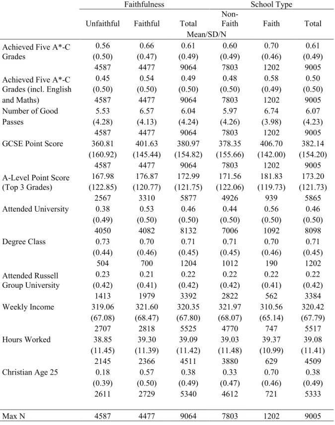
In Table 2 the faithful perform better in all of the schooling outcomes, but there are very small differences in the later outcomes, except for being a Christian at age 25 where there is a very large difference. There are also difference by school type in schooling outcomes and while there is a marked positive effect of faith schooling on attending university, there is no difference in university outcomes conditional on attending university. In the raw data, there appears to be a negative effect of faith schooling on income, but not of faithfulness. The faithful also appear to work longer hours per week – something that may reflect an independent effect of religion that has been noted in some previous work and motivates us to focus on a wage rate defined by the hourly rate of pay in analysis later in this paper.
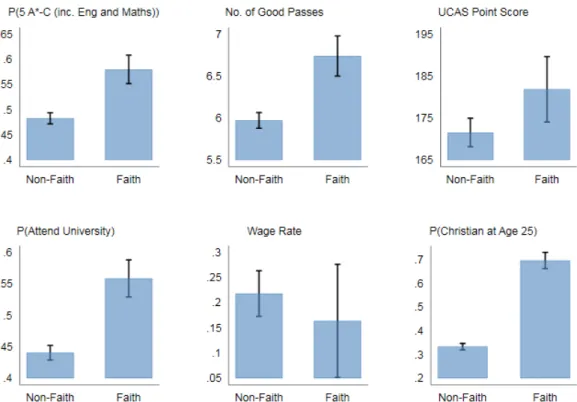
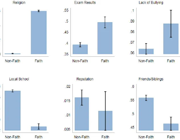
Figures 3 and 4 selected outcome variables broken down by faith school and faithfulness respectively. These support the popular notion that faith schools have better educational outcomes. However, faithfulness shows patterns of effects on outcomes that are very similar to the effects of faith schooling. Figure 4 shows the potential for an interaction effect between faithfulness and faith schooling – there are more faithful individuals in faith schools.
12 Tables A2 and A3 in the Appendix give summary statistics for parental/household characteristics and school level
15 Figure 1 - Distribution of Faithfulness
Note: Displays levels of faithfulness where the survey responses were as appear with the word faithful after: e.g. “Not very” faithful. This is with the exception of “Not” which represents the survey response “not at all faithful”.
Figure 2 - Faithfulness by Religion and School Attendance
Note: Displays levels of faithfulness where the survey responses were as appear with the word faithful after: e.g. “Not very” faithful. This is with the exception of “Not” which represents the survey response “not at all faithful”.
16
Table 1 - Summary Statistics - Individual Characteristics
Faithfulness School Type
Unfaithful Faithful Total Non-Faith Faith Total
Mean/SD/N Faithful 0.00 1.00 0.49 0.44 0.83 0.49 (0.00) (0.00) (0.50) (0.50) (0.37) (0.50) 5837 5568 11405 9732 1517 11249 Faith School 0.04 0.23 0.13 0.00 1.00 0.14 (0.21) (0.42) (0.34) (0.00) (0.00) (0.34) 5733 5516 11249 9792 1531 11323 Religion 0.23 1.23 0.72 0.61 1.45 0.72 (0.48) (0.42) (0.67) (0.59) (0.68) (0.67) 5837 5568 11405 9792 1531 11323 Gender 0.48 0.52 0.49 0.48 0.52 0.49 (0.50) (0.50) (0.50) (0.50) (0.50) (0.50) 5837 5568 11405 9792 1531 11323 Ethnicity 0.09 0.25 0.17 0.14 0.30 0.17 (0.29) (0.43) (0.37) (0.35) (0.46) (0.37) 5837 5568 11405 9792 1531 11323 KS2 Average Score 553.20 579.08 565.73 562.43 591.30 566.37 (212.25) (206.58) (209.92) (212.28) (190.42) (209.66) 5555 5210 10765 9241 1457 10698 KS3 Average Score 911.64 965.71 938.29 932.90 985.02 940.03 (380.85) (368.90) (375.96) (381.17) (336.94) (375.84) 5575 5418 10993 9426 1492 10918 FSM Eligible 0.12 0.10 0.11 0.11 0.11 0.11 (0.33) (0.31) (0.32) (0.32) (0.31) (0.32) 4548 4451 8999 7745 1194 8939 Locus of Control 2.77 2.80 2.78 2.78 2.84 2.79 (Wave 2) (0.76) (0.78) (0.77) (0.77) (0.76) (0.77) 4240 4126 8366 7176 1140 8316 Self-Esteem 6.77 6.81 6.79 6.79 6.79 6.79 (Wave 2) (1.62) (1.56) (1.59) (1.59) (1.60) (1.59) 4481 4397 8878 7609 1209 8818 Sociability 6.37 6.23 6.30 6.33 6.07 6.29 (Wave 2) (1.93) (1.94) (1.94) (1.94) (1.91) (1.94) 4216 4161 8377 7218 1118 8336 Max N 5837 5568 11405 9792 1531 11323
Note: Faithful is a binary indicator, 0 for unfaithful, 1 for faithful; faith school also takes the value 0 for a non-faith schools and 1 for a non-faith school. Religion is coded from 0 to 2, 0 is no religion, 1 is Protestant, and 2 is Catholic; Gender takes value 1 if the individual is female and 0 if male; Ethnicity is 1 for non-white individuals and 0 otherwise; KS2 and KS3 point scores are continuous; FSM eligible takes value 1 if the individual is on free school meals; internal Locus of control goes from 1 to 4 with 4 being the highest feeling of control over one’s life and 1 the lowest; Self-Esteem goes from 1 to 8 and with 8 being the highest self-esteem and 1 the lowest; Sociability also goes from 1 to 8 with 8 being the highest and 1 the lowest.
17
Table 2 - Summary Statistics - Individual Outcomes
Faithfulness School Type
Unfaithful Faithful Total Non-Faith Faith Total
Mean/SD/N
Achieved Five A*-C
Grades (0.50) 0.56 (0.47) 0.66 (0.49) 0.61 (0.49) 0.60 (0.46) 0.70 (0.49) 0.61
4587 4477 9064 7803 1202 9005
Achieved Five A*-C
Grades (incl. English (0.50) 0.45 (0.50) 0.54 (0.50) 0.49 (0.50) 0.48 (0.49) 0.58 (0.50) 0.50
and Maths) 4587 4477 9064 7803 1202 9005
Number of Good 5.53 6.57 6.04 5.97 6.74 6.07
Passes (4.28) (4.13) (4.24) (4.26) (3.98) (4.23)
4587 4477 9064 7803 1202 9005
GCSE Point Score 360.81 401.63 380.97 378.35 406.70 382.14
(160.92) (145.44) (154.82) (155.66) (142.00) (154.20)
4587 4477 9064 7803 1202 9005
A-Level Point Score
(Top 3 Grades) (122.85) 167.98 (120.77) 176.87 (121.75) 172.99 (122.06) 171.56 (119.73) 181.83 (121.73) 173.20 2567 3310 5877 4926 939 5865 Attended University 0.38 0.53 0.46 0.44 0.56 0.46 (0.49) (0.50) (0.50) (0.50) (0.50) (0.50) 4050 4082 8132 7006 1092 8098 Degree Class 0.73 0.70 0.71 0.71 0.70 0.71 (0.44) (0.46) (0.45) (0.45) (0.46) (0.45) 504 700 1204 1012 190 1202 Attended Russell Group University (0.42) 0.23 (0.41) 0.21 (0.42) 0.22 (0.42) 0.22 (0.41) 0.22 (0.42) 0.22 1413 1979 3392 2822 562 3384 Weekly Income 319.06 321.60 320.35 321.97 310.56 320.42 (67.08) (68.47) (67.80) (68.07) (65.14) (67.79) 2707 2818 5525 4770 747 5517 Hours Worked 38.85 39.30 39.09 39.03 39.37 39.08 (11.45) (11.39) (11.42) (11.48) (10.99) (11.41) 2145 2366 4511 3880 629 4509 Christian Age 25 0.18 0.57 0.38 0.33 0.70 0.38 (0.39) (0.50) (0.49) (0.47) (0.46) (0.49) 2611 2729 5340 4612 721 5333 Max N 4587 4477 9064 7803 1202 9005
Note: Outcomes are described in detail on Page 12. Five A*-C, Five A*-C (incl. English and Maths), Attended University, Degree Class, Attended Russell Group University, and Christian at Age 25 are all binary. Each takes value one if the condition is true. Degree class takes the value one if the individual got a first or an upper second class degree, and 0 otherwise. Wage, GCSE point score and A-Level point score are continuous variables. Number of Good Passes is discrete.
18
Figure 3 – Mean Outcomes by School Attendance (Faith vs Non-Faith School) (95% CI)
Note: Chart shows selected outcomes for those who are “Unfaithful” (or not faithful) and “Faithful” individuals. Probability of attaining 5 A*-C grades, probability of attending university, and probability of being Christian at age 25 are all binary; number of good passes, UCAS (A-level) point score, and wage rate are not.
Figure 4 – Mean Outcomes by Faithfulness (Faithful vs Unfaithful) (95% CI)
Note: Chart shows selected outcomes for those who are “Unfaithful” (or not faithful) and “Faithful” individuals. Probability of attaining 5 A*-C grades, probability of attending university, and probability of being Christian at age 25 are all binary; number of good passes, UCAS (A-level) point score, and wage rate are not.
19
4
Empirical Strategy
4.1 Specification
Our analysis begins with an Ordinary Least Squares (OLS) estimation of a linear specification: 𝑌𝑌𝑖𝑖𝑖𝑖= 𝛽𝛽0+ 𝛽𝛽1𝐹𝐹𝑖𝑖𝑖𝑖+ 𝛽𝛽2𝐹𝐹𝑆𝑆𝑖𝑖𝑖𝑖+𝛽𝛽3𝑿𝑿𝑖𝑖𝑖𝑖+𝛽𝛽4𝑺𝑺𝑖𝑖 + 𝜖𝜖𝑖𝑖𝑖𝑖 (1) where 𝑌𝑌𝑖𝑖𝑖𝑖is some outcome for individual i in school s: GCSE attainment, A-level attainment, whether or not the individual attends university, attends a Russell group university, attains a “good” degree class, the wage rate at age 25, and whether or not they are a Christian at age 25. 𝐹𝐹𝑖𝑖𝑖𝑖is a binary variable taking the value zero if the individual says their faith is not at all important in their everyday life, and one if the individual says their faith is more important than that (i.e. not very, fairly, or very faithful). 𝐹𝐹𝑆𝑆𝑖𝑖𝑖𝑖 takes the value zero if the individual did not attend a faith school, and one if they did. 𝑿𝑿𝑖𝑖𝑖𝑖is a vector of controls including gender, ethnicity, religion, parental religion, parental education, parental employment status, and number of dependent children in the household. 𝑺𝑺𝑖𝑖is a vector of school level characteristics of the cohort member. These include the ethnic mix, the share of pupils on free school meals (FSM), whether the school has a single sex intake, is academically selective, and has a “sixth form” (senior high school) attached to it. Standard errors (𝜖𝜖𝑖𝑖) are clustered at the school level as this is the primary randomisation unit for the data sampling. Evidently the set of controls is both rich and varied. Religiosity is measured when the cohort members are aged 13 or 14 – in Next Steps’ first wave. Though the faithfulness question is asked in subsequent waves the analysis is based on the first wave information only. This is to ensure that our measure of religiosity is recorded pre-treatment – if we were to use wave 3 faithfulness, after GCSE high stakes exams have been taken, there may be an issue of reverse causality between attainment and religiosity. As there is no quasi-experimental variation here it makes sense to minimise issues such as this.
Sensitivity analysis in empirical research is traditionally conducted by observing how treatment effect estimates change as additional control variables are included; if there is little movement in the estimated treatment effects then the threat of unobserved selection is said to be low. However, as pointed out in Oster (2019) this may not be enough.13 Hence, we augment the
13 The example, in the introduction of Oster (2019), is the effect of education on wages. There are two orthogonal components
of ability, one that has high variance and the other low variance – if both were included all variation would be explained. Controlling for the low variance ability component would not change coefficient sizes all that much – leading to the conclusion that selection on unobservables was not an issue. But the bias would still exist by omitting the second, high variance, ability control.
20
OLS estimates with the test suggested in Oster (2019). The test extends prior work by Altonji, Elder, and Taber (2005b). Their paper suggested that it might be reasonable to assume that the amount of selection on unobservables could be bounded from above by the amount of selection on observables. If covariates to be included in estimations were picked at random from the full set of possible covariates, selection on unobservables would be less than or equal to selection on observables. As researchers do not pick covariates at random but based on other empirical studies and theoretical justification for their inclusion, in reality selection on unobservables in a rich data set is likely to be less than that which is observed and controlled for. Bounds on OLS estimates can also be produced using their method.
Oster (2019) points out that observed selection is only informative about unobserved selection if the two are distributed in the same way. Assuming that it is in a rich dataset, it will be the case that explaining all variation, i.e. attaining an R2 value of one, is impossible. This is due to
measurement error in research data. As a result, the Oster test provides a procedure to use the observed R2 value from estimated regression specifications multiplied by something larger than
one. Oster suggests, on the basis of comparison of randomised controlled trial estimates with non-experimental estimates from a range of previous studies, that 1.3 would be appropriate. More conservatively, estimates are also provided in the tables below that use double the R2.
The test can be used in two ways – firstly to infer the degree of unobserved selection the that would need to exist to reduce the magnitude of the treatment coefficient to zero. This is the 𝛿𝛿 value. The threshold for robustness in this case is one – equal observed and unobserved selection. The second way is to bound estimates assuming a particular degree of unobserved selection – the 𝛽𝛽 value. The test is not a silver bullet that enables causal inference, but it substantially augments the usefulness of OLS estimates in that it may allow researchers to argue selection bias is unlikely to bias estimates substantially.
It is useful to articulate the nature of the expected omitted variable bias. The most obvious is likely innate ability. For example, in Table 1 the faithful and those attending faith schools have higher KS2 scores than the unfaithful and those in secular schools. As test scores are likely to only imperfectly capture an individual’s true innate ability, there will be omitted sources of ability that could have an impact on estimates. Family background would behave similarly. As such, the expected sign of omitted variable bias on our outcomes of interest is positive, and so if estimates are indeed vulnerable to it, they will be biased upwards.
21
We also employ Inverse Probability Weighted Regression Adjustment (IPWRA) as an alternative way of better ensuring robustness (see Imbens and Wooldridge (2009) for a more in-depth description of the method). IPWRA models both the treatment (faithfulness or faith school) and the outcome in two separate equations. Taking the treatment equation first, a propensity score is estimated that suggests the probability of treatment based on included observables. This propensity score is then used to weight the second stage in an attempt to generate better counterfactuals and so strip out the possibility of selection into treatment from the outcome equation.
Based on selection on observables, IPWRA can get closer to causal estimates than OLS by accounting for two levels of selection – in treatment and outcome. It also possesses the so-called “double robustness” property that means it produces consistent estimates if only one of the two equations is incorrectly specified. In the analysis below, IPWRA is conducted on one treatment at a time controlling for the other treatment, as in the OLS specifications. The estimate of the propensity score in the first stage requires there to be sufficient “overlap” – that both treatment and control groups have a similar distribution of propensity scores.
As a degree of experimentation occurs in the selection of covariates in order to produce sufficient overlap, there might be concerns about cherry-picking the specification that yields the results that look most desirable. We avoid this by randomly generating a variable that is used as the outcome variable until the specification that will be used for subsequent analysis has been chosen on the basis of balance and overlap. In our case, the same treatment equation (the first stage) ultimately produced good overlap for both the faithful and faith school treatments.14 The coefficient balances and overlap figures are given in Tables A15 and A16,
and Figures B2 and B3 respectively.
4.2 Mediation
Once the effects of faithfulness or faith schooling are identified it is useful to try to explain the mechanism(s) through which those estimates operate. One set of potential mediators are non-cognitive skills or personality traits, that are recorded in Next Step’s second wave. We refer to them as non-cognitive skills from here onwards, though there is a suggestion (see e.g. Borghans et al. (2008)) that to refer to them as such suggests these traits are “devoid of cognitive processing”. The literature often refers to the Big Five factors, known as such since Goldberg
14 These variables were gender, FSM status, KS2 achievement, IMD, mother’s education, mother’s age, number of dependent
children in the household, region of residence, whether the individual has a single mother, and whether either of the parents was aged less than 20 when the individual was born.
22
(1971); these are – Openness to Experience, Conscientiousness, Extraversion, Agreeableness, and Neuroticisim (also referred to as OCEAN). Though there have been other suggestions, such as that from the University of Chicago Consortium on Chicago School Research, that conclude that those non-cognitive skills most related to academic performance (the context in which we are working) are academic behaviours (such as participation in class), academic perseverance (hard work), academic mindsets (e.g. belief that ability can grow with effort), and social skills (Farrington et al. 2012; Bjorklund-Young 2016).
The non-cognitive skills that we have in Next Steps that relate to these are work ethic, internal locus of control (the degree to which one believes they can shape their own outcomes), self-esteem, and sociability. The survey questions relating to these variables are in Table A2. As well as being related to academic outcomes, these traits may be linked to religious belief. Work ethic has an association with religion, stretching back decades in sociology to the work of Max Weber, through the idea that Protestants are called upon to work hard for its own sake (Weber, 2001). Locus of control may be lower among those who think that an external force has determined what will happen in their lives. Self-esteem could be higher as depression has been shown to be higher among those who can use their faith as a form of support mechanism (Fruehwirth, Iyer, and Zhang, 2019). Equally, sociability could make an individual better at team-working or studying with others, and this could be improved by faithfulness if that makes one attend church social events. Taken together this suggests their suitability as mediators. The mediation analysis is based on Acharya, Blackwell, and Sen (2016). Their analysis stems from the observation that including potential mediators that are simultaneously determined with the treatment could risk biasing the treatment effect of interest through “intermediate variable bias”, where some unobserved factor is correlated with the potential mediator, the treatment, and the outcome. They generate examples that suggest this could be a genuine issue and they apply their method to previous political science empirical examples to show how results change with their method, relative to the usual approach of simply including the potential mediator as a control in a single stage estimation.
Their method estimates what they term the “average controlled direct effect” (ACDE) - the effect of the treatment on the outcome when the effect of the mediator is fixed at some value for all units. The method is implemented in two steps via “sequential g-estimation”. First, we estimate the effect of the potential (post-treatment) mediator (Mis) on the outcome, controlling
23
“intermediate” (or post-treatment) control variables (Iis) that are contemporaneous to the
potential mediator.
𝑌𝑌𝑖𝑖𝑖𝑖= 𝛽𝛽0+ 𝛽𝛽𝑚𝑚𝑀𝑀𝑖𝑖𝑖𝑖+𝛽𝛽1𝐹𝐹𝑖𝑖𝑖𝑖+𝛽𝛽2𝐹𝐹𝑆𝑆𝑖𝑖𝑖𝑖+𝛽𝛽3𝑿𝑿𝑖𝑖𝑖𝑖+𝛽𝛽4𝑺𝑺𝑖𝑖 +𝛽𝛽𝐼𝐼𝐼𝐼𝑖𝑖𝑖𝑖+𝜖𝜖𝑖𝑖𝑖𝑖 (2) In the education timeline our first outcomes (GCSE attainment) come from wave three (academic-year 11). All controls in OLS and IPWRA specifications prior to mediation analysis come from wave one. This enables mediation analysis to take place using wave two variables. The pre-treatment controls in our setting are school characteristics as these are from wave one (year 9) and individual and household characteristics from wave one. Most of the controls available are “fixed” in the data, such as gender, or school characteristics which only exist for wave one. As such, the intermediate controls (Iis) are mother’s education and mother’s
employment status interacted with dummies denoting missingness for father characteristics as well as parental marital status and faithfulness. The mediators are non-cognitive skills listed in Table A4 of the Appendix.
Next, we transform the outcome variable by the estimated coefficient (𝑌𝑌�= 𝑌𝑌 − 𝛽𝛽𝑚𝑚𝑀𝑀𝑖𝑖𝑖𝑖) to
demediate the dependent variable and run the second stage with just the treatment and the pre-treatment controls to estimate the effect of the pre-treatment on the demediated outcome. The resulting impact should show how the treatment acts on the outcome independently of any post-treatment factors. The difference between the initial post-treatment effect and the post-treatment effect after the mediation analysis is the impact of the mediator.15
In practise, we perform principle component analysis (PCA) on the four mediators and include the first principle component as a mediator – this is because we are interested in the underlying variation these survey responses capture rather than the specific coefficients attached to each mediator. The first component has an eigenvalue greater than one, meaning that it passes the Kaiser-Guttman criterion and are said to summarise more variation than any single variable (Guttman 1954; Jackson 1993). The second component’s eigenvalue is just below one in the case shown below (the Protestant sample) and so is not included initially (though we conducted robustness tests with it included though these are not shown in this paper). The Screeplot is also provided in the Figure B1.
24
5
Results
5.1 OLS Specifications
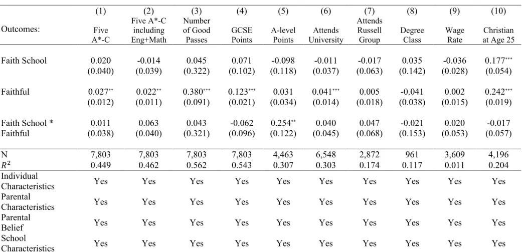
Regression results are presented below (with additional tables in the Appendix) and the pattern of controls is the same for each OLS table. The whole sample includes those of no religion, Protestants, and Catholics. Controls for the two Christian denominations are added in column (2). Individual characteristics are added in column (3). These are gender, ethnicity, month of birth, month of interview, and the individual’s academic performance at KS2. Parental/household characteristics (added in (4)) are the index of multiple depravation (IMD), whether the child is on free school meals (FSM), mother’s education, mother’s ethnicity, mother’s employment status, whether the child has a single mother, the number of dependent children in the household, and the region of residence. The mother’s employment and education are interacted with whether the father’s characteristics of the same variable are missing. Parental belief (in their religion and how important it is to them) is added in column (5). School characteristics (added in (6)) are whether the school has a particular specialism (for which they had been awarded additional funding), the percentage of students on FSM, whether the school is academically selective, whether the school has a “sixth form” (a senior high school for post-compulsory education), the size of the school and the size of the previous school attended, the percentages of students who have special needs, who are white, speak a first language that is not English, and whether the school has single sex intake.16 The column (6)
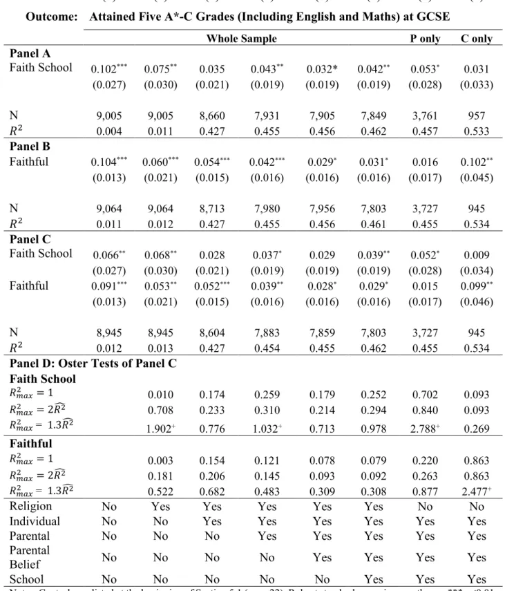
controls are used in the mediation analysis and in the outcome equation of the IPWRA later. Tables 3 and 4 report regression results for two GCSE outcomes; whether or not the individual attained 5 A*-C grades, including English and Maths, and the number of “good” passes that the individual achieved – i.e. how many grades were they awarded at C or above. Columns (1) to (6) show results for the whole sample whilst columns (7) and (8) show only the Protestant (P) and Catholic (C) subsamples. Each table, as will be the case in each of the OLS tables, presents four panels. The first (Panel A) shows the regression results, across numerous specifications, where faithfulness is not included - the only “treatment” is attendance at a faith school. The second (Panel B) is the opposite, faith school is not included - the only treatment is whether the individual is faithful. Panel C includes both treatments together. The reasoning behind presenting the results in such depth is to show the stability of coefficients upon the inclusion of both treatments of interest together. An obvious concern if only panel C was shown
25
would be that one treatment was sapping the significance associated with the other due to the obvious correlation between being more devout and wanting to attend a faith school. This concern is all the more valid considering the papers cited above that suggest a positive effect of faith school attendance on religiosity (e.g. Wadsworth and Walker 2017)). Panel D, to be explained later, presents the Oster (2019) test results.
Looking at Table 3 it appears that both faith school and faithfulness have impacts on the likelihood that an individual attains the benchmark of five A*-C grades (with the added condition that those grades include English and Maths) in a linear probability model. These are each significant; at the five and ten percent levels respectively. The magnitudes are not insubstantial, attending a faith school appears to increase the likelihood of attaining the benchmark by around four percentage points, and being faithful compared to unfaithful by three percentage points. Comparing the coefficients in Panel C to the corresponding coefficients in Panels A and B, it is easy to see that the inclusion of both treatments simultaneously does not seem to alter the coefficient magnitudes by any meaningful amount – indeed the difference is never different in a statistical sense.
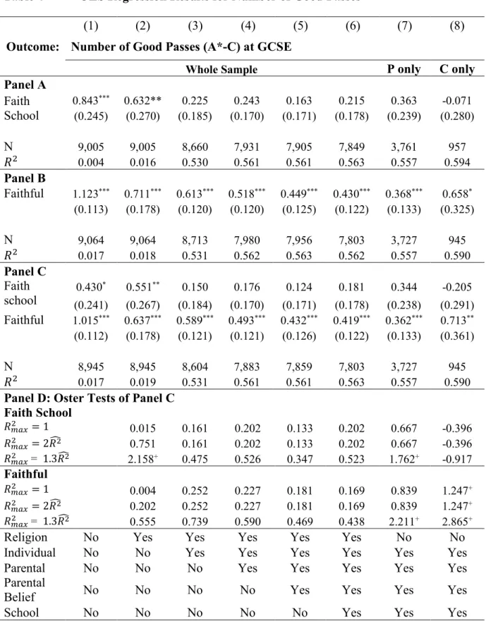
Turning to Table 4, where the outcome is number of good passes at GCSE, a number of points stand out. The first is that faith schooling does not appear to have an impact once exogenous individual characteristics (gender, ethnicity, month of birth, and prior attainment at primary school) are accounted for. The second is that faithfulness does – and it has a large impact at that. It is also always significant at the one percent level, except in the Catholic case where the significance is at the five percent level in Panel C. Taking column 6, which includes the whole sample and the full range of covariates, it appears that around 0.4 of an additional pass could be gained by being faithful compared to unfaithful. These numbers, as in Table 3, are remarkably stable when comparing the panels that include the two treatments separately with their simultaneous inclusion.17 This same pattern is repeated for the GCSE point score outcome – essentially the same outcome but more granular. This is given in the Appendix Table A6.18
17 As we are interested in faith school effects, we cannot include school fixed effects as the faith school coefficient is omitted
from regressions. When faithfulness alone is the treatment, however, we can and do include fixed effects (not shown) – the results are virtually unchanged from what is shown in this paper when the full range of controls is included.
18 Interestingly, the same pattern is also replicated by subject. Regression results (not shown) for highest English grade attained,
maths grade attained, and highest science grade attained show the same pattern as the number of good passes outcome. This suggests that faith schools, as well not being stronger overall, are not any stronger in particular subjects.
26
Table 3 OLS Results for Attained Five A*-C Grades (incl. English and Maths)
(1) (2) (3) (4) (5) (6) (7) (8)
Outcome: Attained Five A*-C Grades (Including English and Maths) at GCSE
Whole Sample P only C only
Panel A Faith School 0.102*** 0.075** 0.035 0.043** 0.032* 0.042** 0.053* 0.031 (0.027) (0.030) (0.021) (0.019) (0.019) (0.019) (0.028) (0.033) N 9,005 9,005 8,660 7,931 7,905 7,849 3,761 957 𝑅𝑅2 0.004 0.011 0.427 0.455 0.456 0.462 0.457 0.533 Panel B Faithful 0.104*** 0.060*** 0.054*** 0.042*** 0.029* 0.031* 0.016 0.102** (0.013) (0.021) (0.015) (0.016) (0.016) (0.016) (0.017) (0.045) N 9,064 9,064 8,713 7,980 7,956 7,803 3,727 945 𝑅𝑅2 0.011 0.012 0.427 0.455 0.456 0.461 0.455 0.534 Panel C Faith School 0.066** 0.068** 0.028 0.037* 0.029 0.039** 0.052* 0.009 (0.027) (0.030) (0.021) (0.019) (0.019) (0.019) (0.028) (0.034) Faithful 0.091*** 0.053** 0.052*** 0.039** 0.028* 0.029* 0.015 0.099** (0.013) (0.021) (0.015) (0.016) (0.016) (0.016) (0.017) (0.046) N 8,945 8,945 8,604 7,883 7,859 7,803 3,727 945 𝑅𝑅2 0.012 0.013 0.427 0.454 0.455 0.462 0.455 0.534
Panel D: Oster Tests of Panel C Faith School 𝑅𝑅𝑚𝑚𝑚𝑚𝑚𝑚2 = 1 0.010 0.174 0.259 0.179 0.252 0.702 0.093 𝑅𝑅𝑚𝑚𝑚𝑚𝑚𝑚2 = 2𝑅𝑅�2 0.708 0.233 0.310 0.214 0.294 0.840 0.093 𝑅𝑅𝑚𝑚𝑚𝑚𝑚𝑚2 = 1.3𝑅𝑅�2 1.902+ 0.776 1.032+ 0.713 0.978 2.788+ 0.269 Faithful 𝑅𝑅𝑚𝑚𝑚𝑚𝑚𝑚2 = 1 0.003 0.154 0.121 0.078 0.079 0.220 0.863 𝑅𝑅𝑚𝑚𝑚𝑚𝑚𝑚2 = 2𝑅𝑅�2 0.181 0.206 0.145 0.093 0.092 0.263 0.863 𝑅𝑅𝑚𝑚𝑚𝑚𝑚𝑚2 = 1.3𝑅𝑅�2 0.522 0.682 0.483 0.309 0.308 0.877 2.477+
Religion No Yes Yes Yes Yes Yes No No
Individual No No Yes Yes Yes Yes Yes Yes
Parental No No No Yes Yes Yes Yes Yes
Parental
Belief No No No No Yes Yes Yes Yes
School No No No No No Yes Yes Yes
Notes: Controls are listed at the beginning of Section 5.1 (page 22). Robust standard errors in parentheses; *** p<0.01, ** p<0.05, * p<0.1. + indicates passing of robustness threshold in the Oster (2017) test.