Neural Network Handoff Algorithm in a Joint Terrestrial-HAPS Cellular System

Neural Network Handoff Algorithm in a Joint

Terrestrial-HAPS Cellular System

Raungrong Suleesathira

Sunisa Kunarak

, Non-members

ABSTRACT

Handoff algorithm is used in wireless cellular sys-tems to decide when and to which base station (BS) to handoff in order that the services can be continued uninterrupted. In this paper, we propose a handoff algorithm based on the neural network in a joint sys-tem of terrestrial and high altitude platform station (HAPS) cellular systems. As a revolutionary wireless system, HAPS can supply services for uncovered area improving total capacity of service-limited area by a terrestrial BS. Radial-Basis function (RBF) network is used for making a handoff decision to the chosen neighbor BS. The neural inputs consist of the aver-aged signal strength received from the serving and nearby BSs, user directions estimated by the MUSIC algorithm on an antenna array, and traffic intensi-ties. Positioning a mobile station (MS) is obtained by apply the timing advance (TA) concept. Perfor-mance comparisons among the presented method and using the backpropagation (BP) neural network and the conventional Hysteresis method are given in forms of (1) handoff rate, blocking rate, dropping rate at the acceptable grade of service and (2) the difference be-tween the signal power radiated by the serving BS and the minimum required received signal power be-fore call dropping for both Hata model and Rayleigh fading.

Keywords: Handoff, Radial-basis function net-works, Backpropagation netnet-works, MUSIC, Timing advance, Rayleigh fading.

1. INTRODUCTION

In mobile communications, the continuity of com-munication without terminating an ongoing call or blocking new calls is very crucial to enhance high quality of cellular services. Handoff algorithm makes it possible to maintain link quality. In Hysteresis method [1], handoff occurs when the difference of sig-nal strength received from target and current BSs is higher than Hysteresis level. Because of fading ef-fect, the difference can be fluctuated for brief periods of time which results in unnecessary handoffs. Such CM1R38: Manuscript received on August 28, 2004 ; revised on June 25, 2005.

The authors are with the Department of Electronic and Telecommunication Engineering King Mongkut’s University of Technology Thonburi, Tungkru, Bangkok, 10140 Thailand. E-mail: [email protected]

back and forth handoff is known as the ping-pong effect. In addition to network resource waste, calls might be terminated if decision delay is long due to the high Hysteresis level.

Recently, neural networks have been utilized to im-prove handoff algorithms due to its ability to handle large data in fast processing. Adaptive parameters such as user speeds, received signal strengths for pat-tern classification provide a multiple of criteria hand-off algorithm [2]. Neural network is trained to pre-dict a user’s transfer probabilities which represent the user movements [3]. A technique to recognize signal patterns of a MS using probabilistic neural network is introduced in Rayleigh fading channel [4]. Using statistical pattern recognition of signal strength [5-6] can improve the efficiency of handoff algorithms.

In this paper, we present an effective handoff algo-rithm based on radial basis function (RBF) networks [7] in a joint terrestrial-HAPS cellular system [8]. Fig-ure 1 shows the conceptual model of the joint cellu-lar system. The inputs of neural network depend on signal strengths, mobile directions and traffic inten-sities, which are used to make a handoff decision to the chosen adjacent cell or HAPS. We use an antenna array with the MUSIC [9] (MUltiple SIgnal Classifi-cation) to estimate directions of arrival of MS signals. The signal strengths of mobiles are computed in the Hata model and Rayleigh fading [10]. HAPS cellu-lar system can be considered as a complementary to the terrestrial cellular system, to improve and expand the coverage services. As shown in Fig. 1, HAPS can supply services to the mobile having weak signal from the serving terrestrial BS influenced by shadowing, turning corner as well as being outside the terrestrial coverage. The timing advance (TA) concept [11-12] in GSM system and the power of mobile signal are used for checking if the mobile are in an obstacle area.

This paper is organized as follow. Section 2 re-views the Hysteresis method. Handoff decision based on RBF network is presented in section 3 and based on the backpropagation network is next presented in section 4. The MUSIC algorithm is explained in sec-tion 5. The concept of timing advance is in secsec-tion 6. The handoff algorithm and HAPS improving the call maintenance are presented in section 7. Channel propagations for both Hata and Rayleigh are mod-eled in section 8. Section 9 illustrates the simulation results followed by conclusions.

Fig.1: The conceptual joint system model.

2. HYSTERESIS METHOD

A traditional handoff algorithm which is known as the Hysteresis method uses relative signal strength as a main component in the handoff decision process. In Fig. 2, the mobile is moving from the serving BS to another BS. To have an ongoing call, we need to hand-off when the relative signal strength received from the target base rises above the Hysteresis margin dB. It corresponds to the distance at point C. For GSM sys-tem, handoff from one cell to another cell is decided when [1]

RSS AV G=_{RSS AV GT} −_{RSS AV GS} ≥_h where _{RSS AV G} is the difference between the averaged received signal strength from the tar-get cell (_{RSS AV GT}) and from the serving cell (_{RSS AV GS}). However, the smaller _his, the more frequent the unnecessary handoffs would happen. In this case, it might result in repeated handoffs between the two BSs caused by rapid fluctuations in the re-ceived signal. It is so-called the ping-pong effect. On the other hand, having the larger_hcan increase the decision delay that might cause call dropping. There is therefore a tradeoff between the number of unnec-essary handoffs and decision delay.

Thus, we propose an improved handoff algorithm based on RBF networks that consider mobile loca-tion, direcloca-tion, averaged signal power and cell traffic intensity. Namely, the input to the neural network is not only the received signal strengths, but it is also the direction of mobile moving to the target cell and

the traffic intensities of the neighbor cells. It makes the proposed approach capable of reducing the hand-off rates and blocking rates as well as dropping rates compared to the conventional Hysteresis method.

Fig.2: Location of a handoff decision in Hysteresis

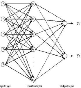
3. RADIAL-BASIS FUNCTION NETWORK

In this section, we apply radial-basis functions (RBF) to the neural network as depicted in Fig. 3 for making handoff decisions. The basic structure consists of three layers; input layer, hidden layer and output layer [7]. The number of nodes used in the hid-den layer is 20. This number was found after training the network and it made the errors converged. The Gaussian functions fully connect them to the five in-put nodesx= [_x1, . . . , x5]. The output node is a

lin-early weighted sum of the hidden unit outputs. The reason that we have two outputs is to reduce number of iterations of learning process. The outputs decide whether the system needs a handoff or not. If_y1and y2 are 00, no handoff will be performed. Ify1andy2

are 11, then the system will handoff the mobile to the chosen base station.

The network is trained by the following pro-cedure to find the weight vector,w_k1(n) =

[_wk(_n)_{, . . . , wk}20(n)], starting at the iterationn= 0.

1. Initialize the center value_µji(0) of the_ithinput node and the_jthhidden node.

2. Initialize the span value_σj(0) of the_jthhidden node.

3. Initialize the weight vectorw_k(0). Note that 1-3 are initialized using a uniform distribution between [0, 1] except_w11(0) =w21(0) = 1.

4. Calculate the output of the hidden layer:

zj=exp− xi−µij(n)2/2σj2(n) 5. Calculate the output:

yk =R Mj=_iwkj(n)zj

, k= 1_,2;_M = 20 where_R[•] is a round operation.

6. Calculate the error: _ek =_dk−_yk where _dk ∈

Fig.3: Radial-basis function network

7. Update the weight: _wkj(_n+ 1) = _wkj(_n) +

ηwekzj where ηw is the learning rate of weight. 8. Update the center momentum:

µij(n+ 1) =µij(n) +ηµ_σzj_j(xi−µji(n))ekwkj(n) where_ηµ is the learning rate of center.

9. Update the span:

σj(n+ 1) =σj(n)−2_ση_jσ(_nzj)lnzj

ekwkj(n) where_ησ is the learning rate of span.

10. Repeat steps 4-9 until the mean square error converges less than a small fixed number.

The inputs to the neural network are listed below. 1. _x1 is the direction of a user. Under an

assump-tion that the mobile travels in unchanged direcassump-tion, it can be estimated using the MUSIC algorithm which will be described in the next section.

2. _x2is the signal strength of mobile received from

the serving BS.

3. _x3is the signal strength of mobile received from

the target BS. The received signal strength (RSS) is leveled as:

low: −96_{< RSS} ≥ −87dBm and high: _{RSS >}−87 dBm.

4. _x4is the traffic intensity (TI) of the serving BS.

5. _x5 is the TI of the target BS. The TI is leveled as

low: _{T I <}0_.6591 Erlangs/Channel

medium: 0_.6591≥_{T I} ≥0_.76 Erlangs/ Channel high: _{T I >}0_.76 Erlangs/Channel

Note that, we use the GOS (Grade of Service) in the range 2-5% and the system has 20 channels to design the TI levels. From the Erlang B table [10], TI equals to 13.1816 when the GOS is 2% and equal to 15.2 for 5%. Thus, the traffics per channel are equal to 0.6591 and 0.76, respectively.

Fig.4: Mean square errors in the trained network

The proposed handoff decision by the neural net-work depends on both RSSs and TIs of the serving (S) and target (T) BSs. We consider four cases as ordered in Table 1 which are

1) Both the RSSs from the serving and target BSs are low.

2) The RSS from the serving BS is low while the RSS of the target BS is high.

3) Both the RSSs from the serving and target BSs are high.

4) The RSS from the serving BS is high while the RSS from the target BS is low.

In each case, there are different handoff decisions (HO: handoff or NOHO: no-handoff) regarding to the levels of traffic intensity.

Consider a particular case that the RSS from the serving cell is low and the RSS of target cell is high and their both intensities are high. In this severe sit-uation, the neural network decides definitely to hand-off. If the target cell chosen by using has no channels available, we will consider among the adjacent cells and HAPS. The cell that has the highest RSS will be the cell to where mobile is handoffed.

In our implementation, 5000 samples are used for training the network and 500 samples are used to test the network. For training, it is found that the errors converge to zero as shown in Fig. 4. Figure 5 illus-trates the good performance of the network for testing data.

4. BACKPROPAGATION NEURAL NET-WORKS

The backpropagation (BP) structure shown in Fig. 6 has the same number of nodes in each layer as Fig. 3. Letx_p= (_xp1, x_p2, x_p3, . . . , x_pN) be a network

in-put vector for _N input nodes of _pththe learning se-quence. In the_nthiteration,_vij(_n) is the weight ele-ment connecting the_ith input node and the_jth hid-den node which is connected to the_kth output node

Table 1: Handoff decision

by_wjk(_n). In the forward propagation, the input of the_jth hidden node is

nethpj = N i=1

vij(n)xpi

where_vij(0) = 1. The output of the_jthhidden nodes for_j= 1_{, . . . , M} can be obtained as

zpj =ϕ(nethpj)

where _ϕ(_x) = ₁₊1_e−x is the sigmoid function. Once the output of the hidden node _zpj is found, we can

Fig.5: Mean square errors in the tested network

compute the input of the output layer as

net0pk= M j=1

wkj(n)zpj

where _wkj(0) = 1. Note that the weight vectors are initialized uniformly distributed between [0, 1]. The output of the_kthoutput node is a function as

ypk=R[ϕ(net0pk)]

In backward propagation, the procedure is started from the output layer to the input layer to adjust the output and hidden weights given as follows:

δpk=ϕ(net0pk)(dk−ypk)

where _ϕ(_x) represents the differential. Next, up-date the weight elements between the hidden and the output layers

∆_wkj(_n+ 1) =_ηδpkzpi+_µ∆_wkj(_n)_.

where_η is the learning rate and_µis the momentum. It is used to update the weight in the next iteration by adding

wkj(n+ 1) =wkj(n) + ∆wkj(n+ 1).

Likewise, the weights connecting the hidden and in-put layers are updated by using the following equa-tions. δpj =ϕ(neth_pj) k δpkwkj(n+ 1) ∆_vji(_n+ 1) =_ηδpjxpj+_µ∆_vji(_n) vji(n+ 1) =vji(n) + ∆vji(n+ 1).

After updating_vji(_n+ 1) and_wkj(_n+ 1), the forward propagation is repeated until the errors converge.

10000 samples are used for training and 500 sam-ples are used for testing. The convergence of error is shown in Fig. 7. Figure 8 shows the mean square error resulting from testing the network.

Fig.6: Back-propagation neural network.

Fig.7: Mean square errors in the trained network

5. THE MUSIC ALGORITHM

Consider the received signals impinging on_L uni-form linear array antennas which consist of the _M source signals corrupted by noise in the form of [9]:

X(t) = M m=1 a(_θm)s_m(t) +_η(t) =A(Θ)s(t) +_η(t) whereA(Θ) = [a(_θ1)_{, . . . ,}a(_θM)] is an_L×_Msteering matrix whose column is a steering vector a(_θm) of the signal_sm(_t) having an unknown angle of arrival

θm. Θ = [θ1, . . . , θM] is an angle of arrival (AOA) vector of the_M source signal vector denoted ass(t) = [s₁(t)_{, . . . ,}s_M(t)]T with an assumption that_{M < L}. The steering vector can be written as:

a(_θm) = [1e−j2πdλsinθm_{. . .e}−j(L−1)2πdλsinθm_]T

where_d/λis the ratio of inter-element space of array to the signal wavelength. _η(t) = [_η1(t)_{, . . . , ηL}(t)]T

Fig.8: Mean square errors in the tested network

is a noise vector which is temporally and spatially white correlated.

The correlation matrixR of the array signal out-put can be written as

R=E[x(t)xH(t)]_.

An expression ofRin terms of eigenvalues and their corresponding eigenvectors is given as

R=UΛUH

where U = [u_{1, . . . ,}u_L]_L×L is a unitary matrix and Λ is a diagonal matrix of real eigenvalues _λi(_λ1 ≥

λ2≥. . .≥λ_L>0) corresponding to the eigenvector ui. Then, we decompose the correlation matrix R into a signal subspace: S= [u_{1, . . . ,}u_M] and a noise subspace: N= [u_M+1, . . . ,uL]. Thus, the matrixR

can be rewritten as a sum of the two subspaces:

R=SΛ_sSH+NΛ_nNH_.

As a result of orthogonality of the steering vectors to the noise subspace, the MUSIC algorithm estimates the AOA vector of the signals by finding_M peaks of

PMUSIC(θ) =|aH(θ)N|−2.

In practice, we cannot find the correlation matrixR, thus we use the sample-average estimate for_N snap-shots as ˆ R= 1 N N−1 t=0 x(t)xH(t)_.

Figure 9 shows an AOA estimate of the ten source signals corresponding to the ten peaks of MUSIC. The FSK signal is used and defined as [13]

s(_t) =

2_Es

T cos[ωct+θ(t)]

where_ωcis the carrier frequency,_θ(_t) the phase of the signal,_Es is the symbol energy and_T is the symbol

period. In simulation, we assign_T equal to 0.02 secs,

ω1 and _ω2 are equal to 100 and 200 Hz,_Es = 1 dB and_θ(_t) is generated using the uniform distribution in the range of 0−2_π. The number of antennas is used 30.

Fig.9: AOA estimates at4◦,63◦,107◦,137◦,179◦,

222◦,256◦,280◦,328◦,352◦.

6. TIMING ADVANCE

In the proposed handoff method, we need to know the mobile locations (_d) to check if the mobiles are in an obstacle position or in the 3-cell junction. Posi-tioning a mobile station is divided into two categories: network-based and handset-based positioning. We use one of handset-based technique called the timing advance (TA) [11-12] to determine where the mobile is.

TA is a measurement of the time required for the signal to travel from the MS to the BS. The concept of TA is used in order that the time-frames from each MS arrive at the correct time slot when received by the serving BS. By checking the position of the train-ing sequence transmitted from the MS on the uplink, the BS can calculate the TA value and send it back to the MS in the downlink. Then, it enables the mobiles to know when to send the frame so that the signals arrive at the BS in synchronism. For example, the value of TA in GSM system is an integer in a range of 0-63 according to 0 to 233 _µs. It defines 0 is to be no TA and 63 to be the maximum TA. Each TA number corresponds to different 550 m. radial dis-tance. It is reported to the MS every 480 ms during the connection.

In this paper, the TA is set in the range of 0 to 7 according to 0 to 7_µs. These values are coded by 3 bits. One bit of the TA represents a time difference of (7_µs)/7= 1_µsof the signal BS-MS-BS. The distance per bit of TA is_db= (3×108×1_µs)_/2 = 150 m/TA. The MS-BS distance is a function of the integer TA as

d(_{T A}) =_{T A}×_db

where _{T A} =_R[_ν∆_t/150] depending on the velocity of mobile_ν and a time interval of measurement ∆_t.

7. NEURAL NETWORK HANDOFF ALGO-RITHM

Figure 10 is a flow chart illustrating the proposed handoff algorithm. The capacity of the system is more efficient with the goodness of HAPS. First, we check if the mobile is staying in the obstacle position or even at the corners of 3-cell junction by monitor-ing if the mobile distance is_{d <}800 or_d≥1000 and if the RSS is less than the threshold. The threshold of the received signal strength (RSS drop) is at -82 dBm before call is dropped. If the mobile has the sig-nal strength received from the serving BS less than -82 dBm, a handoff from the serving terrestrial BS to HAPS-BS is necessary to improve the call quality. If 800 ≤ _d ≤ 1000, we measure the signal strength of the mobile received from the current and adjacent cells every 0.5 sec. In order to decrease variation of the signals, an average of 10 data is calculated. After obtaining the averages of signal strength of current and neighbor cells of_x1, we can determine which cells

are most likely to be the target base stations (BST(i)) by checking that the mobile receives the signal power from which base stations radiate greater than -96 dBm (RSS low TH). Included the knowledge of the mobile directions obtained by the MUSIC algorithm and traffic intensities of the chosen BSs, the trained neural network then makes a decision if the mobile needs a handoff or not. In the case of deciding to handoff, the algorithm will assign either case (1) to which base station the mobile will be handoffed or (2) request a channel from HAPS. Note that HAPS gives higher priority to handoff-calls than new-calls such that probabilities of blocking calls are low.

8. MOBILE RADIO PROPAGATION MODEL 8. 1 Hata Model

The path loss in Hata model is expressed as [10]

PL= 69.55 + 26.16logfc−13.82loghb−a(h) + (44.9− 6_.55log_hm)log_d

where _a(_h) = 3_.26(log11_.75_hm)2₋₄

.97 for a carrier frequency_fc≥300 MHz,_hb is the height of antenna at base station (m) _hm is the height of antenna at mobile (m), _d is the distance between BS and MS (km). Accordingly, the strength of signal at a mobile is

RSS=_P0−P_L

where_P0denotes the power radiated from the BS.

8. 2 Shadow-Rayleigh Fading

In mobile radio channels, the Rayleigh distribution [4,10] is commonly used to model a flat fading chan-nel. This small-scale fading describes the statistical time varying nature of the received envelope. It is

Fig.10: Handoff algorithm using neural network.

well known that the sum of signals with the random amplitudes and phases by no direct path between a MS and a BS obeys a Rayleigh distribution. The en-velope of the received signal strength_rk at a MS-BS distance_dhas a probability density function given by

p(_rk) = rk pkexp − r2k 2_pk , 0≤_rk ≤ ∞ where _pk is the time-average power of the received signal strength before envelope detection. The mean value of the Rayleigh distribution is _E[_rk] = _πpk

2 . The received signal power with an arbitrary

transmitter-receiver separation distance is modeled as using the path loss exponent from 2 to 6.

The shadow fading process is a Gaussian dis-tributed random process measured in decibels (dB). Under lognormal shadow fading, the autocorrelation is given as

RL(d) =σL2exp −|_d0d|

where _σL2 and _d0 are the variance and correlation

length of shadow fading, respectively. Accordingly, the power spectral density_SL(_v) can be found as

SL(v) = 2d0σ

2

L 1 + (2_πvd0)2

where _v is a spatial frequency. For a total traveled distance_D, the shadow fading process can be written as L(_d) = J j=−J 2 BDSL j D cos 2πjd D +φj where B= 1 σ2 LD J j=−J SL j D , J =_Dvm.

Let_vmbe the maximum spatial frequency and_φj be an identically independent uniform random process in range of 0−2_π. The discrete process_Lk is obtained by sampling the process at_d=_dk.

The received signal strength (RSS in dB) in the presence of Rayleigh fading is in the form of

sk= 20log10rk

where _rk is a Rayleigh distribution random variable with parameter _pk = (1_/2)10mk/10_{. The power can}

be calculated in dB as

mk =P0−10nlog10d_k+L_k.

The mean and variance of are given as ¯ sk = 10log10(2pk)− 10_γ ln10 = _mk− 10γ ln10 σ2sk = 50_π2 3ln210 where_γ≈0_.577216 is Euler’s Gamma.

9. SIMULATION RESULTS

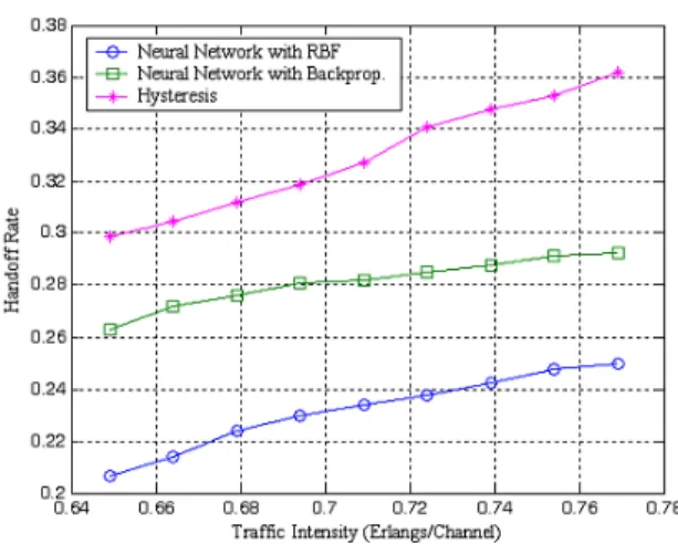
The performance of the handoff algorithm using the RBF and BP neural networks is illustrated in comparison to the Hysteresis method. Simulations are done for the system pictorially shown in Fig. 1. 200 trials are run at a fixed traffic intensity and at a fixed mean arrival time of the serving BS. The car-rier frequency is_fc = 1800 MHz. The antenna height is 60 m at BS and 1.5 m. at MS. The parameters of cell environment and the statistical parameters of mo-bile are listed in Table 2-3. To evaluate the proposed method and Hysteresis rule, the handoff rate (H/_Th), blocking rate (B/T) and dropping rate (D/_Th) are computed at the serving BS (cell no. 1). H represents the number of successful handoffed calls; Th repre-sents the total number of calls decided to handoff; B represents the number of blocked calls; _Th repre-sents the total number of new calls; D reprerepre-sents the number of dropped calls. There are two cases in each channel model. First, we vary the traffic intensities in the range of 0.65-0.77 Erlang/channel for acceptable GOS 2-5% of the cell No. 1 at the mean arrival time equal to 1 min. In the other case, we vary the mean arrival time from 3-5 mins.

In Hata path loss propagation, Figs. 11-17 show that handoff algorithm using the RBF network out-performs that using BP network and Hysteresis. Handoff rate, blocking rate and dropping rate result-ing from usresult-ing RBF network are lowest in any case

of traffic intensities and mean arrival times as plotted in Figs. 11-16. Since we consider the signal strength, position, direction and traffic intensity, the unnec-essary handoffs is reduced as seen in Figs. 11 and 14. The resulting blocking rates in Figs. 12 and 15 have also low probabilities. As a result of the reduced unnecessary handoffs and HAPS, there are more available channels for new calls to access the sys-tem. We also achieved the reduction of dropping rates as shown in Figs. 13 and 16 because once the handoff rate decreases, chance of dropping is also less. Fig. 17 depicts the number of handoffs occurring at the difference between the signal power of mobile receiv-ing from the current BS and the minimum received signal strength (-96 dBm) that the call will dropped. In fact, the less power difference, the more number of handoffs. Using the proposed algorithm, low number of handoffs at low power difference is achieved. For Hysteresis rule, the power difference should higher than 6 dB to avoid call-dropping.

In shadow-Rayleigh fading, we assign the Rayleigh fading parameters in Table 3. Similarly, the results obtained from the proposed method using the RBF network are the best among using BP network and using Hysteresis as shown in Figs.18-24.

10. CONCLUSION

We propose an effective handoff algorithm based on RBF network in high altitude platform station cel-lular systems. HAPS system can provide services to the users staying at the corner of cells or at covered area influenced by shadowing. Besides the averaged received signal strength, user position and direction and traffic intensity are inputs of the neural networks. We use the RBF and BP to construct the networks. The MUSIC technique in the antenna array provides us an estimate of user direction. Timing advance used in the GSM system is applied to this system for mo-bile positioning. Consequently, handoff rate, blocking rate and dropping rate decrease compared with the traditional Hysteresis algorithm. The simulations are performed in large scale channel propagation which is the model of Hata path loss, and small scale channel propagation in the process of Rayleigh fading. Be-sides the lower rates, we achieve low difference be-tween the mobile signal power from the target BS and the minimum required power before dropping calls at a few needed numbers of handoffs.

References

[1] S. Ulukus and G. P. Pollini, “Handover Delay in Cellular Wireless Systems,” IEEE International Conference on Communications, pp. 1370-1374, Jun. 1998.

[2] N. D. Tripathi, J. H. Reed and H. F. Van Landing-ham,“Pattern Classification Based Handoff Using Fuzzy Logic and Neural Nets,” IEEE

Interna-tional Conference on Communications, Vol. 3, pp. 1733-1737, Jun. 1998.

[3] W. W. H. Yu and H. Changhua, “Resource Reser-vation in Wireless Networks based on Pattern Recognition,” International Joint Conference on Neural Networks., Vol. 3, pp. 2264-2269, Jul. 2001.

[4] R. Narasimhan and D. C. Cox, “A Handoff Algo-rithm for Wireless Systems Using Pattern Recog-nition,” 9th IEEE International Symposium on Personal Indoor and Mobile Radio Communica-tions, Vol.

[5] K. D. Wong and D. C. Cox, “A Pattern Recogni-tion System for Handoff Algorithms,”IEEE Jour-nal on Selected Areas in Communications, Vol. 18, No. 7 pp. 1301-1312, Jul. 2000.

[6] K. D. Wong and D. C. Cox, “Two-State Pattern-Recognition Handoffs for Corner-Turning Situa-tions,” IEEE Transaction on Vehicular Technol-ogy, Vol. 50, No. 2, pp. 354-363, Mar. 2001. [7] S. Haykin, Neural Networks: A Comprehensive

Foundation, Prentice Hall, 1999.

[8] S. Masumura and M. Nakagawa, “Joint System of Terrestrial and High Altitude Platform Station (HAPS) Cellular for W-CDMA Mobile Communi-cations,” IEICE Transaction on Communication, Vol. E85-B, No. 10, pp. 2051-2058, Oct. 2002. [9] R. Suleesathira, “Close Direction of Arrival

Es-timation for Multiple Narrowband Sources,” 7th

IEEE International Symposium on Signal Pro-cessing and Its Applications, Vol. 2, pp. 403-406, Jul. 2003.

[10] T. S. Rappaport, Wireless Communications: Principles and Practice, Prentice Hall, 2002. [11] G. P. Yost and S. Panchapakesan, “Improvement

in Estimation of Time of Arrival (TOA) from Timing Advance (TA),”IEEE International Con-ference on Universal Personal Communications, Vol. 2, pp. 1367-1372, Oct. 1998.

[12] http://www.willassen.no/msl/node6.html [13] B. Sklar,Digital Communications Fundamentals

and Application, Prentice Hall, 2001.

Raungrong Suleesathirareceived the B.S. degree in 1994 from Kasetsart Uni-versity, Bangkok, Thailand and the M.S. and Ph.D. degrees from University of Pittsburgh, PA, in 1996 and 2001, re-spectively, all in Electrical Engineering. Since 2001, she has been on the fac-ulty of the Department of Electronics and Telecommunication Engineering at King Mongkut’s University of Technol-ogy Thonburi, Thailand where she is now an Assistant Professor. Her current research interests are in the areas of smart antennas and wireless communications.

Sunisa Kunarak received the B.S. degree in Electronics and Telecommu-nication Engineering and M.S. degree in Electrical Engineering from King Mongkut’s University of Technology Thonburi, Thailand in 2002 and 2004, respectively. Currently, she works as a communication engineer for process-ing mobile signals in subways at Bombar Dier Transportation (Signal) Thailand.

Table 2: Cell Structure Parameters

Parameters value

cell radius 1000 m

number of channels per cell 20 channels number of channels in HAPS 20 channels low threshold of received signal -96 dB

strength (RSS low T H)

received signal strength for call -82 dB dropping (RSS drop)

Power Transmittedp0 40 dBm Hysteresis level (h) 6 dB

Table 3: Mobile Parameters

variable distribution interval initial position in the Uniform [-10,10]

horizontal (m)

initial position in the Uniform [-8,8] vertical (m)

number of users in Uniform [100,400] each cell

mean arrival time of Poisson 1 min new call

direction of mobile Uniform [0,2π] average time per call Exponential 120 sec average mobile speed Normal N(60,10)

km/hr

Table 4: Rayleigh Fading Parameters

Parameters value

Minimum Base Station Separation 1600 m Exponent of Distance Dependence (n) 4 Standard Deviation of Shadow FadingσL 8 dB

Correlation Length of Shadow Fadingd0 20 m Number of terms for Shadow Fading Process 321

Maximum Spatial Frequency 0.1

Fig.11: Handoff rate versus traffic intensity in Hata

Fig.12: Blocking rate versus traffic intensity in Hata

Fig.13: Dropping rate versus traffic intensity in Hata

Fig.14: Handoff rate versus mean arrival time in Hata

Fig.15: Blocking rate versus mean arrival time in Hata

Fig.16: Dropping rate versus mean arrival time in Hata

Fig.17: Signal difference versus number of handoffs in Hata

Fig.18: Handoff rate versus traffic intensity in Rayleigh

Fig.19: Blocking rate versus traffic intensity in Rayleigh

Fig.20: Dropping rate versus traffic intensity in Rayleigh

Fig.21: Handoff rate versus mean arrival time in Rayleigh

Fig.22: Blocking rate versus mean arrival time in Rayleigh

Fig.23: Dropping rate versus mean arrival time in Rayleigh

Fig.24: Signal difference versus number of handoffs in Rayleigh