Web Effort Estimation:
Function Points Analysis vs. COSMIC
Sergio Di Martinoc, Filomena Ferruccia, Carmine Gravinoa,∗, Federica Sarrob
aDepartment of Computer Science, University of Salerno bCREST, Department of Computer Science, University College London
c Dipartimento di Ingegneria Elettrica e delle Tecnologie dell’Informazione, University of Napoli “Federico II”
Abstract
Context: Software development effort estimation is a crucial manage-ment task that critically depends on the adopted size measure. Several Func-tional Size Measurement (FSM) methods have been proposed. COSMIC is considered a 2nd generation FSM method, to differentiate it from Function Point Analysis (FPA) and its variants, considered as 1st generation ones. In the context of Web applications, few investigations have been performed to compare the effectiveness of the two generations. Software companies could benefit from this analysis to evaluate if it is worth to migrate from a 1st generation method to a 2nd one.
Objective: The main goal of the paper is to empirically investigate if COS-MIC is more effective than FPA for Web effort estimation. Since software companies using FPA cannot build an estimation model based on COSMIC as long as they do not have enough COSMIC data, the second goal of the paper is to investigate if conversion equations can be exploited to support the migration from FPA to COSMIC.
Method: Two empirical studies have been carried out by employing an industrial data set. The first one compared the effort prediction accuracy obtained with Function Points (FPs) and COSMIC, using two estimation
∗Corresponding author
Email addresses: [email protected](Sergio Di Martino),
[email protected](Filomena Ferrucci),[email protected](Carmine Gravino),
techniques (Simple Linear Regression and Case-Based Reasoning). The sec-ond study assessed the effectiveness of a two-step strategy that first exploits a conversion equation to transform historical FPs data into COSMIC, and then builds a new prediction model based on those estimated COSMIC sizes. Results: The first study revealed that, on our data set, COSMIC was sig-nificantly more accurate than FPs in estimating the development effort. The second study revealed that the effectiveness of the analyzed two-step process critically depends on the employed conversion equation.
Conclusion: For Web effort estimation COSMIC can be significantly more effective than FPA. Nevertheless, additional research must be conducted to identify suitable conversion equations so that the two-step strategy can be effectively employed for a smooth migration from FPA to COSMIC.
Keywords: Web effort estimation; Functional Size measures; COSMIC; IFPUG Function Point Analysis
1. Introduction
A crucial task for software project management is to accurately estimate the effort required to develop an application, since this estimate is usually a key factor for making a bid, planning the development activities, allocating resources adequately, and so on. Indeed, development effort, meant as the work carried out by software practitioners, is the dominant project cost, being also the most difficult to estimate and control. Significant over- or under-estimates can be very expensive and deleterious for the competitiveness of a software company [1].
FSM methods are meant to measure the software size by quantifying the ”functionality” provided to the users. In particular, the Function Point Anal-ysis (FPA) was the first FSM method, defined in 1979 [2]. Since then, several variants have been proposed (e.g., MarkII and NESMA) with the aim of im-proving the size measurement or extending the applicability domains [3]. As a consequence, FSM methods are nowadays widely applied in the industrial field for sizing software systems and then using the obtained functional size as independent variable in estimation models. It is worth noting that all the above methods fall in the 1st generation of FSM methods, distinguishing them from COSMIC, which is considered a 2nd generation FSM method, due to several specific characteristics. In particular, COSMIC was the first FSM approach conceived to comply to the standard ISO/IEC14143/1 [4]. It is
based on fundamental principles of software engineering and measurement theory, and it was developed to be suitable for a broader range of application domains [5].
In the context of Web applications, few investigations have been per-formed to analyze and assess the use of FPA (e.g., [6][7][8]). A few studies have also been carried out on the use of COSMIC for sizing Web applications and estimating development effort [9][10][11][12][13]. However, no study com-pared the effectiveness of using COSMIC with respect to the use of FPA for Web effort estimation. Moreover, only few studies were based on industrial experiences, also due to the lack of suitable data sets including information about both COSMIC and FPA sizes, and effort data. Thus, there is the need for more empirical studies in this context that can support software compa-nies in the choice of one of these measurement methods. A possible empirical evidence that COSMIC is more effective than FPA for effort estimation could motivate those software companies that usually employ FPA to migrate to COSMIC. It is evident that the migration from the 1st generation measure-ment methods to the 2nd generation requires some additional costs. Indeed, not only it is necessary to acquire new expertise within the company, but there is also the need to compute again the size of the applications measured in the past with FPA, in order to use them to build new effort estimation models based on COSMIC [14][15] or for other purposes (e.g., productivity benchmarking).
These issues motivated our investigation. Thus, the main aim of this work is to assess whether COSMIC is more effective than FPA for the effort estimation of Web applications. To this end, we investigated the following research question:
RQ1a Is the COSMIC measure significantly better than FPs for estimat-ing Web application development effort by usestimat-ing Simple Linear Regression and Case Based Reasoning?
In the case we have indications that size in terms of COSMIC is more informative than the size in terms of FPs, it would be interesting to highlight which characteristics contribute more in such information [16]. Since for each application we have data about the Base Functional Components (BFCs) that give cumulatively the COSMIC size and FP sizes, we employed them to investigate which BFCs are more informative for predicting the effort. To this end, we investigated the following research question:
RQ1b Which COSMIC and FP BFCs are significant in estimating Web application development effort?
To answer RQ1a and RQ1b we performed an empirical study using data from 25 industrial Web applications. In particular, for RQ1a we employed two widely and successfully used techniques [17] for building effort estima-tion models, namely Simple Linear Regression (SLR), that is a model-based approach, and Case-Based Reasoning (CBR), that is a Machine Learning-based solution, for predicting the development effort1. On the other hand, to answerRQ1b, we verified the correlation between each BFC and the effort and we have analyzed the distribution of the BFCs with respect to the final size.
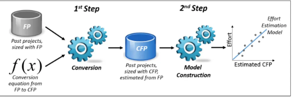
A positive answer to the first research question might motivate software companies to migrate from FPA to COSMIC for sizing new Web applications, but also raises the question on how to manage such a transition. Indeed, a company would be interested in how to start using COSMIC for effort esti-mation having only an internal database of past project measured with FPA, thus without any suitable estimation model for the new measure. The sim-plest strategy to estimate the effort of new applications, until there is not enough historical data based on COSMIC, is to remeasure the past projects with this method, but this requires a lot of time and effort and in soma cases it cannot be possible due to the lack of appropriate information. Another solution could be to exploit a (linear or non-linear) conversion equation pro-posed in the literature to obtain COSMIC sizes from the old FPs ones [14]. This allows the company to exploit its historical FPs data using a two-step estimation process (2SEP from here on) for building effort estimation models as shown in Figure 1. In more details, the first step consists of applying a conversion equation to each project in the historical data set, to get an es-timated COSMIC size starting from the FP one. This gives to the software company a new historical data set based on the estimated COSMIC. In the second step, it is possible to exploit this data set and SLR (or another esti-mation technique) to build a COSMIC based effort estiesti-mation model. This model can be used to predict the effort of the new applications, now sized
1Notice that we did not take into account other estimation methods, e.g., Support
Vector Regression [18] [19], Search-based approaches [20], and Web-COBRA [10], or com-bination of techniques, e.g., [21], since our focus was to compare FSM methods rather than specific techniques.
with COSMIC.
We are aware of the possibility that effort estimations based on estimated sizes can be less accurate than the ones based on measured sizes. A company would be interested in using 2SEP for a smooth migration if the obtained effort predictions have an accuracy at least not significantly worse than that obtained still using FPA. So, to analyze the effectiveness of 2SEP we inves-tigated the following research question:
RQ2a Is the Web effort estimation accuracy obtained employing 2SEP, with (linear and non-linear) external conversion equations, not significantly worse than the accuracy achieved by exploiting FPs in models built with SLR?
It is worth noting that another strategy for a software company could be to remeasure a sample of projects with COSMIC and use that subset to build an internal conversion equation that can be exploited in the first step of 2SEP to get an estimated COSMIC size for all the other projects of the historical data set. Nevertheless, this approach requires the extra effort to remeasure in terms of COSMIC at least a sample of projects. In the present paper we investigated also the effectiveness of 2SEP using conversion equations built on a sample of the 25 projects by analyzing how good was effort estimation using such company-specific equations. To this end, we investigated the following research question:
RQ2b Is the Web effort estimation accuracy obtained employing 2SEP, with (linear and non-linear) internal conversion equations, not significantly worse than the accuracy achieved by exploiting FPs in models built with SLR?
To answer RQ2a and RQ2b we performed a second empirical study em-ploying the same data set of 25 Web applications used in the first one, some external conversion equations and the internal conversion equations built considering a small sample of Web applications. To the best of our knowl-edge, the previous studies (e.g., [14] [22] [23]) investigating the conversion from FPs to COSMIC sizes focused only on showing that it is possible to build conversion equations, while the present study is the first that assesses the effectiveness of the sizes obtained using some conversion equations for effort estimation purposes.
The remainder of the paper is organized as follows. In Section 2 we briefly describe the FSM methods employed in our study, namely FPA and
Figure 1: The two-step process for building effort estimation models (2SEP).
COSMIC, and then we present related work on the use of FPA and COSMIC for Web effort estimation. In Sections 3 and 4 we present the two performed empirical studies. Threats to validity of both empirical studies are discussed in Section 5, while Section 6 concludes the paper giving some final remarks.
2. Background
In the following, we provide a brief history of FSM methods and recall the main notions of FPA and COSMIC.
2.1. A brief history of FSM methods
Software size measures can be grouped in two main families: the Func-tional and Dimensional ones. A Functional Size Measure is defined as “a size of software derived by quantifying the Functional User Requirements (FURs)” [4]. Thus, FSMs are particularly suitable to be applied in the early phases of the development lifecycle, when only FURs are available, being the typical choice for tasks such as estimating a project development effort. Moreover, they are independent from the adopted technologies, allowing com-parisons among projects developed with different platforms, solutions, and so on. Dimensional sizes basically count some structural properties of a software artifact, such as LOCs, number of Web pages, and so on. They can be ap-plied only after the artifact has been developed, they are strongly dependent on the adopted technological solutions, and often a standard counting pro-cedure is missing [24, 25]. The first FSM method proposed in the literature was the FPA, introduced by Albrecht in 1979 [2] as a measure (the Function Points) to overcome the limitations of LOCs, by quantifying the ”‘function-ality”’ provided by a software, from the end-user point of view. Indeed, FPA
can be seen as a structured method to perform a functional decomposition of the system. In this way, its size can be considered as the (weighted) sum of unitary elements (its FURs), that can be measured more easily than the whole system. FPA has evolved in many different ways. The original formu-lation was extended by Albrecht and Gaffney [26]. Then, since 1986 FPA is managed by the International Function Point Users Group (IFPUG) [27] and it is named IFPUG FPA (IFPUG, for short), which has been standardized by ISO as ISO/IEC 20926:2009. Nevertheless, since FPA was designed from the experience gained by Albrecht on the development of Management Infor-mation Systems, the applicability of this method to other software domains has been highly debated (e.g., [28, 29]). As a consequence, many variants of FPA were defined for specific domains, such as MkII Function Point for data-rich business applications, or Full Function Point (FFP) method for embedded and control systems [3]. Since these methods are all based on the original formulation by Albrecht, they are also known as 1st generation FSM methods.
In the middle of the 90’s, some researchers highlighted important issues in the foundations of FPA against the measurement theory. Indeed, in many steps of the FPA process an improper use of different types of scales was highlighted. Moreover, how the ”‘weights”’ were defined and used in the method has been object of discussion in the literature (e.g., [30, 31]).
To overcome these issues, and also to define a broader measurement framework able to tackle new IT challenges, at the end of the 90’s a group of experienced software measurers formed the Common Software Measurement International Consortium (COSMIC), whose result was the COSMIC-FFP method, which is considered the first “2nd generation FSM method”. To highlight this concept, the first version of the method was the 2.0. Many im-portant refinements were introduced in 2007 in the version 3.0, named simply COSMIC, and standardized as ISO/IEC 19761:2011. The current version of COSMIC is 4.0.1, introduced in April 2015.
In the following we describe the main concepts underlying the IFPUG and the COSMIC methods. Among the 1st generation methods, we analyze IFPUG since it is the most widely used by software practitioners.
2.2. The IFPUG method
IFPUG sizes an application starting from its FURs (or by other software artifacts that can be abstracted in terms of FURs).
In particular, to identify the set of “features” provided by the software, each FUR is functionally decomposed into Base Functional Components (BFC), and each BFC is categorized into one of five Data or Transactional BFC Types. The Data functions can be defined as follows:
• Internal Logical Files (ILF) are logical, persistent entities maintained by the application to store information of interest.
• External Interface Files (EIF) are logical, persistent entities that are referenced by the application, but are maintained by another software application.
The Transactional ones are defined as follows:
• External Inputs (EI) are logical, elementary business processes that cross into the application boundary to maintain the data on an Internal Logical File.
• External Outputs (EO) are logical, elementary business processes that result in data leaving the application boundary to meet a user require-ments (e.g., reports, screens).
• External Inquires (EQ) are logical, elementary business processes that consist of a data trigger followed by a retrieval of data that leaves the application boundary (e.g., browsing of data).
Once the BFCs have been identified, the “complexity” of each BFC is as-sessed. This step depends on the kind of function type and requires the identification of further attributes (such as the number of data fields to be processed). Once derived this information, a table provided in the IFPUG method [27] specifies the complexity of each function, in terms of Unadjusted Function Points (UFP).
The sum of all these UFPs gives the functional size of the application. Subsequently, a Value Adjustment Factor (VAF) can be computed to take into account some non-functional requirements, such as Performances, Reusabil-ity, and so on. The final size of the application in terms of Function Points is given by F P =U F P ·V AF.
For more details about the application of the IFPUG method, readers may refer to the counting manual [27].
2.3. The COSMIC method
The basic idea underlying the COSMIC method is that, for many types of software, most of the development efforts are devoted to handle data move-ments from/to persistent storage and users. Thus, the number of these data movements can provide a meaningful sight of the system size [5]. As a con-sequence, the measurement process consists of three phases:
1. The Measurement Strategy phase is meant to define the purpose of the measurement, the scope (i.e. the set of FURs to be included in the measurement), the functional users of each piece of software (i.e. the senders and intended recipients of data to/from the software to be measured), and the level of granularity of the available artifacts. 2. The Mapping Phase is a crucial process to express each FUR in the
form required by the COSMIC Generic Software Model. This model, necessary to identify the key elements of a FUR to be measured , as-sumes that (I) each FUR can be mapped into a unique functional process, meant as a cohesive and independently executable set of data movements, (II) each functional process consists of sub-processes, and (III) each sub-process may be either a data movement or a data ma-nipulation. To measure these data movements, three other concepts have to be identified. A Triggering Event is an action of a functional user of the piece of software triggering one or more functional processes. A Data Group is a distinct, non-empty and non-ordered set of data at-tributes, where each attribute describes a complementary aspect of the same object of interest. A Data Attribute is the smallest piece of in-formation, within an identified data group, carrying a meaning from the perspective of the interested FUR. As depicted in Figure 2, data movements are defined as follows:
• An Entry (E) moves a data group from a functional user across the boundary into the functional process where it is required. • An Exit (X) moves a data group from a functional process across
the boundary to the functional user that requires it.
• A Read (R) moves a data group from persistent storage within each of the functional process that requires it.
• A Write (W) moves a data group lying inside a functional process to persistent storage.
Figure 2: The four types of Data Movements, and their relationship with a Functional Process [5]
3. TheMeasurement Phase, where the data movements of each functional process have to be identified and counted. Each of them is counted as 1 COSMIC Function Point (CFP) that is the COSMIC measurement unit. Thus, the size of an application within a defined scope is obtained by summing the sizes of all the functional processes within the scope. For more details about the COSMIC method, readers are referred to the COSMIC Measurement Manual [5].
2.4. Related work
In the literature there is a number of studies on the assessment of FPA and COSMIC methods for effort estimation. However, very few of them investigate their effectiveness for Web applications. It is worth to mention that besides Function Points and COSMIC, other size measures (e.g., di-mensional measures like number of Web pages, media elements, client and server side scripts, etc.) have been proposed in the literature to be employed specifically for Web application development effort in combination with sev-eral estimation techniques [32] [33] [34] [35] [36] [37]. However, since our focus is on the use of FPA and COSMIC measurement methods, in the fol-lowing we first report on investigations exploiting FPA (Section 2.4.1) and then those employing COSMIC (Section 2.4.2), also considering their exten-sions/adaptions.
We will discuss the main studies proposing conversion models from FPs into COSMIC in Section 4.1. It is worth noting that the analysis about the effectiveness of internal vs external conversion equations is related to the
studies investigating the use of cross- vs within-company data sets for effort estimation. This topic has been widely analyzed in the last years producing different results (see e.g., [38]).
2.4.1. Using FPA and its extensions for Web effort estimation
FPA was employed by Ruheet al. [39] to size 12 Web applications, such as B2B, intranet or financial, developed between 1998 and 2002. The aim was to compare the effort estimations obtained in terms of FPA with those achieved exploiting a size measure introduced specifically for Web applica-tions, namely Web Objects [40]. Web Objects method represents an exten-sion of FPA provided by Reifer who added four new Web-related components to the five function types of FPA, namely Multimedia Files, Web Building Blocks, Scripts, and Links. The results reported by Ruhe et al. [39] showed that the Web Objects-based linear regression model provided more accurate estimates than those achieved using Function Points. Successively, Web Ob-jects measure was also used as size metric in the context of Web-COBRA [41], obtaining better results than those achieved with linear regression. Observe that Web-COBRA is a composite estimation method obtained by adapting COBRA [42] to be applied in the context of Web applications. The use of Web Objects for effort estimation was also exploited in other studies [11] [43]. In the first study [11], Web Objects were compared against COSMIC, by considering linear regression as estimation method, and the analysis of a data set of 15 Web applications revealed that the estimates achieved with a COSMIC based model were better. The second study [43] can be considered an extension of the previous one [11], by employing further applications in the data set, a further estimation technique (i.e., CBR), and exploring a dif-ferent validation method. In that study, Web Objects were also compared against FPs. The results confirmed that Web Objects provided better results than FPs.
Other works proposed adaptations/extensions of FPA to size Web appli-cations and estimate the development effort. In particular, the OOmFPWeb method [7] maps the FPs concepts into the primitives used in the conceptual modeling phase of OOWS, which is a method for producing software for the Web [44]. More recently, Abrah˜ao et al. have also proposed a model-driven functional size measurement procedure, named OO-HFP, for Web applica-tions developed using the OO-H method [45]. The approach has been vali-dated by comparing its estimation accuracy with the one achieved by using the set of measures defined by Mendes et al. for the Tukutuku database
[32]. The results of the empirical study were promising since the obtained effort estimates were comparable with those obtained by using the Tukutuku measures, thus revealing that the OO-HFP approach can be suitable to es-timate the development effort of model-driven Web applications. Recently, the accuracy of the estimates achieved with OO-HFP has been compared with the accuracy of estimates obtained by employing a set of design mea-sures defined on OO-H conceptual models [46]. By employing 30 OO-H Web applications the analysis revealed that the linear regression model based on two OO-H design measures provided significantly better estimates than the linear model based on the OO-HFP measure, thus confirming that FPA can fail to capture some specific features of Web applications [47] [6].
Another FPA based approach able to automatically obtain a size estima-tion of Web applicaestima-tions from conceptual models produced with a model-driven development method has been provided by Fraternali et al. [8]. In particular, the software models were obtained by using WebML, a UML profile proposed to model Web applications [48]. An initial validation of the approach was performed by comparing the FPs counting computed au-tomatically with the result achieved by two skilled analysts who manually sized the applications. The analysis revealed that the average error between the manual and the automated counting is in the range of the average error reported for the FPs counting of the two analysts [8].
2.4.2. Using COSMIC and its extensions for Web effort estimation
The first investigations of COSMIC were presented in two studies that exploited sets of Web applications developed by students [12] [9], obtaining different and contrasting results. Mendes et al. applied the COSMIC to 37 Web hypermedia systems developed by postgraduate and MSc students of the University of Auckland (NZ) [12]. However, the derived linear regression model did not present reasonable prediction accuracy, and replications of the empirical study were highly recommended. The second study [9] employed information on 44 Web applications (mainly Web portals, e-commerce sites, etc...) developed by academic students of University of Salerno (IT) and the built linear regression models provided encouraging results. However, the scientific literature has often debated on the industrial relevance of results coming from empirical studies with students [49] [50].
Anyhow, two other studies exploiting industrial data sets were conducted in the past to verify the effectiveness of the COSMIC measure as indicator of development effort when used in combination with linear regression [11] [13],
obtaining encouraging results that motivated the investigation we present in this paper. In the first study [11], a preliminary investigation of COSMIC based on 19 Web applications developed by an Italian software company was performed and good results were obtained. On the other hand, the main research question addressed by Di Martino and Gravino [13] was to analyze differences in the results between an academic and an industrial data sets, using previously used data sets [9] [11].
Adaptations of COSMIC have been also provided to apply the method in specific contexts. In particular, a COSMIC-based size measurement proce-dure, named OO-HCFP, for sizing model-driven Web applications developed using the OO-H method has been presented by Abrah˜ao et al. [51]. Several mapping and measurement rules have been devised for automatically deriv-ing the size measure from the OO-H conceptual models. Moreover, Buglione et al. [16] investigated whether considering the COSMIC data movements E, X, R, and W rather than the total functional size improves effort estima-tion accuracy of models built with linear regression. The results showed that the estimates obtained by considering the total functional size were better (even if not statistically significant) than those achieved in terms of single data movements. With the aim to provide early effort estimations for Web applications in terms of COSMIC, De Marco et al. [52] investigated to what extend some COSMIC-based approximate can be employed. In particular, the number of COSMIC Functional Processes and the Average Functional Process approach proposed by the COSMIC method documentation were considered to obtain size approximations [53]. The results revealed that the first counting provides estimations better than the Average Functional Pro-cess approach but worse than the standard COSMIC method. De Marco et al. [52] exploited the same data employed in the current investigation (note that some summary measures were incorrectly reported in [52], this explains the difference with those reported in this paper (i.e., Table 1), please refer to the data reported in the current paper). As a consequence the effort esti-mation model based on COSMIC measure is the same. In any case, the goal of that investigation was completely different. Indeed, they investigated to what extend some COSMIC-based approximations (e.g., the Average Func-tional Process approach proposed by the COSMIC method documentation) can be employed.
The analysis reported in the present paper differs in several aspects from those of the above papers. First of all, the focus is on the comparison of two functional size measurement approaches, i.e., FPA and COSMIC that are
representative of 1st and 2nd generation methods, and on the assessment of a two step approach for migrating from FPs to COSMIC. Moreover the design of the empirical study is different. Indeed, in the present paper we employed a further estimation technique, i.e., CBR, and further evaluation criteria and statistical analyses, i.e., boxplot of residuals and z and effect size.
3. The First Empirical Study: Comparing COSMIC and FPA for effort estimation
This section presents the empirical study we carried out to assess and compare COSMIC and IFPUG2 measures for Web effort estimation.
In the following we first present the design of the study (Section 3.1), then we report the achieved results (Section 3.2). The discussion of the results (Section 3.3) concludes the section.
3.1. Design of the study 3.1.1. Data set
The data for our empirical study was provided by an Italian medium-sized software company, whose core business is the development of enterprise information systems, mainly for local and central government. Among its clients, there are health organizations, research centers, industries, and other public institutions. The company is specialized in the design, development, and management of solutions for Web portals, enterprise intranet/extranet applications (such as Content Management Systems, e-commerce, work-flow managers, etc.), and Geographical Information Systems. It has about fifty employees, it is certified ISO 9001:2000, and it is also a certified partner of Microsoft, Oracle, and ESRI.
This company provided us information on 25 Web applications they devel-oped. In particular, this set includes e-government, e-banking, Web portals, and Intranet applications. All the projects were developed with SUN J2EE or Microsoft .NET technologies. Oracle has been the most commonly adopted DBMS, but also SQL Server, Access and MySQL were employed in some of these projects.
2We employed the FPA formulated by IFPUG and in the rest of the paper we will refer
As for the collection of the information, the software company used timesheets to keep track of the Web application development effort. In par-ticular, each team member annotated the information about his/her devel-opment effort on each project every day, and weekly each project manager stored the sum of the efforts for the team. Furthermore, to collect all the significant information to calculate the values of the size measure in terms of COSMIC, we defined a template to be filled in by the project managers. All the project managers were trained on the use of the questionnaires. One of the authors analyzed the filled templates and the analysis and design doc-uments, in order to cross-check the provided information. The same author calculated the values of the size measure. As for the calculation of the size in terms of IFPUG, the company has always applied this FSM method to measure its past applications. Further details on how these data have been collected are discussed in Section 5.
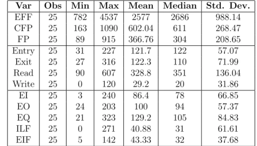
Table 1 shows some summary statistics related to the 25 Web applica-tions employed in our study3. The variables are EFF, i.e., the actual effort
expressed in terms of person-hours, CFP, expressed in terms of number of COSMIC Function Points, and FP, expressed in terms of number of Function Points. Furthermore, we have reported the variables denoting the BFCs for COSMIC (Entry, Exit, Read, and Write), expressed in terms of number of COSMIC Function Points, and Function Points (i.e., EI, EO, EQ, ILF, and EIF), expressed in terms of number of unadjusted Function Points.
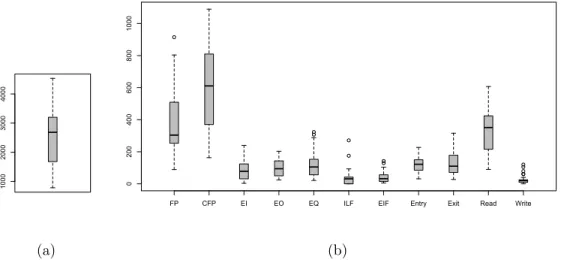
Figure 3 shows the boxplots of the distributions of these variables. We can observe that the boxplot of FP has one outlier and the box length and tails are more skewed than those of the boxplot of CFP. The figure also highlights that EFF has a different distribution with respect to CFP and FP. As for the single BFCs of COSMIC, we can note that the boxplots for Read and Exit are more skewed than the boxplots of Entry and Write. They have no outliers. Regarding the single BFCs of Function Points, the boxplots for EQ, ILF, and EIF have outliers and are more skewed than the boxplots of EI and EO.
3Raw data cannot be revealed because of a Non Disclosure Agreement with the software
Table 1: Descriptive statistics of EFF, CFP, FP, Entry, Exit, Read, Write, EI, EO, EQ, ILF, and EIF
.
Var Obs Min Max Mean Median Std. Dev.
EFF 25 782 4537 2577 2686 988.14 CFP 25 163 1090 602.04 611 268.47 FP 25 89 915 366.76 304 208.65 Entry 25 31 227 121.7 122 57.07 Exit 25 27 316 122.3 110 71.99 Read 25 90 607 328.8 351 136.04 Write 25 0 120 29.2 20 31.86 EI 25 3 240 86.4 78 66.85 EO 25 24 203 100 94 57.37 EQ 25 21 323 129.2 105 84.83 ILF 25 0 271 40.88 31 61.61 EIF 25 5 142 43.33 32 37.68
3.1.2. Selected estimation methods
In our empirical analysis we employed as estimation techniques SLR, that is a model-based approach, and CBR, that is a Machine Learning-based solu-tion, since they have been widely and successfully employed in the industrial context and in several researches to estimate development effort (see e.g., [12] [17] [37] [49] [54] [55] [56]).
SLR allows us to build estimation models to explain the relationship between the independent variable, denoting the employed size measure, and the dependent variable, representing the development effort. Thus, SLR allows us to obtain models of this type:
EF F =a+b∗Size (1)
whereEF F is the dependent variable,Sizeis the independent variable (i.e., CFP or FP),bis the coefficient that represents the amount the variableEF F changes when the variable Size changes 1 unit, anda is the intercept. Once such a model is obtained, given a new software project for which an effort estimation is required, the project manager has to size it using the same unit of measure of the model, and to use this value in the regression equation to get the effort prediction.
CBR is an alternative solution to SLR. It is a Machine Learning technique that can be used for classification and regression. In the domain of effort estimation, it allows us to predict the effort of a new project (target case) by considering some similar applications previously developed, representing
1000
2000
3000
4000
(a)
FP CFP EI EO EQ ILF EIF Entry Exit Read Write
0 200 400 600 800 1000 (b)
Figure 3: The boxplot of EFF (a) and FP, EI, EO, EQ, ILF, EIF, CFP, Entry, Exit, Read, and Write (b)
the case base (see e.g., [56]). In particular, similarly to SLR, once the new application is measured in terms of CFP or FP, the “similarity” between the target case and the other cases is measured, and the most similar past project (or more than one) is used, possibly with adaptations, to obtain the new effort estimation. To apply CBR, the project manager has to select an appropriate similarity function, the number of similar projects (analogies) to consider for the estimation, and the analogy adaptation strategy for generating the estimation.
In Sections 3.2.1 and 3.2.2 we provide the information on how we applied SLR and CBR in our study.
3.1.3. Validation method and evaluation criteria
In our analysis, we carried out an assessment to verify whether or not the obtained effort predictions are useful estimations of the actual development effort. To this end, we applied a cross-validation, splitting a data set into training and validation sets. Training sets are used to build the estimation models with SLR or to represent the case base when applying CBR, and validation sets are used to validate the obtained effort predictions. In par-ticular, we exploited a leave-one-out cross-validation, which means that the original data set is divided into n=25 different subsets (25 is the size of the
original data set) of training and validation sets, where each validation set has just one observation. This validation method is widely used in empirical studies when dealing with small data sets. Furthermore, a recent study has shown advantages of leave-one-out cross-validation with respect to K-fold cross-validation to assess software effort models [57].
Regarding the evaluation criteria, we exploited Absolute Residuals (AR), i.e., |Actual - Predicted|, where Actual is the actual effort and P redicted is the estimated effort, and to have a summary measure to accomplish the comparison among different estimation approaches we employed Median of AR (MdAR) since it is less sensitive to extreme values with respect the Mean of AR [58]. We also reported other summary measures, namely MMRE, MdMRE, Pred(25), that have been widely employed for effort estimation. However, they are reported only to allow for a comparison with previous researches published in this context and they are not used for the assessment of the achieved effort estimations. Indeed, the use of MMRE, and related measures, has been strongly discouraged in recent simulation studies, showing that MMRE wrongly prefers a model that consistently underestimates [59].
We also complemented the use of MdAR with the analysis of the box-plots of z, where z = P redictedActual , and boxplots of the residuals as suggested by Kitchenham et al. in [60]. Boxplots are widely employed in exploratory data analysis since they provide a quick visual representation to summarize the data using five values: median, upper and lower quartiles, minimum and maximum values, and outliers.
Moreover, we tested the statistical significance of the obtained results by using absolute residuals, to establish if COSMIC provided significantly better effort estimations than those achieved using FPA [60]. In particular, we performed the T-test (and the Wilcoxon signed rank test when absolute residuals were not normally distributed)[61] to verify the following null hy-pothesis “the two considered populations of absolute residuals have identical distributions”.
In order to have also an indication of the practical/managerial signifi-cance of the results, we verified the effect size. Effect size is a simple way of quantifying the standardized difference between two groups. It is a good complement to the tests of statistical significance, since “whereas p-values reveal whether a finding is statistically significant, effect size indicates prac-tical significance” [62]. In particular, we employed the Cliffsdnon-parametric effect size measure because it is suitable to compute the magnitude of the difference when a non parametric test is used [62]. In the empirical software
engineering field, the magnitude of the effect sizes measured using the Cliffs d can be classified as follows: negligible (d <0.147), small (0.147 to 0.33), medium (0.33 to 0.474), and large (d >0.474) [62].
3.2. Results of the empirical study
We first report on the application of COSMIC and FPA in combination with SLR (Section 3.2.1) to estimate Web application development effort and then the results obtained using CBR as estimation technique (Section 3.2.2). 3.2.1. Empirical results with SLR
We performed the SLR analysis to build the effort estimation models by using the data set of 25 Web applications of Table 1. To this end, we first verified the linear regression assumptions, i.e., the existence of a linear relationship between the independent variable and the dependent variable (linearity), the constant variance of the error terms for all the values of the independent variable (homoscedasticity), the normal distribution of the error terms (normality), and the statistical independence of the errors, in particular, no correlation between consecutive errors (independence).
In the following, we report on the analysis carried out to verify these assumptions. Note that the results of all the performed tests are intended as statistically significant at α=0.05 (i.e., 95% confidence level).
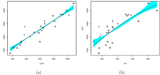
• Linearity. Figure 4(a) illustrates the scatter plot obtained by consid-ering EFF and CFP. We can observe that the scatter plot shows a positive linear relationship between the involved variables. The lin-ear relationship was also confirmed by the Plin-earson’s correlation test (statistic=0.932 with p-value <0.01) [63] and the Spearman’ rho test (statistic=0.942 with p-value <0.01) [61]. As for FP, from the scat-ter plot in Figure 4(b) we can observe a positive linear relationship with the variable EFF. The linear relationship was also confirmed by the Pearson’s correlation test (statistic=0.782 with p-value <0.01) [63] and the Spearman’ rho test (statistic=0.8 with p-value <0.01) [61]. These results also allow us to verify that CFP is more monotonously correlated with EFF than FP.
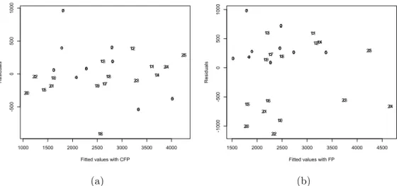
• Homoscedasticity. From the scatter plot shown in Figure 5 we can ob-serve that the residuals fall within a horizontal band centered on 0, for both CFP and FP. However, some outliers may be noted, e.g., observa-tions 7 and 16 for CFP and observaobserva-tions 7, 20, and 22 for FP. Thus, we
further investigated the homoscedasticity assumption by performing a Breush-Pagan Test [64], with the homoscedasticity of the error terms as null hypothesis. This assumption is verified for the CFP, since the p-value (0.741) of the statistic (0.110) is greater than 0.05 and therefore the null hypothesis cannot be rejected. As for the FP, the null hypoth-esis cannot be rejected since p-value (0.44) of the statistic (0.596) was greater than 0.05.
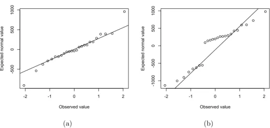
• Normality. The analysis of Normal Q-Q plot for CFP in Figure 6(a) revealed that only some observations were not very close to the straight line and they should get closer attention (“outliers”). As for FP, the Normal Q-Q plot in Figure 6(b) was characterized by an S-shaped pat-tern revealing that there are either too many or two few large errors in both directions, i.e., the residuals have an excessive kurtosis [65]. Thus, in order to verify the normality assumption, we also used the Shapiro-Wilk Test [66], by considering as null hypothesis the normality of error terms. The results of the test for CFP revealed that the assumption can be considered to be verified since the p-value (0.389) of the statistic (0.959) was greater than 0.05 and thus the null hypothesis cannot be rejected. Differently, for FP the null hypothesis can be rejected since the p-value (0.022) of the statistic (0.904) was less than 0.05.
• Independence. The uncorrelation of residuals for consecutive errors has been verified by a Durbin-Watson statistic. For CFP the test provided a value quite close to 2 (1.543) and p-value (0.109) greater than 0.05, thus, we can assume that the residuals are uncorrelated. Differently, in the case of FP the test highlighted minor cases of positive serial correlation since a value not very close to 2 (1.207) was obtained with a p-value (0.0128) less than 0.05.
Taking into account the results of the performed analysis to verify linear regression assumptions (in particular, for the Normality and Independence) we decided to apply a log transformation to the variables in order to avoid an unfair comparison between CFP and FP in predicting development effort. The variables log transformed are denoted as Log(CFP) and Log(FP).
We also verified the presence of influential data points (i.e., extreme val-ues which might unduly influence the models obtained from the regression analysis). As suggested in [67], we further analyzed the residuals plot and
200 400 600 800 1000 1000 2000 3000 4000 CFP EF F 1 2 3 4 5 6 7 8 9 10 11 12 13 14 15 16 17 18 19 20 21 22 23 24 25 (a) 200 400 600 800 1000 2000 3000 4000 FP EF F 1 2 3 4 5 6 7 8 9 10 11 12 13 14 15 16 17 18 19 20 21 22 23 24 25 (b)
Figure 4: The scatter plot for EFF and CFP (a) and EFF and FP (b), resulting from the SLR
used Cook’s distance to identify possible influential observations. In partic-ular, the observations in the training set with a Cook’s distance higher than 4/n (where n represents the total number of observations in the training set) were removed to test the model stability, by observing the effect of their removal on the model. If the model coefficients remained stable and the ad-justed R2 improved, the highly influential projects were retained in the data analysis. Figure 5(a) suggests that two observations seemed to have a large residual (i.e., observations 7 and 16). For observation 7, the Cook’s distance was greater than 4/25, indicating that it was an influential observation, while for 16 the distance was less than 4/25. To check the model’s stability, a new model was generated without observation 7. In the new model the indepen-dent variable remained significant, the adjusted R2 improved a little, and the coefficient present similar value to the one in the previous model. Thus, the observation was not removed [67].
We also verified the presence of influential data points for the variable FP having residuals far from the horizontal band centered on 0 (see Figure 5(b)). This analysis revealed that observation 24 was characterized by a Cook’s distance greater than 4/25. A new model was generated without observation 24 in the data set, which presented a coefficient similar to the one in the previous model and had a better adjusted R2. So, no observation
1000 1500 2000 2500 3000 3500 4000 -5 00 0 500 1000
Fitted values with CFP
R esi du al s 1 2 3 4 5 6 7 8 9 10 11 12 13 14 15 16 17 18 19 20 21 22 23 24 25 (a) 1500 2000 2500 3000 3500 4000 4500 -1 00 0 -5 00 0 500 1000
Fitted values with FP
R esi du al s 1 2 3 4 5 6 7 8 9 10 11 12 13 14 15 16 17 18 19 20 21 22 23 24 25 (b)
Figure 5: The scatter plot for residuals and predicted values for CFP (a) and FP (b), resulting from the application of SLR
was removed from the data set.
Table 2 shows some statistics about the model obtained with SLR by considering Log(CFP) as independent variable. A high R2 value (and cor-responding adjusted R2 value) is an indicator of the goodness of the model,
since it measures the percentage of variation in the dependent variable ex-plained by the independent variable. Other useful indicators are the F-value and the corresponding p-value (denoted by Sign. F), whose high and low values, respectively, denote a high degree of confidence for the prediction. Moreover, we performed a t-statistic and determined the p- and the t-values of the coefficient and the intercept in order to evaluate their statistical sig-nificance. A p-value less than 0.05 indicates that we can reject the null hypothesis and the variable is a significant predictor with a confidence of 95%. As for the t-value, a variable is significant if the corresponding t-value is greater than 1.5.
The equation of the regression model obtained for Log(CFP) is:
Log(EF F) = 2.74 + 0.8∗Log(CF P) (2) and when it is transformed back to the original raw data scale we obtain:
-2 -1 0 1 2 -5 00 0 500 1000 Observed value Exp ect ed n orma l va lu e (a) -2 -1 0 1 2 -1 00 0 -5 00 0 500 1000 Observed value Exp ect ed n orma l va lu e (b)
Figure 6: The Q-Q plot for residuals for CFP (a) and FP (b), resulting from the application of SLR
Table 2: The results of the SLR analysis with COSMIC on Log(CFP)
Variable Value Std. Err t-value p-value
Coefficient 0.8 0.06 12.64 <0.01
Intercept 2.74 0.4 6.87 <0.01
R2 Adjusted R2 Std. Err F Sign. F
0.87 0.87 0.16 159.8 <0.01
We can observe that the model described by Equation 2 is characterized by a highR2 value (0.87), a highF value (159.8), and a low p-value (<0.01), indicating that a prediction is possible with a high degree of confidence (see Table 2). The t-values and p-values for the corresponding coefficient and the intercept present values greater than 1.5 and less than 0.05, respectively. Thus, the predictors can be considered important and significant.
Table 3 shows the results of the application of the SLR by considering Log(FP) as independent variable. We can observe that the coefficient and the intercept can be considered accurate and significant as from the t-statistic, but the R2 and F values are lower than those obtained with Log(CFP).
To evaluate the prediction accuracy of the models obtained with SLR, we performed the leave-one-out cross-validation, whose results are reported
Table 3: The results of the SLR analysis with Function Points on Log(FP)
Variable Value Std.Err t-value p-value
Coefficient 0.56 0.12 4.53 <0.01
Intercept 4.47 0.73 6.12 <0.01
R2 Adjusted R2 Std. Err F Sign. F
0.47 0.45 20.55 0.33 <0.01
Table 4: The results of the validation for SLR
Variable MdAR MMRE MdMRE Pred(25)
CFP 180 0.12 0.07 0.92
FP 515 0.29 0.18 0.68
in Table 44. We can observe that the MdAR value achieved with the CFP
based model is more than two times lower than the one obtained with the FP based model, thus highlighting much better results with COSMIC.
These results are confirmed by the boxplots of residuals and of z shown in Figure 7. Indeed, even if the boxplot of residuals for CFP has two outliers, its median is closer to zero. Moreover its box length and tails are less skewed than those of the boxplot of residuals for FP (see Figure 7(a)). As for boxplots of z, CFP has a median closer to 1 and again the box length and tails are less skewed than those of FP (see Figure 7(b)).
This finding is corroborated by the tests on the statistical significance of the results by using absolute residuals [49] [60]. In particular, the Wilcoxon test revealed that the estimations obtained with CFP are significantly bet-ter than those obtained with FP (p-value < 0.01) with a large effect size (d=0.63). Observe that we applied the Wilcoxon test since the absolute residuals obtained with CFP were not normally distributed, as highlighted by the Shapiro test (p-value < 0.01).
3.2.2. Empirical results with CBR
Before applying CBR, we verified which one of the two variables FP and CFP is more informative for EFF, by considering the correlation between distance matrices. A high correlation between distances of EFF values and distances of CFP values can indicate that projects similar according to
CFP FP -1 00 0 -5 00 0 500 1000 (a) CFP FP 0.5 1.0 1.5 2.0 (b)
Figure 7: The boxplots of residuals (a) and z (b) obtained with SLR
MIC size are similar according to effort. To this end, we applied the Mantel test [68], which checks the correlation between two distance matrices. It is a non-parametric test that computes the significance of the correlation through permutations of the rows and columns of one of the input distance matrices. The test statistic is the Pearson product-moment correlation coefficient r. The values for r can fall in the range of -1 to +1, where being close to -1 indicates strong negative correlation and +1 indicates strong positive corre-lation. An r value of 0 indicates no correlation. In particular, we performed the Mantel test by considering the null hypothesis that the two matrices, i.e., the EFF distances and the CFP distances, are unrelated. Similarly, we performed the test considering as matrices the EFF distances and the FP distances. For both CFP and FP, the results of the test revealed that we can reject the null hypothesis that the correlation matrices are unrelated since we obtained p-values less than 0.05. In the case of EFF and CFP distances, we obtained r = 0.824, while in the case of EFF and FP distances, the test was characterized byr=0.579. Thus, the correlation matrix entries are positively associated and CFP is more informative for EFF than FP.
In order to apply CBR we exploited the tool ANGEL [56] that implements the Euclidean distance as similarity function using variables normalized be-tween 0 and 1 and allows users to choose the relevant features/predictors, the number of analogies, and the analogy adaptation technique for
generat-ing the estimations. As for the predictors, we used the variables CFP and FP. The selection of the number of analogies is a key task, since it refers to the number of similar cases to use for estimating the effort required by the target case. Since we dealt with a not so large data set, we used 1, 2, and 3 analogies, as suggested in many similar works (see e.g., [49]). To obtain the estimation once the most similar cases were determined, we employed three widely adopted adaptation strategies: the mean of k analogies, i.e., simple average, the inverse distance weighted mean (see e.g., [49] [69]), and the inverse rank weighted mean (see e.g., [56]). So, performing a leave-one-out cross-validation, we obtained 25 estimations and the corresponding residuals, for each selection of the number of analogies and of the analogy adaptation techniques. Indeed, each estimate was achieved by selecting an observation from the whole data set of 25 Web applications (in Table 1) as validation set and employing the remaining observations (i.e., 24) as training set. This was performed 25 times.
Table 5 shows the results obtained with CBR. We can observe that the MdAR values achieved with CFP are much better than those achieved with FP for all the considered configurations. Furthermore, the best result achieved with CFP (i.e., with k=3 as number of analogies and mean of k analogies as adaptation strategy) is two times lower than the best result obtained with FP (i.e., with k=3 as number of analogies and inverse rank weighted mean as adaptation strategy). Similarly to the SLR results, the boxplots of residuals and z for CFP have box length and tails less skewed than those of the boxplots of residuals for FP (see Figure 8(a) and (b)).
These results are corroborated by the tests on the statistical significance of the results by using absolute residuals [49] [60]. In particular, we com-pared the absolute residuals achieved with CFP using k=3 as number of analogies and mean of k analogies as adaptation strategy and the absolute residuals obtained with FP using k=3 as number of analogies and inverse rank weighted mean as adaptation strategy. The results of the Wilcoxon test revealed that the estimations obtained with CFP are significantly better than those obtained with FP (p-value=0.03) with a small effect size (d=0.19).
Thus, the results with CBR confirm that CFP leads to better effort pre-dictions than FP.
We can also observe that CBR provided slightly worse results than SLR, in terms of MdAR (see Tables 4 and 5). This result is confirmed by the anal-ysis of the boxplots of residuals and z. The statistical analysis performed on absolute residuals revealed that the difference in the absolute residuals
ob-Table 5: The results of the validation for CBR
CBR with MdAR MMRE MdMRE Pred(25)
Using CFP as predictor
k=1; mean of k analogies 362 0.17 0.12 0.80
k=2; mean of k analogies 245 0.16 0.12 0.80
k=3; mean of k analogies 218 0.15 0.10 0.84
k=1; inverse distance weighted mean 362 0.18 0.12 0.80
k=2; inverse distance weighted mean 262 0.16 0.11 0.88
k=3; inverse distance weighted mean 282 0.15 0.12 0.88
k=1; inverse rank weighted mean 362 0.18 0.12 0.80
k=2; inverse rank weighted mean 291 0.16 0.12 0.88
k=3; inverse rank weighted mean 286 0.15 0.12 0.88
Using FP as predictor
k=1; mean of k analogies 535 0.44 0.19 0.56
k=2; mean of k analogies 576 0.32 0.21 0.52
k=3; mean of k analogies 449 0.32 0.20 0.60
k=1; inverse distance weighted mean 535 0.44 0.19 0.56
k=2; inverse distance weighted mean 470 0.35 0.20 0.60
k=3; inverse distance weighted mean 468 0.35 0.20 0.64
k=1; inverse rank weighted mean 535 0.44 0.19 0.56
k=2; inverse rank weighted mean 435 0.35 0.18 0.68
k=3; inverse rank weighted mean 485 0.34 0.18 0.68
tained with the two techniques is not statistically significant (p-value=0.05), with a small effect size (d = 0.23), when using CFP as independent vari-able. However, note that the p-value is equal to the threshold 0.05. In the case of using FP, the p-value obtained with the Wilcoxon test is 0.56, so the difference in the absolute residuals achieved with the two techniques is not statistically significant. The effect size in this case is negligible (d=0.06). 3.3. Answering RQ1a
The results reported in Tables 4 and 5 suggest that, on our data set, CFP can be considered a good indicator of the development effort, when used in combination with the two analyzed estimation methods (i.e., SLR and CBR). Moreover, the effort estimates achieved with CFP are significantly better than those obtained with FP, with an improvement of 65%5 in terms
of MdAR value and a large effect size in the case of SLR. Thus, the software company involved in our study should profitably move from FPA to COSMIC to improve the quality of its effort estimations.
5The average percentage improvement has been calculated as (MdAR of the FP based
CFP FP -1 50 0 -5 00 500 1500 (a) CFP FP 0.5 1.0 1.5 2.0 2.5 (b)
Figure 8: The boxplots of residuals (a) and z (b) obtained with CBR
Summarizing, we can positively answer the first research question: COS-MIC measure is significantly better than FPs for estimating Web application development effort by simple linear regression and case based reasoning. 3.4. Answering RQ1b
To answer the second research question, we first verified the correlation between each BFC and the effort. To this aim, we applied the Spearman rho test, whose results are reported in Table 6.
We can observe that, as for COSMIC, all the four BFCs are statistically significant correlated with EFF since the p-values are less than 0.01. In particular, we can observe that three of them (i.e., Entry, Exit, and Read) have a rho statistic greater than 0.8 that can be considered a good value [61], while Write was characterized by a lower value. Among them, the Read BFC resulted to be the more informative one for EFF, having the highest rho statistic (0.919). This result is confirmed by the analysis of the distribution of the BFCs with respect to the final size, whose results are reported in Table 6. These results are in line with the type of Web applications we dealt with. Indeed, the applications in our data set mainly provide information to the users, by requiring many queries to the persistent layers of the applications, being counted in COSMIC as Reads.
Table 6: Correlation among EFF and each BFC of the COSMIC and FPA method
BFC rho statistic p-value
Entry 0.823 <0.01 Exit 0.859 <0.01 Read 0.919 <0.01 Write 0.535 <0.01 EI 0.741 <0.01 EO 0.324 0.11 EQ 0.671 <0.01 ILF 0.321 0.118 EIF 0.141 0.5
From these results we can conclude that: all the COSMIC BFCs are significantly correlated with EFF and Read resulted to be the one more infor-mative for predicting EFF.
The same kind of analysis has been performed for FPs, revealing that only EI and EQ are statistically significant correlated with EFF (see the results of the Spearman rho test reported in Table 6). In particular, EI resulted to be the more informative for EFF (rho statistic = 0.741), but its statistic does not reach the level of 0.8. The analysis of the distribution of the Function Point BFCs with respect to the EFF suggests that the main contribution to the final size comes from EQ, EO, and EI. This leads to the same kind of observations done for COSMIC on the prevalent type of operations in the considered Web applications. Nevertheless, these lower values confirm that FPA is missing to fully capture the size of a Web application. Moreover, these results further suggest that COSMIC, and its single BFCs, are more informative for EFF than FPs and its single BFCs, for the considered kind of Web applications
From these results we can conclude that: only EI and EQ are significantly correlated with EFF among the FP BFCs and EI resulted to be the more informative for predicting EFF.
4. The Second Empirical Study: Assessing the use of 2SEP
From the results of our first empirical study, it is clear that the software company in our study can benefit from migrating to COSMIC, since on the considered projects this method provided significantly better development
Table 7: Distribution of the BFCs with respect to the final size in terms of CFP
FSM method Entry Exit Read Write
COSMIC 20% 19% 56% 5%
FSM method EI EO EQ ILF EIF
FPA 22% 25% 32% 10% 11%
effort estimates. Our second empirical study aims at understanding how eas-ily this migration can be achieved. As mentioned in the introduction of this paper, a company interested in the adoption of COSMIC has to build an estimation model with this measure. This basically requires historical data based on COSMIC that can be obtained by manually remeasuring all the ap-plications previously developed. This task not only requires a lot of time, but in some cases might not even be possible (e.g., due to the lack of appropriate documentation). The reuse of data based on FPA could be very valuable to address the problem, provided that there is a way to obtain the size in terms of CFPs from the size in terms of FPs. As it was pointed out by Abran et al. [53], FPA and COSMIC measures focus on different aspects of software systems since they are based on different basic functional components. Thus, “exact mathematically-based conversion formulae from sizes measured with a 1st generation method to COSMIC sizes are impossible”. A possible way to address the problem, also suggested in the COSMIC documentation [53], is to search for some “statistically-based conversion formulae”.
Some researchers have been investigating the suitability and the effective-ness of such an approach by trying to build conversion equations for different data sets. In particular, linear and non-linear equations have been built on the raw data and on the log-transformed data, respectively [14]. Also, more sophisticated techniques, such as piecewise regression, have been employed for building non-linear models [15].
The results reported in the literature [14] [15] [22] [23] [70] [71] [72] [73] [74] reveal that a statistical conversion is possible, thus supporting the sugges-tions provided in the COSMIC documentation [53]. The studies also showed that both linear and non-linear models should be analyzed to identify the best correlation. Furthermore, more complex techniques, such as piecewise regression [15]), did not provide significantly better results, being at the same time hardly applicable.
possi-ble to reuse the FP → CFP conversion equations proposed in the literature (i.e., external conversion equations) to apply the two-step process shown in Figure 1 (named 2SEP) for building effort estimation models. In other words, we assessed if, given the size of past projects in terms of FPs, it is possible to convert them by means of some equations into COSMIC measure to build an effort estimation model. Furthermore, we also considered the use of conver-sion equations built on a (small) data set of the company taken into account (i.e., internal conversion equations).
In the following, before presenting the design (Section 4.3) and the results (Section 4.4) of our second empirical study, we provide a brief description of the external conversion equations we decided to employ (Section 4.1) and we describe the construction of the internal conversion equations (Section 4.2). 4.1. External conversion equations from previous studies
In our study we took into account the results of two previous investiga-tions that analyzed the relainvestiga-tionship between the sizes expressed in terms of FPs and of CFPs, namely [14] and [75].
The aim of Cuadrado-Gallego et al. [14] was to carry out a review of previous investigations that mainly exploited linear regression analysis for converting FPs into CFPs, i.e., by constructing an equation as:
CF PF P =a+b∗F P (4)
where the dependent variable CFPF P represents the estimated COSMIC size and the independent variable FP represents the size in terms of FPs.
Moreover, Cuadrado-Gallegoet al. were also the first to propose an anal-ysis on a non-linear relation between CFPF P and FP, by exploiting the log transformation of the variables in the application of linear regression analysis. Thus, the equation obtained is of this form:
Log(CF PF P) =Log(a) +b∗Log(F P) (5) which, when transformed back to the original raw data scale, gives the equa-tion:
CF PF P =a∗F Pb (6)
For the evaluation, they employed nine publicly available data sets: six of them were obtained from previous studies (i.e., named fet99[76],fet99-2[77], ho99[71], vog03[77], abr05[22], and des06[23]). Three additional data sets
Table 8: Parameters of the equations in [14]
Linear
Data set fet99 fet99-2 ho99 vog03 abr05 des06 jjcg06 jjcg07 jjcg0607
b 1.12 1.14 1.03 1.2 0.84 1 0.82 0.86 0.69
a -6.23 -7.6 -6.6 -86.8 18 -3.23 -36.6 0.19 13.04
R2 0.98 0.97 0.98 0.99 0.91 0.93 0.7 0.86 0.85
Non-Linear
Data set fet99 fet99-2 ho99 vog03 abr05 des06 jjcg06 jjcg07 jjcg0607
b 1.11 1.12 1.14 1.18 0.96 1.07 1.17 1.02 0.9
a 0.64 0.62 0.52 0.28 1.08 0.67 0.27 0.75 1.26
R2 0.99 0.97 0.99 0.94 0.88 0.95 0.82 0.73 0.87
were included in the paper: the first two (namedjjcg06 andjjcg07) contained 21 and 14 observations, respectively, and were obtained in two different stud-ies conducted with academic students, while the third one (named jjcg0607) was obtained by merging the first two.
The parameters of the linear and non-linear conversion equations obtained for the above data sets are reported in Table 86, respectively. In particular,
the tables show, for each employed data set, the equation parameters a and b, and the R2 value. We can observe that the linear conversion equations re-ported in Table 8 (top) are characterized by a coefficient quite close to 1, and the non-linear equations (see Table 8 (bottom)) have the coefficient values even closer to 1. These results seem to suggest that a conversion equation based on the assumption of 1 CFP ∼= 1 FP could be possible. Cuadrado-Gallego et al. argued that a 1 to 1 conversion factor cannot be attributed to anything other than an influential coincidence. Indeed, even if both FPA and COSMIC measure the functional size of the software, they are taking in consideration different characteristics and also different counting procedures. [14].
Lavazza [75] also exploited some of the data used in previous work [14][47] to empirically assess and compare linear and non-linear models against Piece-wise Linear Regression, with a special emphasis on the role of outliers. He built 6 linear and 6 non-linear models, whose information can be found in
6Note that we applied the procedure employed in [14] for building the conversion
equa-tions exploiting the data sets that they published and in 5 cases (namely jjcg0607 linear and non-linear, ho99 non-linear, vog03 non-linear) we found some differences in the ob-tained models with respect to [14]. In the table we report the values we obob-tained.
Table 9: Parameters of the equations in [75]
Linear
Data set vog03 des06 vanH07 jjcg06 jjcg07 jjcg0607
b 0.78 0.97 1.05 0.7 0.86 0.65
a -3.8 -5.9 -17.9 -2.4 0.2 19.07
R2 0.94 0.97 0.95 0.65 0.86 0.85
Non-Linear
Data set vog03 des06 vanH07 jjcg06 jjcg07 jjcg0607
b 1.2 1.03 1.09 1.62 1.12 0.97
a 0.28 0.84 0.61 0.27 0.46 0.87
R2 0.98 0.97 0.95 0.82 0.83 0.93
Table 9. These equations differ from the one in the work of Cuadrado-Gallego et al. [14] since Lavazza eliminated from the data sets the outliers affecting the models. As already mentioned at the beginning of Section 4, we did not consider the Piecewise Regression since it did not provide significantly better results than SLR, being at the same time hardly applicable [15].
4.2. Internal conversion equations built on our data set
To build internal conversion equations with SLR we first verified the relationship between the dependent and independent variables CFP and FP, respectively, by assessing linear regression assumptions, i.e., linearity, homoscedasticity, normality, and independence. In particular, the Spear-man’ rho test revealed that there was a positive linear relationship between CFP and FP (statistic=0.848 with p-value <0.01), while the Breush-Pagan Test showed that homoscedasticity assumption was verified since the p-value (0.674) of the statistic (0.176) was greater than 0.05. On the other hand, the normality assumption for the residuals cannot be considered to be verified since the p-value (0.243) of the statistic (0.949) was greater than 0.05. As for the independence, the Durbin-Watson statistic was not close to 2 (1.34). As a consequence, we also applied a log-transformation of the data and we con-sidered both linear and non-linear conversion equations as done in previous investigations (e.g., [14], [75]).
Since we were interested to verify the possibility for the company involved in our study to build its own convertibility equation using a small sample of projects from their own organization instead of using someone else equations,
we employed a data set of 5 observations7.
4.3. Design of the study
The empirical study performed to answer research questions RQ2a and RQ2b employs the same data set used in the first empirical study (see Section 3.1.1), whose descriptive statistics are shown in Table 1.
For the application of 2SEP we have to select an FP → CFP conver-sion equation and a model building technique to obtain the effort estimation model. We employed both external and internal conversion equations. Re-garding the model building technique, we used SLR since in the first empirical study it performed better than CBR (see Section 3.3). We verified linear re-gression assumptions for each built model and as a result we performed a log transformation of the dependent and independent variables employed, as done for the first research question.
When exploiting external conversion equations, we used those reported in Tables 8 and 9. Moreover, given its immediate applicability, we also investi-gated 2SEP using a 1 to 1 conversion factor (named from here on 1-1 Conv). Thus, as first step of 2SEP, we exploited 15 linear, 15 non-linear and the 1-1 Conv conversion equations, to obtain 31 new data sets, where the 25 Web applications are expressed in terms of estimated CFPs. Then, as second step of 2SEP, we applied SLR on each of them and obtained estimation models of this type: EF F = a∗(CF PF P)b, where EF F is the dependent variable and CF PF P is the independent variable. As mentioned in previous section CF PF P represents the estimated COSMIC size through the chosen FP → CFP conversion equation.
Concerning the assessment of 2SEP with external conversion equations, we used again a leave-one-out cross-validation for each of the employed con-version equations. In particular, we simulated the situation where the com-pany has a historical data set of 24 projects (i.e., the training set) sized with FPA and the project manager is willing to estimate the effort for a new project (i.e., the validation set) sized with COSMIC. This setting reflects what could happen in reality in a software company willing to migrate from FPA to COSMIC. Thus, the effort predicted of a new project is obtained by giving as input to the estimation model EF F =a∗(CF PF P)b, built on the
7A rule of thumb in regression analysis is that 5 to 10 records are required for every
![Figure 2: The four types of Data Movements, and their relationship with a Functional Process [5]](https://thumb-us.123doks.com/thumbv2/123dok_us/10232706.2927175/10.918.266.657.198.391/figure-types-data-movements-relationship-functional-process.webp)