RENEWABLE ENERGY AND ELECTRICITY PRICES: INDIRECT EMPIRICAL
EVIDENCE FROM HYDRO POWER
Ronald Huisman, Victoria Stradnic, Sjur Westgaard
Document de treball de l’IEB
2013/24
Documents de Treball de l’IEB 2013/24
RENEWABLE ENERGY AND ELECTRICITY PRICES:
INDIRECT EMPIRICAL EVIDENCE FROM HYDRO POWER
Ronald Huisman, Victoria Stradnic, Sjur Westgaard
The
Barcelona Institute of Economics (IEB)
is a research centre at the University of Barcelona
(UB) which specializes in the field of applied economics. The
IEB
is a foundation funded by
the
following institutions: Applus, Abertis, Ajuntament de Barcelona, Diputació de Barcelona, Gas
Natural and La Caixa.
Within the IEB framework, the
Chair of
Energy Sustainability
promotes research into the
production, supply and use of the energy needed to maintain social welfare and development,
placing special emphasis on economic, environmental and social aspects. There are three main
research areas of interest within the program: energy sustainability, competition and consumers,
and energy firms. The energy sustainability research area covers topics as energy efficiency,
CO2 capture and storage, R+D in energy, green certificate markets, smart grids and meters,
green energy and biofuels. The competition and consumers area is oriented to research on
wholesale markets, retail markets, regulation, competition and consumers. The research area on
energy firms is devoted to the analysis of business strategies, social and corporative
responsibility, and industrial organization. Disseminating research outputs to a broad audience is
an important objective of the program, whose results must be relevant both at national and
international level.
The
Chair of
Energy Sustainability of the University of Barcelona-IEB
is funded by the
following enterprises ACS, CEPSA, CLH, Enagas, Endesa, FCC Energia, HC Energia, Gas
Natural Fenosa, and Repsol) through FUNSEAM (Foundation for Energy and Environmental
Sustainability).
Postal Address:
Chair in Energy Sustainability
Institut d’Economia de Barcelona
Facultat d’Economia i Empresa
Universitat de Barcelona
C/ Tinent Coronel Valenzuela, 1-11
(08034) Barcelona, Spain
Tel.: + 34 93 403 46 46
Fax: + 34 93 403 98 32
ieb@ub.edu
http://www.ieb.ub.edu
The IEB working papers represent ongoing research that is circulated to encourage discussion
and has not undergone a peer review process. Any opinions expressed here are those of the
Documents de Treball de l’IEB 2013/24
RENEWABLE ENERGY AND ELECTRICITY PRICES:
INDIRECT EMPIRICAL EVIDENCE FROM HYDRO POWER
*Ronald Huisman, Victoria Stradnic, Sjur Westgaard
ABSTRACT:
Many countries have introduced policies to stimulate the production of electricity in a sustainable or renewable way. Theoretical and simulation studies provide evidence that the introduction of renewable energy promotion policies lead to lower electricity prices as sustainable energy supply as wind and solar have very low or even zero marginal costs. Empirical support for this result is relatively scarce. The motivation for this study is to provide additional empirical evidence on how the growth of low marginal costs renewable energy supply such as wind and solar influences power prices. We do so indirectly studying Nord Pool market prices where hydro power is the dominant supply source. We argue that the marginal costs of hydro production varies depending on reservoir levels that determine hydro production capacity. Hydro power producers have an option to produce or to delay production and the value of the option to delay increases when the reservoir levels decrease and the option to delay decreases in value when reservoir levels increase and producers face the risk of spillovers. Hence, an increase in reservoir levels mimics the situation of an increase of low marginal costs renewable energy in a market. Our results show that higher reservoir levels, more hydro capacity, lead to significant lower power prices. From this we conclude that an increase in low marginal costs renewable power supply reduces the power prices. The second contribution of this paper is that we develop a market clearing price model by modelling the supply curve of power that varies over time depending on fundamentals such as hydro capacity and the prices of alternative power sources and that deals with maximum prices which apply to all power markets that we know. With our result, we strengthen support for the view that an increase in wind and solar supply lowers the power price. This is good news for consumers, but it increases the costs of sustainable energy policies such as feed-in tariffs and at the same time lowers revenues and profits for power producers in case governments would abandon such policies. This effect makes the economic and policy support for renewable energy less sustainable. Policy makers have to account for this if they want to stimulate a sustainable growth of sustainable energy supply.
JEL Codes: C51, Q41, Q42, Q48
Keywords: Energy policies, sustainable energy, market clearing price, supply curve model.
Ronald Huisman
Erasmus School of
Economics & IEB
P.O. Box 1738
3000 DR, Rotterdam, The
Netherlands,
E-mail:
rhuisman@ese.eur.nl
Victoria Stradnic
Erasmus School of Economics
P.O. Box 1738
3000 DR, Rotterdam, The
Netherlands,
E-mail:
stradnicv@gmail.com
Sjur Westgaard
Norwegian University of Science
and Technology
Sentralbygg I
1153 Alfred Getz vei 3, Trondheim,
Norway
E-mail :
sjur.westgaard@iot.ntnu.no
1
Introduction
Many countries have introduced policies to stimulate the production of electricity in a sustainable or renewable way1. The most popular policy is feed-in tariffs that provide green power producers a guaranteed price for their output. Under this policy, the government compensates a power producer for the difference between the guaranteed price and the market price of power. This policy reduces risk for sustainable energy producers and is therefore the most preferred policy by investors (Hofman and Huisman [2012]). By definition, a feed-in tariff policy becomes more expensive for a government when power prices decline as producers have to be compensated for a larger gap between the guaranteed price and the market price. Amundsen and Mortensen [2001], Jensen and Skytte [2002] and Fischer [2006] provide theoretical evidence that the introduction of renewable energy promotion policies has lead to lower electricity prices. These lower prices arise as sustainable energy supply as wind and solar have very low or even zero marginal costs as no fuel is needed to produce one additional unit of power. An increase of sustainable power supply in a price competitive energy market then results ultimately in lower energy prices. This effect introduces the following paradox. A feed-in tariff policy to stimulate sustainable energy becomes less sustainable in itself as the policy becomes more expensive when it successfully stimulates growth of renewable energy. Another implication of such a policy leading to lower power prices is that low energy prices reduce the revenues and profits for sustainable power producers in the case that a government would abandon the feed-in tariff policy and no longer compensates producers for the low energy prices. Sustainable energy then becomes less attrac-tive as an investment opportunity and therefore reduces the supply of private capital to finance sustainable energy production. The theoretical results that sustainable energy policies lead to lower energy prices have been confirmed by Sensfuss et al. [2008] and Linares et al. [2008] who provide insight from simulation studies.
Empirical support for this claim are relatively scarce possible due to a lack of data as it takes a long time before these policies result in a large enough share of sustainable energy to observe this effect in market prices. Yet, S´aenz de Miera et al. [2008], Jonsson at al. [2010], and Gelabert et al. [2011] have examined the impact of renewables on wholesale electricity prices and provide empirical prove for the claim. For instance, Gelabert et al. [2011] examine the Spanish market between 2005 and 2009 and report that a marginal increase of 1GWh of renewable electricity production and cogeneration yields a 4% decline in electricity prices.
The motivation for this study is to provide additional empirical evidence on how the growth in production from low marginal costs sustainable energy sources such as wind and solar influences power prices. We do so by not studying this relation directly such as relating power prices to wind and solar supply in some model. We take an different route that might provide insight from an alternative perspective. We focus on hydro power. Hydro producers convert stored water in reservoirs into power in volumes and at moments that they prefer. This amount of 1We will use the terms sustainable and renewable interchangeably regarding power production, although not
stored water in the reservoirs increase from rain fall, from melting snow or from water pumped from rivers into the reservoirs. We argue that we can learn about how the market clearing price changes when more low marginal costs supply is added to the market by examining the variation in reservoir levels and it’s impact on power prices. We reason that the marginal costs of hydro power production changes when the reservoir level changes. To see this, we see hydro capacity as a real option that hydro producers have to convert water into power. They decide to exercise the option to produce now based on the current power price and the expected opportunity loss that arises if they would use the water for producing at a later moment when prices might be higher. Therefore, the marginal costs of hydro power production is in fact equal to the value of a real option to delay production. This option is very valuable when the reservoir is almost empty. In this situation the marginal costs of hydro power is high as opportunity losses might be high as producing now implies an even lower inventory of water. The opposite holds when reservoirs are almost full. Torro [2007] states that hydro producers sell at lower prices when reservoirs are full as water may overflow which reduces the potential gains of producers. Hydro power producers are willing to sell against any (positive) price to prevent loosing water inventory from spill overs. Otherwise stated, the value of the real option to delay is almost zero. Therefore, the marginal costs of hydro production is low when reservoir levels are almost full and even zero when reservoir levels are full. Summarizing, the low marginal cost when the reservoirs are almost full is due to the low marginal value of water (worst case it must just flow out without any use). When the reservoirs are low, waiting to tap might be very profitable, hence the alternative cost is very high. This is particular true when it is a cold winter, when import is needed and coal/gas prices are high. We believe that the relation between marginal costs of hydro power production and reservoir levels can be used to examine what would happen to the market clearing price when more power supply from low marginal costs sources such as wind and solar is added to the market. An increase in the share of these power sources is comparable to an increase in reservoir levels as an increase in reservoir levels reduces the marginal costs of hydro production. This methodology has drawbacks off course as it doesn’t model the direct relation between wind and solar and energy prices. But the advantage of our approach is that we can learn by studying a mature market where there has been a major share of hydro production for a long time and therefore our results will suffer less from any effects due to changes in the supply side of the market. Hence, we believe that this methodology contributes to the empirical knowledge about the impact of renewable energy on energy prices. Our goal is therefore to empirically examine how the market clearing price changes in a market with hydro power when reservoir levels change. And according to the previous discussion, we expect that the adding more low marginal costs supply to the market (higher reservoir levels) lowers the market clearing price. To examine this, we construct a demand / supply model in which the supply curve is modeled as a function of reservoir level. We choose for this way of modeling instead of a direct (linear) regression analysis because we expect non linearities as the market clearing price might change due to variation in the level and convexity of the power supply curve due to variation in reservoir levels, consumption and prices of alternative power supply. This model is developed in the next section.
Our results show that variation in reservoir levels significantly change the level and convexity (price elasticity) of the power supply curve and therefore the market clearing price. For all consumption levels that we have observed in our Nord Pool sample, we show that an increase in reservoir level lowers power prices. And from this we conclude that more sustainable low marginal costs energy supply will reduce energy prices as an increase in reservoir levels is equivalent to an increase in low marginal costs supply in an energy market.
2
A demand and supply model for electricity
The market price of electricity in day-ahead and intra-day or imbalance markets is the outcome of the intersection of aggregated demand and supply stack submitted by electricity traders. Bar-low [2002] and Bozoianu et al. [2005] model electricity market (wholesale) prices by specifying demand and supply curves and a stochastic demand process. They show that most characteris-tics of electricity prices, such as mean-reversion, time varying volatility and price spikes, can be explained by the combination of demand dynamics and the (time varying) structure of supply and demand curves.
Barlow [2002] assumes that supply is non random and independent of time. This a strong assumption that does not necessarily apply to electricity markets. For instant, the Nord Pool market, the market which prices we examine in this paper, depends to a large extend on supply from hydro producers. The amount of hydro capacity varies over time due to variation in the level of water available in reservoirs. Reservoir levels depend on rain fall and temperature, which determines the in-flow of water from melting snow. Hydro power capacity therefore varies over time and it does so in a forecastable (as weather patterns are forecastable) and stochastic (fore-cast errors) way. Reservoir levels thus determine supply capacity and it is very likely that the structure of the supply curve varies over time as a consequence. Bozoianu et al. [2005] make a similar observation and argue that the structure of the supply curve in the Californian power market varies over time due to varying capacity of non fuel based power supply, variation in gas prices, and power plant outages. As we are interested to examine how reservoir levels influence the market clearing price through the supply curve, we follow Bozoianu et al. [2005] and assume that supply curve may vary over time in such a way that the shape of the supply curve depends on available hydro power capacity (reservoir levels).
Barlow [2002] and Bozoianu et al. [2005] model the supply curve as a function of price: the quantity offered given a price. Barlow [2002] uses a power function to structure the supply curve and Bozoianu et al. [2005] use an exponential function. We prefer the power function2.
Our preference is based on that power prices exhibit spikes, sudden high or low prices, and, as a consequence, the price distribution function is fat tailed. We think that the power function, with power decay in the tails3, models the tails better than the exponential function. We differ from both studies as we model, for reasons of mathematical convenience, the supply curve as a
2
We have applied the exponential as well yielding similar results as to what we will present later.
3
function of quantity: the price charged given a specific quantity. This is in fact the inverse of the supply curve as modeled by Barlow [2002] and Bozoianu et al. [2005]. As long as this inverse exists, which we assume4, we believe that this assumption does not seriously influence our results.
We examine day-ahead prices: price of contracts that deliver power during one specific hour in the following day5. Letpt(st) represent the supply curve: the price quoted on day t for delivery of st MW of power during hour h in day t + 16. We use the subscript t in pt to stress that we allow the structure of the supply curve to vary over time. The power supply curve that we, based on Barlow [2002] suggest is
pt(st) = ¯p−at(¯s−st)α, (1) where ¯p is the maximum price that can be set and ¯s is maximum installed supply capacity. The maximum price ¯p is an important feature as all power markets that we know apply a maximum price that can be quoted. In Nord Pool, the maximum price is AC2,000 per MWh7. We think it’s important to include this in the model as traders keep the maximum price in mind when supplying their bids and offers. In the remainder, we set ¯p = 2,000. The maximum installed supply capacity ¯s sets the physical limit of the market. It is likely that the maximum installed capacity varies over time, both in the short run (as a consequence of variations in the amount of water in hydro reservoirs for instance) and in the long run, but we assume it to be constant in this paper. We have set the maximum supply capacity at ¯s = 100,000 MW, a volume that has not been reached in the data sample that we use8.
The parametersat andαdetermine the structure of the supply curve. In order to have a supply curve which is convex and increasing, we need to have thatp0t(st)>0 and p
00
t(st)>0. The first and second order derivatives arept0(st) =αat(¯s−st)α−1andp0t(st) =−(α−1)αat(¯s−st)α−2. It can be shown easily that the following restrictions yield an increasing and convex supply curve: 0≤α≤1 andat ≥0.
The expressions for the first and second order derivatives show that both parameters at and α determine the first and second order derivative, in other words the slope and convexity of the supply curve. This is the reason why we choose the parameter αto be constant over time and to make at time-varying. That is, time-variation in the slope and convexity is modeled through at. We structure at to let the supply curve depend on fundamentals. Power in the Nord Pool area is supplied from hydro, nuclear, thermal, wind sources and from imports / exports. As an indication, on 26 October 2012, a total of 57,879 MW of power was produced between 9 am
4
This assumption holds for the supply functions that Barlow [2002] and Bozoianu et al. [2005] use.
5We assume that hourly delivery contracts can be traded in day-ahead markets, which is common in power
markets.
6
We don’t usehas an indicator for notational convenience.
7
See http://www.nordpoolspot.com/How-does-it-work/Day-ahead-market-Elspot-/Curtailment/.
8We tried to estimate this number, but did not succeed. However, we assume that the coefficientsαanda
t
will correct for the difference between the actual maximum supply capacity and our assumed value of 100,000 MW.
and 10 am9. This quantity was produced by hydro (33,203 MW - 57.5%), nuclear (10,419 MW - 18,0 %), thermal (9,781 MW - 16.9%), wind (3,846 MW - 6.6%) and not specified (630 MW - 1.1%). During this hour a quantity of 3,468 MW (6.0%) was exported. Nuclear and thermal are the most dominant non-hydro power producers, having an approximately equal share on 26 October 2012. Power is mostly imported during non peak hours from, for example, the Netherlands where coal is main power source during non peak hours. To structure the supply curve, we let at in equation 1 depend on hydro capacity for day t + 1 as expected on day t and on the prices of coal (representing thermal) and emissions rights on dayt as a consequence of thermal production. Let rt represent the hydro power capacity, expected on day t, that is available for production during hour h in day t + 110. So, rt = 10,000 MW means that one expects at time t that a quantity of 10,000 MW can be produced from hydro sources during hourh in dayt+ 1. Let pct be the price of coal known at time t that can be used for electricity production during hourh in dayt+ 1. Lastly, let pte be the price of an emissions right contract in order to be able to emit carbon during hourhin dayt+ 1. We assume that the parameterat in the supply curve in equation 1 depends linearly on hydro capacity, coal and prices of carbon emissions rights prices:
at =ea0+arrt+acp
c
t+aepet. (2)
We use the exponential to have thatat ≥0 one of the conditions for an increasing and convex supply curve. The other condition is that 0≤α≤1. We model that by defining the parameter b and apply the logit transformation α= 1+e1−α∗ which keepsα between 0 and 1. Substituting
this equation in equation 1 yields the supply curve pt(st) = ¯p−ea0+arrt+acp c t+aepet(¯s−s t) 1 1+e−α∗. (3)
Barlow [2002] assumes that demand is price inelastic in the short term. This is a common characteristic of electricity demand (see Borenstein [2002] among others) and we apply this assumption as well. Let dt be the demand for the day-ahead contract that delivers power during hour h in day t+ 1. The market clearing price for which supply equals demand st =dt is
pt(dt) = ¯p−ea0+arrt+acpct+aepet(¯s−dt)
1
1+e−α∗. (4)
This model describes the market clearing price as a function of demand, hydro capacity, the price of coal and the price of rights to emit carbon. The goal of this paper is to examine the effect of hydro capacity on power prices as this effect provides indirect insight in the effect of adding wind and solar power supply on power prices. The market clearing model enables us to identify the ceteris paribus effect through the estimate for the parameter ar, while correcting for effects on power prices from the control variables demand, coal and emission rights. The following section describes how we measured the different variables from Nord Pool data and estimation issues.
9This information was retrieved from the website www.statnett.no.
10We chose for this definition as it matches the definition in the data from the Nord Pool market that we use
3
Data and estimation issues
The market clearing price model 4 relates the price of electricity pt to demand dt, expected hydro capacityrt, the price of coalptc and the price of carbon emissions rightspte. To estimate the parameters in the model, we need observations about prices, demand and reservoir levels. We collected data from Montel and Nord Pool Spot11. Nord Pool Spot runs the leading power market in Europe, offering both day-ahead and intraday markets to its customers. The Nordic countries deregulated their power markets in the early 1990s and brought their individual markets together into a common Nordic market (Norway, Sweden, Denmark and Finland). Estonia and Lithuania deregulated their power markets in the late 2000s and are now also a part of the Nord Pool Spot Market. Now that transmission capacity is in place between the Nordic countries, the European continent (Cables and grids to Netherland and Germany) and the Baltics, the power market covers large parts of northern Europe. This means that power from many different sources - hydro, thermal, nuclear, wind and solar - enters the grid. There are also new planned cables to UK and Germany that will even make the market more integrated for the coming years. We use the electricity system spot price as the dependent variable. Prices are given as Euro/MWh and recorded for each hour. Elspot is a day-ahead auction where power is traded for delivery during the next day. The members place their orders, hour by hour, through Nord Pool Spot’s web-based trading system, SESAM. Members can put their orders up to twelve days ahead while the gate closure for the orders with the delivery next day is 12:00 CET. When all members have submitted their orders, equilibrium between the aggregated supply and demand curves is estab-lished for all bidding areas. The system and area prices are calculated and pubestab-lished normally between 12:30 and 12:45 CET with a 3-minute warning. Settlement of all orders in Elspot is based on area prices. The Elspot market is divided into several bidding areas. The available transmission capacity may vary and congest the flow of electrical energy between the bidding areas, and thereby different area prices are established.. Elspot calculates a system price based on the sale and purchase orders disregarding the available transmission capacity between the bidding areas in the Nordic market. The system price is the Nordic reference price for trading and clearing of most financial contracts.
As a proxy for demand for day-ahead contractsdt we use expected consumption (at each hour). We have realized consumption data, measured in MWh, recorder for every hour in our sample. We have divided the consumption number by 10,000 to make them more comprehensible. We have created expected consumption values from the actual consumption data from the (in-sample) fit of the following model:
ct =v1ct−7+v2+ (ct−2−ct−9). (5)
In this equation, ct is the actual consumption during hourh in day t. The model assumes that the actual consumption depends linearly on the actual consumption observed one week before, to capture weekly seasonal effects. The coefficient v1 measures the magnitude of the weekly
seasonal component. The second term in the right hand side measures the difference between the actual consumption from two days ago and the actual consumption one week before that day. It measures to what extend the consumption has increased or decreased over the week and this growth is extended by the coefficient v2. We use ct−2 from two days ago and not
ct−1 from one day ago as when traders set the price at timet, for delivery at t+ 1, the actual
consumption at dayt is not yet available. The most recent number of actual consumption is the level from one day ago t−1. So, traders can only use information from day t−1 to formulate an expectation for delivery at time t+ 1, hence the two days time lag. We have estimated the parameters using least squares for each hour individually. We don’t provide all the individual hour estimates12, but the average estimate over the 24 hours forv1is 0.997 with standard deviation
equal to 0.001 and for v2 the average is 0.605 with standard deviation 0.059. The parameters
are all significantly different from zero.
Reservoir capacityrt is the capacity that can be produced in one hour from hydro sources in the Nord Pool area, relating to water reservoir levels. These are weekly recordings and we have ap-plied linear interpolation to translate the weekly number into a daily number. As a consequence, we assume that hydro capacity is constant within the day. Reservoir information for each individ-ual power station is obtained directly by the Norwegian Water Resources and Energy Directorate. We have obtained the prices of coal ptc and emission rightspet from Montel. They are the prices of nearest delivery futures contracts. There are no hourly contracts, so we assume that the same price applies to all hours within the day.
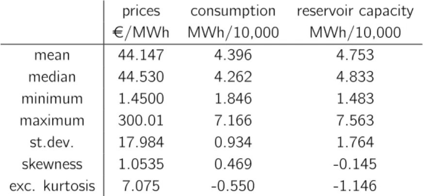
The data spans the period 1 January 2010 through 7 October 2012. We have 24,048 hourly observations that we can use from this period of time. Table 1 provides summary statistics to give an impression of the dataset that we use.
Note the high excess kurtosis of electricity prices (10.095). This is why we prefer the power function, with power decay in the tails, over an exponential form. Our interest is to estimate the parameters a0, ar, ac, ae, and α∗ in equation 4. Introducing an IID(0,1) error term, the regression equation that we apply is:
pt = ¯p−ea0+arrt+acp c t+aepet(¯s−d t) 1 1+e−α∗ +σt. (6)
whereσis the standard deviation of the error term. The model is non-linear. We apply non-linear least squares (NLS) to obtain the parameter estimates13.
12
They are available upon request.
Table 1: Summary statistics of our dataset (hourly Nord Pool day-ahead prices and consumption and weekly reservoir levels between 1 January 2010 and 7 October 2012).
prices consumption reservoir capacity
AC/MWh MWh/10,000 MWh/10,000 mean 44.147 4.396 4.753 median 44.530 4.262 4.833 minimum 1.4500 1.846 1.483 maximum 300.01 7.166 7.563 st.dev. 17.984 0.934 1.764 skewness 1.0535 0.469 -0.145 exc. kurtosis 7.075 -0.550 -1.146
The number of observations is 24,048.
4
Results
We have estimated the parameters in model 6 for the time-series of day-ahead price of each individual hour. These estimates are in table 3. But we start our discussion with estimates based on a pooled sample in order to provide insight in the fit of the model ’on average’ over the hours. We did not correct for potential individual effects, such as hourly different coefficients, which is perhaps not the econometrically best thing to do, but the estimates are consistent with the hourly estimate such we are confident that the estimates from the pooled sample provide a proper average view. Table 2 shows the parameter estimates for different (parameter) restricted versions of the regression model 6 based on a pooled sample; all 24 time series stacked. The first model is one in which we restricted the parametersar,ac,ae to be zero. That is, we restrict the supply curve to be constant. The second models allows the supply curve to depend on hydro capacity. The third model allows for hydro capacity and the prices of coal and emissions rights to structure the supply curve, i.e. the fully unrestricted model. We use scientific notation to present the very small numbers. The estimate for ar in model 2, 2.110e-03, should be read as 0.002110.
All parameter estimates in table 2 are significantly different from zero. Model 1, the constant supply curve model, explains 33% of the variation in day-ahead prices (in terms of adjusted r-squared). The estimate fora0 is 7.528 and the estimate forα∗ is -3.483, yielding anαestimate
equal to 0.030 (after applying the logit conversion). When we add the hydro capacity variable to the model, i.e. we allow that hydro capacity structures the supply curve, we observe that the adjusted r-squared increases from 33% (model 1) to 48% (model 2). The parameter estimates don’t change much. We conclude from this that adding hydro capacity strongly improves the fit of the model and that we are in favor of allowing time-variation in the supply curve to model power prices. A time-varying supply curve explains power prices better, an observation already
Table 2: NLS estimates of the parameters in the market clearing price model pt(dt) = ¯p−ea0+arrt+acpct+aepet(¯s−dt)
1
1+e−α∗ +σt.
model 1 model 2 model 3 a0 7.528 7.529 7.548
(6.260e-04) (6.066e-04) (6.478e-04) ar 2.110e-03 5.313e-04 (1.999e-05) (1.767e-05) ac -3.046e-05 (2.171e-06) ae -1.458e-03 (8.739e-06) α∗ -3.483 -3.741 -3.525 (0.012) (0.016) (0.012) α 0.030 0.023 0.029 R2 adj 0.334 0.481 0.719
The number of observations is 24,048.
Heteroskedasticity robust t-ratios are in parentheses. Scientific notation: 1e-03 = 0.001
made by Bozoianu et al. [2005], than a constant supply curve, like in Barlow [2002]. The fit of the model improves further when we add the prices of coal and emissions rights. Moving from model 2 to model 3, we observe that the adjusted r-squared increases from 48% to 72%. The market clearing price model that relates the day-ahead price to expected consumption, hydro capacity and the price of coal and emission rights explains 72% of the variation in electricity prices between January 2010 and October 2012 and from this we conclude that we can apply this model on an hourly basis to examine the relation between prices and hydro capacity while controlling for consumption and alternative production sources.
Table 3 shows the parameter estimates for each individual hour. The results for hour 1 are ob-tained from estimating the parameters using the time series of hour 1 delivery day-ahead prices and the same applies to the other 23 hours. Each time series has 1,002 observations. Our first observation is that the parameter estimates do not deviate much from those obtained from the pooled model in table 2. The estimates for the constant a0 all hover closely around 7.5, as
in the pooled sample, indicating that the pooled sample does not suffer too much from hourly differences (that we ignored in the pooled sample). Hence, we believe that the estimates from the pooled sample provide a relatively accurate ’average’ view.
We start with discussing the fit of the model for each hour. The model fits best, in terms of r-squared14, for hour 23 where it explains 80% of the variation in prices. The worst fit is for hour 9 where the model explains 55% of the variation in prices (although we still think this is a relatively high number). The reason for the difference in explanatory power becomes apparent when we compare the actual prices and fitted values graphically. Figure 1 shows the time series of actual and fitted prices for hour 9 (left) and hour 23 (right). Note the difference in the y-scale. Hour 9 exhibits several price spikes, sudden high prices, for instance around observation 50 and 750, that cannot be explained by the model even though we selected the power function model as we argued that it can better deal with fat-tails. These spikes occur as a results of short term frictions between supply and demand, something that our model cannot deal with. To deal with spikes, one would like to extend the model with some spike modeling component15, but this is outside the scope of the paper. These spikes have not occurred in hour 23 during the sample period which explains the better fit for that hour (although some deviations can be seen in the graph for hour 23 as well). The model does quite well in fitted the trend and seasonality for both; it’s the occurrence of spikes that explains the inferior fit in hour 9 compared to hour 23. As our goal is to examine the impact of hydro capacity on prices and not to examine spikes, we think that the fit of the model is sufficient to draw conclusions about the ’average’ impact of hydro capacity on day-ahead prices.
Table 3 shows that the estimates per hour are consistent in the sense that the signs of the 14
We don’t use adjusted r-squared here as we do not compare different models as we did with the pooled sample in the previous table.
15
There is a vast literature on how to do this. We refer to Huisman [2009] and Janczura and Weron [2010] among many others.
Table 3: Hourly NLS estimates of the parameters in the market clearing price model pt(dt) = ¯p−ea0+arrt+acp c t+aepet(¯s−dt) 1 1+e−α∗ +σt. hour a0 ar ac ae α∗ α R2
1 7.545 6.519e-04 -3.938e-05 -1.417e-03 -3.496 0.029 0.772
(6.065e-03) (2.060e-04) (2.188e-05) (7.920e-05) (0.115)
2 7.539 6.267e-04 -3.554e-05 -1.384e-03 -3.393 0.033 0.749
(6.186e-03) (2.209e-04) (2.262e-05) (8.505e-05) (0.101)
3 7.535 5.912e-04 -3.442e-05 -1.358e-03 -3.328 0.035 0.733
(6.232e-03) (2.339e-04) (2.312e-05) (8.952e-05) (0.104)
4 7.534 5.747e-04 -3.520e-05 -1.349e-03 -3.295 0.036 0.728
(6.202e-03) (2.378e-04) (2.356e-05) (9.329e-05) (0.101)
5 7.534 5.754e-04 -3.626e-05 -1.349e-03 -3.305 0.035 0.738
(5.969e-03) (2.306e-04) (2.344e-05) (9.323e-05) (0.097)
6 7.541 5.462e-04 -4.023e-05 -1.366e-03 -3.410 0.032 0.742
(5.406e-03) (2.074e-04) (2.263e-05) (8.640e-05) (0.094)
7 7.551 5.170e-04 -3.559e-05 -1.423e-03 -3.582 0.027 0.749
(4.566e-03) (1.868e-04) (2.197e-05) (7.913e-05) (0.087)
8 7.543 3.584e-04 -2.537e-05 -1.409e-03 -3.438 0.031 0.620
(7.119e-03) (2.019e-04) (2.511e-05) (1.092e-04) (0.120)
9 7.534 2.724e-04 -1.048e-05 -1.429e-03 -3.298 0.036 0.554
(8.905e-03) (2.222e-04) (3.003e-05) (1.306e-04) (0.130)
10 7.542 3.473e-04 -1.479e-05 -1.481e-03 -3.419 0.032 0.633
(7.249e-03) (1.984e-04) (2.710e-05) (1.113e-04) 0.118
11 7.548 4.046e-04 -1.748e-05 -1.516e-03 -3.528 0.029 0.717
(5.777e-03) (1.812e-04) (2.451e-05) (9.715e-05) 0.103
12 7.549 4.161e-04 -2.226e-05 -1.543e-03 -3.544 0.028 0.730
(5.563e-03) (1.816e-04) 2.325e-05) (9.616e-05) (0.107)
13 7.552 4.692e-04 -2.462e-05 -1.538e-03 -3.591 0.027 0.757
(5.228e-03) (1.751e-04) (2.253e-05) (8.934e-05) (0.103)
14 7.552 4.878e-04 -2.816e-05 -1.524e-03 -3.598 0.027 0.766
(5.103e-03) (1.728e-04) (2.208e-05) (8.530e-05) (0.101)
15 7.553 4.813e-04 -2.907e-05 -1.529e-03 -3.596 0.027 0.769
(4.945e-03) (1.740e-04) (2.178e-05) (8.440e-05) (0.099)
16 7.553 4.641e-04 -2.994e-05 -1.535e-03 -3.597 0.027 0.781
(4.583e-03) (1.741e-04) (2.087e-05) (8.410e-05) (0.093)
17 7.548 3.441e-04 -2.724e-05 -1.572e-03 -3.484 0.030 0.746
(4.891e-03) (1.877e-04) (2.113e-05) (9.918e-05) (0.095)
18 7.538 1.719e-04 -1.435e-05 -1.586e-03 -3.321 0.035 0.646
(7.092e-03) (2.080e-04) (2.303e-05) (1.262e-04) (0.112)
19 7.543 3.022e-04 -1.006e-05 -1.579e-03 -3.414 0.032 0.685
(6.859e-03) (1.933e-04) (2.524e-05) (1.096e-04) (0.113)
20 7.553 4.820e-04 -2.999e-05 -1.526e-03 -3.621 0.026 0.740
(5.543e-03) (1.686e-04) (2.286e-05) (9.069e-05) (0.110)
21 7.558 5.931e-04 -3.898e-05 -1.482e-03 -3.734 0.023 0.774
(4.772e-03) (1.631e-04) (2.115e-05) (8.080e-05) (0.108)
22 7.559 6.678e-04 -4.135e-05 -1.466e-03 -3.775 0.022 0.797
(4.603e-03) (1.68e-04) (2.109e-05) (7.752e-05) (0.110)
23 7.558 7.071e-04 -4.196e-05 -1.477e-03 -3.757 0.023 0.803
(4.806e-03) (1.744e-04) (2.027e-05) (7.359e-05) (0.118)
24 7.552 7.434e-04 -4.693e-05 -1.417e-03 -3.629 0.026 0.796
(5.194e-03) (1.853e-04) (2.014e-05) (7.314e-05) (0.113) The number of observations is 1,002.
Heteroskedasticity robust standard errors are in parentheses. Scientific notation: 1e-03 = 0.001
Figure 1: Actual (gray thin line) and fitted (black thick line) prices for hour 9 (left) and hour 23 (right).
0 50 100 150 200 250 300 350 0 200 400 600 800 1000 fitted actual 0 10 20 30 40 50 60 70 80 90 0 200 400 600 800 1000 fitted actual
estimates are the same for the parameters for all hours. The estimates for α range between 0.022 and 0.036 (note that the model forces α to be within 0 and 1 to obtain an increasing and convex supply curve). The signs for the prices of coal and emissions rights are all negative. This implies that an increase in these prices, increases the price of power as the exponential in the market clearing price model 4 comes with a negative sign (we explain this in more detail in the discussion about hydro capacity below).
We proceed with discussion the main topic of this paper. We question what the effect is of increasing the share of low marginal costs power production to the supply curve on the market clearing price of electricity. We examine this indirectly using data from the Nord Pool market arguing that an the marginal costs of hydro production (the value of the option to delay production) decreases when hydro capacity increases. The hypothesis that we test is therefore that an increase in hydro capacity should lead to a decrease in the day-ahead price of electricity (while correcting for consumption and prices of alternative production). Let’s focus on hour 1. The hydro capacity parameter ar estimate is 6.519e-04 (0.0006519) with standard error equal to 2.060e-04 (0.0002060). The t-statistic equals 3.165, hence we conclude that this estimate is significantly different from zero and as its sign is positive, we conclude that the estimate is significantly higher than zero. We infer from the market clearing price model 4 that a positive estimate for ar combined with the negative sign before the exponential leads to a combined negative effect between hydro capacity and power prices, therefore being in line with the hypothesis. More formally, the first order derivative of the market clearing price to hydro capacity is: d p d r =−are a0+arrt+acpct+aepet(¯s−dt) 1 1+e−α∗. (7)
As the exponential is positive and as (¯s−dt) is always positive, recall that we assumed that ¯s, the maximum supply capacity is set sufficiently higher than the maximum consumption, it becomes clear that the first order derivative in equation 7 is negative when ar is positive. Hence, we conclude for hour 1 that an increase in hydro capacity reduces the day-ahead power price. Table 3 shows that the signs of ar are positive for all hours although not always significantly different from zero. This is the case for hours 8, 9, 10, 17, 18, and 19. These are all hours in which
the fit of the model is worse due to spikes. Table 2 with the estimates from the pooled sample shows that the estimate is positive and highly significant ’on average’. Combined we conclude that an increase in hydro capacity lowers power prices and we attribute this to a reduction in the value of the option to delay production, being the marginal opportunity costs, when hydro capacity increases. An increase in hydro capacity due to increased reservoir levels is similar to adding more low marginal costs production such as wind and solar to the power supply curve. We therefore conclude that an increase in the share of wind and solar power production will lower the wholesale market price of power. We immediate note here that this result is indirect as we draw our conclusion from studying hydro capacity, but we think that it contributes to the currently limited amount of empirical results on the impact of low marginal costs renewable energy on power prices.
5
Conclusion
This paper provides indirect empirical evidence for the impact of an increased share of low marginal costs renewable power sources such as wind and solar on day-ahead power prices. With indirect we mean that we have examined this effect not directly by relating power prices to the share of renewables in a market, but indirectly through the change in the marginal costs from hydro production in the Nord Pool market. We think that this adds insight as the advantage of this method is that we can draw conclusions from a mature market whereas the alternative approach uses data from markets that change due to the increase of renewables. The disad-vantage of the method is that it is indirect, but combined with the relatively scarce empirical evidence on the impact of renewables on energy prices, we think that our results strengthens the view obtained from previous theoretical and empirical studies that an increase in the share of renewables (wind and solar) will lower the market price of power.
The second contribution of this paper is that we develop a market clearing price model by mod-eling the supply curve of power. This is done before, but not through a power function, in the sense that we allow the structure of the curve to vary over time depending on fundamentals such as hydro capacity and the prices of alternative power sources, and dealing with maximum prices which apply to all power markets that we know.
With our result, we strengthen support for the view that an increase in wind and solar supply lowers the power price. The renewable energy revolution is one in which, economically, fossil fuel power sources (positive marginal costs) have to compete with renewable power sources (low marginal costs) within the same market place. This effect strengthened with more (small scale) players entering the markets (producers with a few wind mills or solar power panels) increases competition and shifts the supply curve to the right, explaining the reduction in power prices due to an increase in renewables. Thus, an increase in sustainable energy sources with low marginal costs sources such as wind and solar will decrease power prices. This is good news for consumers, but it increases the costs of sustainable energy policies such as feed-in tariffs and at the same time lowers revenues and profits for power producers in case governments would
abandon such policies. This makes sustainable energy a less attractive investment opportunity and will lower the supply of private capital for sustainable energy investments. This effect makes the economic and policy support for renewable energy less sustainable. Policy makers have to account for this if they want to stimulate a sustainable growth of sustainable energy supply.
References
E.S. Amundsen and J.B. Mortensen. The Danish green certificate system: some simple analytical results. Energy Economics 23, 489-509, 2001.
M.T. Barlow. A diffusion model for electricity prices. Mathematical Finance, 12 (4), 287-298, 2002.
S. Borenstein. The trouble with electricity markets: understanding California’s restructuring disaster. Journal of Economic Perspectives, 16 (1), 191-211, 2002.
M. Buzoianu, A.E. Brockwell and D. Seppi. A dynamic supply-demand model for electricity prices. Carnegie Mellon University working paper, 2005.
C. Fischer. How can renewable portfolio standards lower electricity prices? RFF, discussion paper 06-20, 2006.
L. Gelabert, X. Labandeira and P. Linares. Renewable Energy and Electricity Prices in Spain.
Economics for Energy, working paper WP01, 2011
R. Huisman. An introduction to models for the energy markets. Risk Books, 2009.
D.M. Hofman and R. Huisman. Did the financial crisis lead to changes in private equity investor preferences regarding renewable energy and climate policies? Energy Policy, 47, 111-116, 2012.
R. Huisman, C.G. Koedijk, C. Kool, and F. Palm, Tail Index Estimation in Small SamplesJournal of Business and Economic Statistics, 19, 208-216, 2001.
J. Janczura and R. Weron, An empirical comparison of alternative regime-switching models for electricity spot prices. Energy Economics, 32, 1059-1073, 2010.
S.G. Jensen and K. Skytte Interactions between the power and green certificate markets.Energy Policy, 30, 425-435, 2011.
T. Jonsson, P. Pinson and H. Madsen. On the market impact of wind energy forecasts. Energy Economics, 32, 313-320, 2010.
P. Linares, F.J. Santos, M. Ventosa. Coordination of carbon reduction and renewable energy support policies. Climate Policy, 8, 377-394, 2008.
G. S´aenz de Miera, P. del Ro and I. Vizcano. Analysing the impact of renewable electricity support schemes on power prices: The case of wind electricity in Spain. Energy Policy, 36, 3345-3359, 2008.
F. Sensfuss, M. Ragwitz, and M. Genoese. The merit-order effect: A detailed analysis of the price effect of renewable electricity generation on spot market prices in Germany. Energy Policy, 36, 3076-3084, 2008.
H. Torro. Forecasting Weekly Electricity Prices at Nord Pool. Fondazione Eni Enrico Mattei, working paper, 147, 2007.
Documents de Treball de l’IEB
2011
2011/1, Oppedisano, V; Turati, G.: "What are the causes of educational inequalities and of their evolution over time in Europe? Evidence from PISA"
2011/2, Dahlberg, M; Edmark, K; Lundqvist, H.: "Ethnic diversity and preferences for redistribution " 2011/3, Canova, L.; Vaglio, A.: "Why do educated mothers matter? A model of parental help”
2011/4, Delgado, F.J.; Lago-Peñas, S.; Mayor, M.: “On the determinants of local tax rates: new evidence from Spain” 2011/5, Piolatto, A.; Schuett, F.: “A model of music piracy with popularity-dependent copying costs”
2011/6, Duch, N.; García-Estévez, J.; Parellada, M.: “Universities and regional economic growth in Spanish regions” 2011/7, Duch, N.; García-Estévez, J.: “Do universities affect firms’ location decisions? Evidence from Spain”
2011/8, Dahlberg, M.; Mörk, E.: “Is there an election cycle in public employment? Separating time effects from election year effects”
2011/9, Costas-Pérez, E.; Solé-Ollé, A.; Sorribas-Navarro, P.: “Corruption scandals, press reporting, and accountability. Evidence from Spanish mayors”
2011/10, Choi, A.; Calero, J.; Escardíbul, J.O.: “Hell to touch the sky? private tutoring and academic achievement in Korea”
2011/11, Mira Godinho, M.;Cartaxo, R.: “University patenting, licensing and technology transfer: how organizational
context and available resources determine performance”
2011/12, Duch-Brown, N.; García-Quevedo, J.; Montolio, D.: “The link between public support and private R&D effort: What is the optimal subsidy?”
2011/13, Breuillé, M.L.; Duran-Vigneron, P.; Samson, A.L.: “To assemble to resemble? A study of tax disparities among French municipalities”
2011/14, McCann, P.; Ortega-Argilés, R.: “Smart specialisation, regional growth and applications to EU cohesion policy”
2011/15, Montolio, D.; Trillas, F.: “Regulatory federalism and industrial policy in broadband telecommunications” 2011/16, Pelegrín, A.; Bolancé, C.: “Offshoring and company characteristics: some evidence from the analysis of Spanish firm data”
2011/17, Lin, C.: “Give me your wired and your highly skilled: measuring the impact of immigration policy on employers and shareholders”
2011/18, Bianchini, L.; Revelli, F.: “Green polities: urban environmental performance and government popularity” 2011/19, López Real, J.: “Family reunification or point-based immigration system? The case of the U.S. and Mexico” 2011/20, Bogliacino, F.; Piva, M.; Vivarelli, M.: “The impact of R&D on employment in Europe: a firm-level analysis” 2011/21, Tonello, M.: “Mechanisms of peer interactions between native and non-native students: rejection or integration?”
2011/22, García-Quevedo, J.; Mas-Verdú, F.; Montolio, D.: “What type of innovative firms acquire knowledge intensive services and from which suppliers?”
2011/23, Banal-Estañol, A.; Macho-Stadler, I.; Pérez-Castrillo, D.: “Research output from university-industry collaborative projects”
2011/24, Ligthart, J.E.; Van Oudheusden, P.: “In government we trust: the role of fiscal decentralization” 2011/25, Mongrain, S.; Wilson, J.D.: “Tax competition with heterogeneous capital mobility”
2011/26, Caruso, R.; Costa, J.; Ricciuti, R.: “The probability of military rule in Africa, 1970-2007” 2011/27, Solé-Ollé, A.; Viladecans-Marsal, E.: “Local spending and the housing boom”
2011/28, Simón, H.; Ramos, R.; Sanromá, E.: “Occupational mobility of immigrants in a low skilled economy. The Spanish case”
2011/29, Piolatto, A.; Trotin, G.: “Optimal tax enforcement under prospect theory”
2011/30, Montolio, D; Piolatto, A.: “Financing public education when altruistic agents have retirement concerns” 2011/31, García-Quevedo, J.; Pellegrino, G.; Vivarelli, M.: “The determinants of YICs’ R&D activity” 2011/32, Goodspeed, T.J.: “Corruption, accountability, and decentralization: theory and evidence from Mexico” 2011/33, Pedraja, F.; Cordero, J.M.: “Analysis of alternative proposals to reform the Spanish intergovernmental transfer system for municipalities”
2011/34, Jofre-Monseny, J.; Sorribas-Navarro, P.; Vázquez-Grenno, J.: “Welfare spending and ethnic heterogeneity: evidence from a massive immigration wave”
2011/35, Lyytikäinen, T.: “Tax competition among local governments: evidence from a property tax reform in Finland” 2011/36, Brülhart, M.; Schmidheiny, K.: “Estimating the Rivalness of State-Level Inward FDI”
2011/37, García-Pérez, J.I.; Hidalgo-Hidalgo, M.; Robles-Zurita, J.A.: “Does grade retention affect achievement? Some evidence from Pisa”
Documents de Treball de l’IEB
2011/39, González-Val, R.; Olmo, J.: “Growth in a cross-section of cities: location, increasing returns or random growth?”
2011/40, Anesi, V.; De Donder, P.: “Voting under the threat of secession: accommodation vs. repression” 2011/41, Di Pietro, G.; Mora, T.: “The effect of the l’Aquila earthquake on labour market outcomes”
2011/42, Brueckner, J.K.; Neumark, D.: “Beaches, sunshine, and public-sector pay: theory and evidence on amenities and rent extraction by government workers”
2011/43, Cortés, D.: “Decentralization of government and contracting with the private sector”
2011/44, Turati, G.; Montolio, D.; Piacenza, M.: “Fiscal decentralisation, private school funding, and students’ achievements. A tale from two Roman catholic countries”
2012
2012/1, Montolio, D.; Trujillo, E.: "What drives investment in telecommunications? The role of regulation, firms’ internationalization and market knowledge"
2012/2, Giesen, K.; Suedekum, J.: "The size distribution across all “cities”: a unifying approach" 2012/3, Foremny, D.; Riedel, N.: "Business taxes and the electoral cycle"
2012/4, García-Estévez, J.; Duch-Brown, N.: "Student graduation: to what extent does university expenditure matter?" 2012/5, Durán-Cabré, J.M.; Esteller-Moré, A.; Salvadori, L.: "Empirical evidence on horizontal competition in tax enforcement"
2012/6, Pickering, A.C.; Rockey, J.: "Ideology and the growth of US state government"
2012/7, Vergolini, L.; Zanini, N.: "How does aid matter? The effect of financial aid on university enrolment decisions" 2012/8, Backus, P.: "Gibrat’s law and legacy for non-profit organisations: a non-parametric analysis"
2012/9, Jofre-Monseny, J.; Marín-López, R.; Viladecans-Marsal, E.: "What underlies localization and urbanization economies? Evidence from the location of new firms"
2012/10, Mantovani, A.; Vandekerckhove, J.: "The strategic interplay between bundling and merging in complementary markets"
2012/11, Garcia-López, M.A.: "Urban spatial structure, suburbanization and transportation in Barcelona" 2012/12, Revelli, F.: "Business taxation and economic performance in hierarchical government structures"
2012/13, Arqué-Castells, P.; Mohnen, P.: "Sunk costs, extensive R&D subsidies and permanent inducement effects" 2012/14, Boffa, F.; Piolatto, A.; Ponzetto, G.: "Centralization and accountability: theory and evidence from the Clean Air Act"
2012/15, Cheshire, P.C.; Hilber, C.A.L.; Kaplanis, I.: "Land use regulation and productivity – land matters: evidence from a UK supermarket chain"
2012/16, Choi, A.; Calero, J.: "The contribution of the disabled to the attainment of the Europe 2020 strategy headline targets"
2012/17, Silva, J.I.; Vázquez-Grenno, J.: "The ins and outs of unemployment in a two-tier labor market" 2012/18, González-Val, R.; Lanaspa, L.; Sanz, F.: "New evidence on Gibrat’s law for cities"
2012/19, Vázquez-Grenno, J.: "Job search methods in times of crisis: native and immigrant strategies in Spain" 2012/20, Lessmann, C.: "Regional inequality and decentralization – an empirical analysis"
2012/21, Nuevo-Chiquero, A.: "Trends in shotgun marriages: the pill, the will or the cost?"
2012/22, Piil Damm, A.: "Neighborhood quality and labor market outcomes: evidence from quasi-random neighborhood assignment of immigrants"
2012/23, Ploeckl, F.: "Space, settlements, towns: the influence of geography and market access on settlement distribution and urbanization"
2012/24, Algan, Y.; Hémet, C.; Laitin, D.: "Diversity and local public goods: a natural experiment with exogenous residential allocation"
2012/25, Martinez, D.; Sjögren, T.: "Vertical externalities with lump-sum taxes: how much difference does unemployment make?"
2012/26, Cubel, M.; Sanchez-Pages, S.: "The effect of within-group inequality in a conflict against a unitary threat" 2012/27, Andini, M.; De Blasio, G.; Duranton, G.; Strange, W.C.: "Marshallian labor market pooling: evidence from Italy"
2012/28, Solé-Ollé, A.; Viladecans-Marsal, E.: "Do political parties matter for local land use policies?"
2012/29, Buonanno, P.; Durante, R.; Prarolo, G.; Vanin, P.: "Poor institutions, rich mines: resource curse and the origins of the Sicilian mafia"
2012/30, Anghel, B.; Cabrales, A.; Carro, J.M.: "Evaluating a bilingual education program in Spain: the impact beyond foreign language learning"
Documents de Treball de l’IEB
2012/31, Curto-Grau, M.; Solé-Ollé, A.; Sorribas-Navarro, P.: "Partisan targeting of inter-governmental transfers & state interference in local elections: evidence from Spain"
2012/32, Kappeler, A.; Solé-Ollé, A.; Stephan, A.; Välilä, T.: "Does fiscal decentralization foster regional investment in productive infrastructure?"
2012/33, Rizzo, L.; Zanardi, A.: "Single vs double ballot and party coalitions: the impact on fiscal policy. Evidence from Italy"
2012/34, Ramachandran, R.: "Language use in education and primary schooling attainment: evidence from a natural experiment in Ethiopia"
2012/35, Rothstein, J.: "Teacher quality policy when supply matters" 2012/36, Ahlfeldt, G.M.: "The hidden dimensions of urbanity"
2012/37, Mora, T.; Gil, J.; Sicras-Mainar, A.: "The influence of BMI, obesity and overweight on medical costs: a panel data approach"
2012/38, Pelegrín, A.; García-Quevedo, J.: "Which firms are involved in foreign vertical integration?"
2012/39, Agasisti, T.; Longobardi, S.: "Inequality in education: can Italian disadvantaged students close the gap? A focus on resilience in the Italian school system"
2013
2013/1, Sánchez-Vidal, M.; González-Val, R.; Viladecans-Marsal, E.: "Sequential city growth in the US: does age matter?"
2013/2, Hortas Rico, M.: "Sprawl, blight and the role of urban containment policies. Evidence from US cities"
2013/3, Lampón, J.F.; Cabanelas-Lorenzo, P-; Lago-Peñas, S.: "Why firms relocate their production overseas? The answer lies inside: corporate, logistic and technological determinants"
2013/4, Montolio, D.; Planells, S.: "Does tourism boost criminal activity? Evidence from a top touristic country" 2013/5, Garcia-López, M.A.; Holl, A.; Viladecans-Marsal, E.: "Suburbanization and highways: when the Romans, the Bourbons and the first cars still shape Spanish cities"
2013/6, Bosch, N.; Espasa, M.; Montolio, D.: "Should large Spanish municipalities be financially compensated? Costs and benefits of being a capital/central municipality"
2013/7, Escardíbul, J.O.; Mora, T.: "Teacher gender and student performance in mathematics. Evidence from Catalonia"
2013/8, Arqué-Castells, P.; Viladecans-Marsal, E.: "Banking towards development: evidence from the Spanish banking expansion plan"
2013/9, Asensio, J.; Gómez-Lobo, A.; Matas, A.: "How effective are policies to reduce gasoline consumption? Evaluating a quasi-natural experiment in Spain"
2013/10, Jofre-Monseny, J.: "The effects of unemployment benefits on migration in lagging regions"
2013/11, Segarra, A.; García-Quevedo, J.; Teruel, M.: "Financial constraints and the failure of innovation projects" 2013/12, Jerrim, J.; Choi, A.: "The mathematics skills of school children: How does England compare to the high performing East Asian jurisdictions?"
2013/13, González-Val, R.; Tirado-Fabregat, D.A.; Viladecans-Marsal, E.: "Market potential and city growth: Spain 1860-1960"
2013/14, Lundqvist, H.: "Is it worth it? On the returns to holding political office"
2013/15, Ahlfeldt, G.M.; Maennig, W.: "Homevoters vs. leasevoters: a spatial analysis of airport effects"
2013/16, Lampón, J.F.; Lago-Peñas, S.: "Factors behind international relocation and changes in production geography in the European automobile components industry"
2013/17, Guío, J.M.; Choi, A.: "Evolution of the school failure risk during the 2000 decade in Spain: analysis of Pisa results with a two-level logistic mode"
2013/18, Dahlby, B.; Rodden, J.: "A political economy model of the vertical fiscal gap and vertical fiscal imbalances in a federation"
2013/19, Acacia, F.; Cubel, M.: "Strategic voting and happiness"
2013/20, Hellerstein, J.K.; Kutzbach, M.J.; Neumark, D.: "Do labor market networks have an important spatial dimension?"
2013/21, Pellegrino, G.; Savona, M.: "Is money all? Financing versus knowledge and demand constraints to innovation" 2013/22, Lin, J.: "Regional resilience"
2013/23, Costa-Campi, M.T.; Duch-Brown, N.; García-Quevedo, J.: "R&D drivers and obstacles to innovation in the energy industry"