Tyrolean Complexity Tool: Features and Usage

Martin Avanzini

and Georg Moser

University of Innsbruck, Austria

{martin.avanzini,georg.moser}@uibk.ac.at

Abstract

The Tyrolean Complexity Tool, TCT for short, is an open source complexity analyser for term rewrite systems. Our tool TCTfeatures a majority of the known techniques for the automated characterisation of polynomial complexity of rewrite systems and can investigate derivational and runtime complexity, for full and innermost rewriting. This system description outlines features and provides a short introduction to the usage of TCT.

1998 ACM Subject Classification F.1.3 Complexity Measures and Classes, F.3.2 Semantics of Programming Languages, F.4.1 Mathematical Logic, F.4.2 Grammars and Other Rewriting Systems

Keywords and phrases program analysis, term rewriting, complexity analysis, automation

Digital Object Identifier 10.4230/LIPIcs.RTA.2013.71

1

Introduction

In order to measure the complexity of a term rewrite system (TRS for short) it is natural to look at the maximal length of derivation sequences—thederivation length—as suggested by Hofbauer and Lautemann in [13]. The resulting notion of complexity is calledderivational complexity. Hirokawa and the second author introduced in [11] a variation, calledruntime complexity, that only takes basic or constructor-based terms as start terms into account. The restriction to basic terms allows one to accurately express the complexity of a program through the runtime complexity of a TRS. An investigation into these notions is of particular interest, as both constitute aninvariant cost model for rewrite systems [7, 3], in the sense that the actual cost of a reduction on a standard model of computation, viz Turing machines, is bounded by a polynomial in the size of the start term and the length of the reduction. In particular, if the consider TRS defines a function and this TRS admits a polynomial bound on its runtime complexity, then the function is polytime computable.

As first observed in [13], it is by now folklore that termination techniques induce a certain bound on the time complexity of rewrite systems. The seminal paper by Bonfante et. al., [6] gives an early account on taming a termination technique to infer feasible, vizpolynomial, bounds. Since then, a wealth of techniques have been introduced specifically to establish polynomial complexity bounds [2, 11, 17, 18, 20, 21, 19, 15, 1, 12], see [16] for an overview. Motivated not only by these theoretical advances, but also by the annual international termination competition1_{, which features four dedicated complexity categories since 2008, a}

vast part of this theoretical body has been implemented in dedicated complexity analysers for rewrite systems. For instance, the termination proverAProVE2 features powerful support

∗ _{This work was partially supported by FWF (Austrian Science Fund) project I-603-N18.} 1

http://www.termination-portal.org/wiki/Termination_Competition/.

2

http://aprove.informatik.rwth-aachen.de/.

© Martin Avanzini and Georg Moser;

licensed under Creative Commons License CC-BY

24th International Conference on Rewriting Techniques and Applications (RTA’13). Editor: Femke van Raamsdonk; pp. 71–80

Leibniz International Proceedings in Informatics

for analysing the innermost runtime complexity of TRSs. CaT3, a variation of the very fast and powerful termination prover _TTT24_{, has excellent support to investigate derivational}

complexity, and also partial support for runtime complexity analysis. The automated complexity analyserMatchbox/Poly5verifies polynomially bounded derivational complexity. Our tool TCT, theTyrolean Complexity Tool, is an automated complexity analyser for TRSs in the line of the aforementioned tools. Its distinct feature is that it is currently the only tool that is competitive, and provides dedicated techniques, for both runtime and derivational complexity analysis. TCT isopen-source, released under theGNU Lesser General Public License (LGPL) Version 3, and available from

http://cl-informatik.uibk.ac.at/software/tct/.

The theoretical framework underlyingTCT, which allows for this generality and modularity, is documented in separate work [5]. Here we want to outline the practical aspects ofTCT, version 2.0 to be precise. In Section 2 we provide a brief description of the implementation including accompanying libraries. Section 3, where we discuss features and usage of our tool, constitutes the main part of this work. In Section 4 we indicate future work and conclude.

2

Implementation

Our tool is implemented in the strongly typed, lazy functional programming language

Haskell6and compiles on theGlasgow Haskell CompileronGNU Linux. The sources consist of about 13,000 lines of code, and additionally 4,000 lines of documentation. Out of the 73 modules, 43 modules are dedicated to the implementation of the various techniques (roughly 56 % of the code), the remaining modules provide the core of TCTand utilities. Our tool makes also use of followingHaskelllibraries, separately available from theTCThomepage7_,

that have been specifically developed forTCT.

qlogicprovides facilities for dealing with propositional logic, and consists of approxim-ately 3100 lines of code. Notably it defines an interface to SAT-solvers, including routines to efficiently translate Boolean formulas to conjunctive normal form. Also it features support for theories over natural numbers and integers, implemented bybit-blasting.

termlibprovides term rewriting functionality, and consists of around 2100 lines of code.

parfold is a small library that provides folding capabilities over lists of concurrently evaluated monad actions, a simple but convenient abstraction to concurrent programming.

3

Features and Usage

The Tyrolean Complexity Tool currently features 23 techniques which are available for runtime and, where applicable, for derivational complexity analysis. Our implementation follows closely the framework provided in [5] which ensures that the techniques are implemented in a modular way. We indicate some characteristic methods implemented inTCT:

Matrix Interpretations: Our tool features an implementation ofmatrix interpretations over the naturals [8], as well asarctic interpretations[14]. To weaken monotonicity requirements

3 _{Available from} http://cl-informatik.uibk.ac.at/software/cat/. 4 _{Available from} http://cl-informatik.uibk.ac.at/software/ttt2/. 5 _{Available from} http://dfa.imn.htwk-leipzig.de/matchbox/poly/.

6 _{An open-source product of more than twenty years of cutting-edge research, c.f. http://haskell.org/.} 7

we have integrated theusable arguments criterion[12] and usable rules w.r.t. argument filterings [10]. In order to give polynomial bounds on the induced complexity,TCT can employtriangular matrices [18], or use the criterions defined in [15, 20]. Moreover, our implementation also integrates theweight gap principle [12].

Polynomial Path Orders: Up to our knowledge,TCT is the only tool that features an im-plementation of polynomial path orders[2, 4] as well as the recently introduced small polynomial path orders [1]. Both orders constitute a miniaturisation of recursive path orders that induce polynomially bounded innermost runtime complexity. Whereas the former order can only deduce if the innermost runtime complexity is in principle polyno-mial, its small brother allows a precise control on the complexity certificate obtained.

Match-Bounds: Match-Boundsfor term rewrite systems [9] is a powerful termination method that induces linear complexity. Our tool supports match-,top- androof-bounds both for derivational, and its refinement to runtime complexity analysis.

Weak Dependency Pairs and Dependency Tuples: The introduction ofweak dependency pairs greatly simplifies the task of estimating the runtime complexity of TRSs. Our tool supports this method as well as its refinement to innermost rewriting, calleddependency tuples in [19]. This technique gives rise to advanced techniques specifically designed for the dependency pair setting, notably various simplifications,usable rules,path analysis, (safe) reduction pairs as well asdependency graph decomposition, compare [12, 19, 5]. In the following, we discuss usage of TCT.

3.1

Web Interface

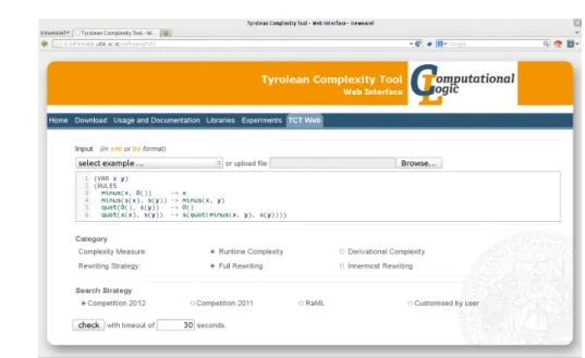
Figure 1Web Interface of TCT.

Our web interface, accessible from the TCT homepage, provides a convenient way to useTCTwithout the necessity to install the software. The interface is aimed for simplicity, compare Figure 1. For the curious user that wants to play around withTCT, we also provide a wealth of interesting examples. The web interface is configured so that by default an upper bound on theruntime complexity of the given rewrite system is estimated. This behaviour can be modified undercategory, where the user can pick from the four different complexity measuresTCTcurrently supports. On success this certificate is presented to the user, together with a proof script that explains in considerable detail how the certificate was obtained.

To find a proof in a reasonable amount of time, the different techniques implemented in

TCTneed to be combined wisely. This combination depends on the one hand on the input problem, but on the other hand also on the available hardware. InTCT,proof search is not hard-wired, instead it is guided by a(proof) search strategy. The interface allows to specify such a search strategy from a set of pre-defined proof search strategies. Besides the search strategies employed in recent competitions, the web-interface currently offers the search strategyRaML, specifically designed for functional programs given as rewrite systems, and a customisable search strategy that allows the explicit inclusion/exclusion of methods.

3.2

Command-Line Interface

The full power of TCT is available through its command-line interface. For installation instructions we refer the reader to the homepage. Here we want to briefly outline usage and customisation, comprehensive documentation can be found online. TCTis run by

$ tct [options] [-s <strategy>] <file>,

from the command-line, where[options]specify an optional list of command-line options,

<strategy>specifies optionally a proof search strategy, and<file>theinput file. The input file must adhere either the oldTPDB format8 or the newXTC Format9.

A list of options can be obtained by typingtct --help. In the command-line interface, the proof search strategy is given as anS-expression of the form

(<name> [:<argname> <arg>]* _[<arg>]*_),

where outermost parentheses can be dropped. Here <name>refers to the name of a proof technique, also calledprocessor, the list[:<argname> <arg>]*can be used to specifynamed optional arguments, and the list [<arg>]* gives a possibly empty sequence ofpositional arguments. As an example,

fastest (timeout 3 (bounds :enrichment match)) (matrix :degree 2),

provides a valid proof search strategy inTCT. Herefastestis used to combine one or more processors in parallel, in this case theboundandmatrixprocessors, solving the input problem with whichever processor succeeds first. The defined search strategy advisesTCTto check for three seconds formatch-boundedness of the input problem, respectively compatibility with a matrix interpretation that induces a quadratic upper bound. All implemented techniques, including a wealth ofprocessor combinatorslikefastestandtimeout, can be applied directly from the command-line with the option-s <strategy>. A complete list of available search strategies, including synopsis and documentation, can be obtained by typingtct --list.

Besides basic options given on the command-line,TCTcan be configured by modifying theconfiguration file, which resides in~/.tct/tct.hs by default. ThisHaskellsource-file defines the actual binary that is run each timeTCTis called. Thus the full expressiveness of Haskell is available; as a downside, it requires also a working Haskell environment. A minimal configuration is generated automatically on the first run of TCT. This initial configuration consists of a set of convenient imports and the IO actionmain together with a configuration recordconfig. The configuration record passed inmainallows one to overwrite various flags of TCT. Most importantly, through the field strategies it also allows the modification of the list of proof search strategies that can be employed.

8

http://www.lri.fr/~marche/tpdb/format.html.

9

import Tct (tct) import Tct.Instances $... main :: IO () main = tct config config :: Config

config = defaultConfig { strategies = strategies }where

strategies = [ matrices ::: strategy "matrices" ( optional naturalArg"start" (Nat 1) :+: naturalArg ) , withDP ::: strategy "withDP" ]

matrices (Nats :+: Natn) =

fastest [ matrix ‘withDimension‘d ‘withBits‘ bitsForDimension d|d <- [s..s+n] ]where

bitsForDimensiond = if d < 3 then 2 else 1 withDP =

(timeout 5 dps <> dts)

>>> try (exhaustively partitionIndependent) >>> try cleanTail

>>> try usableRuleswhere

dps = dependencyPairs >>> try usableRules >>> wgOnUsable dts = dependencyTuples

wgOnUsable = weightgap ‘withDimension‘ 1 ‘wgOn‘ WgOnTrs

Figure 2Configuration defining two new search strategies, calledmatricesandwithDP.

In Figure 2 we depict a modified configuration that defines two new search strategies, calledmatricesandwithDP. Strategies are added by overwriting the field strategieswith a list of declarations of the form

<code> ::: strategy "<name>" [<parameters-declaration>] .

Here<code>refers to a definition that evaluates to a processor, and"<name>"as well as the optional parameters-declaration specify how this code is accessible from the command-line. For instance, the first declaration in Figure 2 defines a new search strategy namedmatrices, which is available by supplying the option-s "matrices [:start <nat>] <nat>"to the

TCTexecutable. Here the parameters tomatricesare declared by

optional naturalArg "start" (Nat 1) :+: naturalArg ,

where the infix operator:+: is used to specify sequences of parameters. As indicated by the constructornaturalArg, the search strategymatricesexpect twonatural numbers as arguments. In contrast to the second parameter, the first is optional and defaults to the natural number1.

In Figure 2, these parameters are provided to the code ofmatrices. Using parameterss andnas supplied on the command-line, the code evaluates to a processor that searches for ncompatible matrix interpretations of increasing dimension, in parallel. Bothmatrixand

fastest, along with other processors, combinators andmodifierslikewithDimensionand

withBits, are exported by the moduleTct.Instances.

The second proof search strategy declared in Figure 2 defines a transformationcalled

withDP. Transformations are a specific class of processors, that generate from the given input problem a possibly empty set ofsub-problems, in a complexity-preserving manner.10

For every transformationt and processor p, one can use theprocessor t >>| pwhich first applies transformationtand then solves the resulting sub-problems usingp.Search strategy declarations perform such a lifting of transformation implicitly, the declaration ofwithDP

for instance results in a search strategy available as withDP <processor>. Besides the

10_{Transformations were introduced in Version 1.7 of}

TCT. Although any processor likematrixcould also be defined as a transformation, the distinction inTCTis present mainly for historical reasons.

combinator>>|and its variation>>||, where the given processor pis applied in parallel on all sub-problems, the moduleTct.Instancesprovides a wealth of transformation combinators. We briefly discuss here the most important ones. The transformationt1 <> t2 employed in

withDPfirst applies transformationt1, only if this is unsuccessful it applies transformationt2

on the input problem instead. A variation of the combinator is given byt1 <||> t2that applies

transformationst1andt2in parallel, resulting in the sub-problems of whichever transformation

succeeds first. The combinator<||>thus implements a form of non-deterministic choice. The combinator>>> defines composition of transformations, in the sense that the transformation t1 >>> t2 first applies transformation t1 and then transformation t2 on all resulting

sub-problems. We remark that any transformation aborts if it is inapplicable. The combinator

tryoverrides this behaviour, in the sense thattry t behaves exactly liket shouldt succeed, otherwise it behaves as an identity. Finally, the combinator exhaustively, defined by

exhaustively t = t >>> try (exhaustively t), appliest in an iterated fashion.

In total, the defined search strategywithDPdepicted in Figure 2 applies weak dependency pairs (as realised in the definition ofdps), or dependency tuples (as realised bydts) should the former fail. This transformation is followed by a sequence of syntactic simplifications, if applicable. We remark the thoughtful use oftry. The transformationdpsfails if theweight gap principle cannot be established on all TRS rules, i.e., rules that are not dependency pairs. The latter is implemented by the transformationwgOnUsable, and constitutes an implementation of [12, Theorem 6.5]. We finally point out that an extended version of the transformationwithDPis available in TCTas toDP.

3.3

Interactive Interface

TCTfeatures also aninteractive interface,TCT-ifor short. In this section we guide the reader through a small interactive session that outlines the main features, elaborate documentation of this mode is again provided online.

Thissemi-automatic mode is in particular useful when investigating into tight(er) com-plexity bounds, and to crack hard-to-solve problems. The interactive interface constitutes essentially of a tiny wrapper aroundghci, the interpreter bundled with theGlasgow Haskell compiler. Users familiar with ghci will note that all features available in ghci are also available inTCT-i. The interactive interface is started from the command-line by supplying the option-ito theTCTexecutable.

$tct -i

GHCi, version 7.4.1: http://www.haskell.org/ghc/ :? for help

$...

This is version 2.0 of the Tyrolean Complexity Tool.

(c) Martin Avanzini <[email protected]>, Georg Moser <[email protected]>, and Andreas Schnabl <[email protected]>.

This software is licensed under the GNU Lesser General Public License, see <http://www.gnu.org/licenses/>.

Don’t know how to start? Type ’help’. TCT>

The interactive interface maintains a proof state, which consists conceptually of a list of open problemstogether with proof information. The commandload "<file>" is used to populate the proof state by the TRS given as argument.

TCT> load "examples/div.trs"

---Selected Open Problems: ---Strict Trs: { -(x, 0()) -> x , -(s(x), s(y)) -> -(x, y) , %(0(), s(y)) -> 0()

, %(s(x), s(y)) -> s(%(-(x, y), s(y))) } StartTerms: basic terms

Strategy: none

---The current state can be inspected at any time by typing the commandstate. We note that the rewrite strategy and set of start terms are defined in accordance to the input file. The commandsset[DC|RC|IDC|IRC]provide short-hands to these accordingly.

The primary means to modify the proof state is the use of the command apply. This command takes a single argument, a transformation or processor respectively, which is applied by default on all open problems collected in the current proof state. Both processors and transformations as imported fromTct.Instancesqualify as arguments toapply. Of course one can also use the various combinators that we have seen so far to construct more complex arguments. Notably, sinceTCT-iloads the configuration file of TCT, all declarations given in the configuration are available as top-level bindings, and can thus be used in conjuction with

apply. Recall that our configuration defines a transformationwithDPthat computes weak dependency pairs or dependency tuples respectively, applying various transformations on success. We use this transformation to simplify the input problem.

TCT> apply withDP

Problems simplified. Use ’state’ to see the current proof state.

The output ofapplyis intentionally kept short.11 By typingstate one can observe that our initially loaded complexity problem has been replaced by the problem obtained by our transformationwithDP. To see that proof generated so far, one can use the commandproof. Note that as long as the list of open problems is not empty, this proof is marked as open.

TCT> proof

1) dp [OPEN]:

---We consider the following problem: Strict Trs:

{ -(x, 0()) -> x

, -(s(x), s(y)) -> -(x, y) , %(0(), s(y)) -> 0()

, %(s(x), s(y)) -> s(%(-(x, y), s(y))) } StartTerms: basic terms

Strategy: none

We add following weak dependency pairs:

$...

1.1) Open Problem [OPEN]:

---We consider the following problem: Strict DPs:

{ -^#(x, 0()) -> c_1(x)

, -^#(s(x), s(y)) -> c_2(-^#(x, y))

, %^#(s(x), s(y)) -> c_4(%^#(-(x, y), s(y))) } Weak Trs:

{ -(x, 0()) -> x

, -(s(x), s(y)) -> -(x, y) } StartTerms: basic terms Strategy: none

11_{To override this behaviour and see actions performed, one can use the command}

setShowProofs, or

alternatively set the fieldinteractiveShowProofstoTruein the configuration record of TCT.

Besidesstateandproof, following commands allow for further inspection of the current proof state. The command problemsreturns the list of open problems, wdgs and cwdgs

return the corresponding dependency graphs respectively congruence graph anduargsreturns the usable argument positions. Cf. [12] for an explanation of these attributes. For instance, we can usecwdgsto inspect the congruence graph of our open problem as follows.

TCT> [cwdg] <- cwdgs

Congruence Graph of Problem 1: ->1:{1,2}

| ‘->2:{3}

Here dependency-pairs are as follows:

Strict DPs:

{ 1: -^#(x, 0()) -> c_1(x)

, 2: -^#(s(x), s(y)) -> c_2(-^#(x, y))

, 3: %^#(s(x), s(y)) -> c_4(%^#(-(x, y), s(y))) } TCT> :module +Tct.Method.DP.DependencyGraph

TCT> isEdgeTo cwdg 1 2

True

Once the list of open problem is empty, the complexity of the input problem has been successfully proven. We can do so on our running example using the matrix processor that we have already used before.

TCT> apply matrix

Hurray, the problem was solved with certicficate YES(O(1),O(n^2)). Use ’proof’ to show the complete proof.

We have found a closed proof that verifies that our initial problem has at most quadratic runtime complexity. We remark that the runtime complexity of the input TRS is even linear. Inspecting the proof we see that the imprecision in the certificate was introduced in the last proof step. FortunatelyTCT-iprovides a commandundothat can be used to revert the effect ofapply. In fact, it reverts any modification on the proof state, except of course the effect ofundo itself. We refine the proof by restricting theinduced degree of the constructed interpretation.

TCT> undo

Current Proof State

---Selected Open Problems:

---Strict DPs:

{ -^#(x, 0()) -> c_1(x)

, -^#(s(x), s(y)) -> c_2(-^#(x, y))

, %^#(s(x), s(y)) -> c_4(%^#(-(x, y), s(y))) } Weak Trs:

{ -(x, 0()) -> x

, -(s(x), s(y)) -> -(x, y) } StartTerms: basic terms Strategy: none

---TCT> apply$ matrix ‘withDegree‘ Just 1

Hurray, the problem was solved with certicficate YES(O(1),O(n^1)). Use ’proof’ to show the complete proof.

Here the functionwithDegreeis used to modify the default parameters as defined inmatrix.12

We finally end up with a closed proof that verifies that our loaded TRS has linear runtime complexity. Using the commandwriteProof "<file>" one can write the constructed proof to the given file.

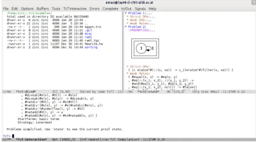
This completes the short tutorial. We remark that for the GNU Emacs13 enthusiast, we have also crafted a small major-mode forTCT-i. This mode is available in the source distribution ofTCT. The mode can be started by typingM-x tctintoGNU Emacs. In addition to the features explained above, the major-mode provides a refurbished view on the proof state, compare Figure 3 which shows an example session. The approximated dependency graph depicted in Figure 3 is visualised using thedottool of the Graphviztoolkit.14

Figure 3TCTMajor Mode forGNU Emacs.

4

Conclusion and Future Work

Our complexity analyser TCT has matured to a state where we can say that it is both versatile and powerful. This is underpinned by the experimental evidence given online15 which highlights in particular the strength of the underlying combination framework presented in [5].

We of course seek to keep the implementation in line with the active research community. In the upcoming version, we also intend to remove some out-dated design choices, foremost the separation of processors and transformations, which will result in a significantly simplified core. Also, we currently investigate the integration of constrained rewriting. This should leverage the design of complexity preserving reductions fromreal world programs to rewrite systems, in the hope thatTCTwill act as a powerful backend.

Acknowledgement

Foremostly we thank Andreas Schnabl for his major role in the development ofTCT. Moreover, we thank Martin Korp, Christian Sternagel, and Harald Zankl as (former) members of the_TTT2 team for ongoing discussions. We also thank Bertram Felgenhauer for valuable discussions concerning the implementation. Finally, we also thank the anonymous reviewers for valuable suggestions that improved the presentation of this paper.

13

GNU Emacsis open-source and available fromhttp://www.gnu.org/s/emacs/.

14_{The toolkit is open-source and available from}

http://www.graphviz.org/.

15_C.f.

http://cl-informatik.uibk.ac.at/software/tct/experiments/tct2/.

References

1 M. Avanzini, N. Eguchi, and G. Moser. New Order-theoretic Characterisation of the Poly-time Computable Functions. In Proceedings of the 10th Asian Symposium Programming Languages and Systems, number 7705 in LNCS, pages 280–295. Springer, 2012.

2 M. Avanzini and G. Moser. Complexity Analysis by Rewriting. InProc. of 8th FLOPS, volume 4989 of LNCS, pages 130–146. Springer, 2008.

3 M. Avanzini and G. Moser. Closing the Gap Between Runtime Complexity and Polytime Computability. InProc. of 21st RTA, volume 6 ofLIPIcs, pages 33–48, 2010.

4 M. Avanzini and G. Moser. Polynomial Path Orders: A Maximal Model. 2012. Submitted to LMCS. Technical Report available athttp://arxiv.org/abs/1209.3793.

5 M. Avanzini and G. Moser. A Combination Framework for Complexity. InProc. of 24th RTA. LIPIcs, 2013. Technical Report available athttp://arxiv.org/abs/1302.0973.

6 G. Bonfante, A. Cichon, J.-Y. Marion, and H. Touzet. Algorithms with Polynomial Inter-pretation Termination Proof. JFP, 11(1):33–53, 2001.

7 U. Dal Lago and S. Martini. Derivational Complexity is an Invariant Cost Model. InProc. of 1st FOPARA, 2009.

8 J. Endrullis, J. Waldmann, and H. Zantema. Matrix Interpretations for Proving Termina-tion of Term Rewriting. JAR, 40(2-3):195–220, 2008.

9 A. Geser, D. Hofbauer, J. Waldmann, and H. Zantema. On Tree Automata that Certify Termination of Left-Linear Term Rewriting Systems. In Proc. of 16th _{RTA, number 3467}

in LNCS, pages 353–367. Springer, 2005.

10 J. Giesl, R. Thiemann, P. Schneider-Kamp, and S. Falke. Mechanizing and Improving Dependency Pairs. JAR, 37(3):155–203, 2006.

11 N. Hirokawa and G. Moser. Automated Complexity Analysis Based on the Dependency Pair Method. InProc. of 4th IJCAR, volume 5195 ofLNAI, pages 364–380, 2008.

12 N. Hirokawa and G. Moser. Automated Complexity Analysis Based on the Dependency Pair Method. 2012. Submitted to IC, available athttp://arxiv.org/abs/1102.3129.

13 D. Hofbauer and C. Lautemann. Termination Proofs and the Length of Derivations. In Proc. of 3rd _{RTA, volume 355 ofLNCS, pages 167–177. Springer, 1989.}

14 A. Koprowski and J. Waldmann. Max/Plus Tree Automata for Termination of Term Re-writing. AC, 19(2):357–392, 2009.

15 A. Middeldorp, G. Moser, F. Neurauter, J. Waldmann, and H. Zankl. Joint Spectral Radius Theory for Automated Complexity Analysis of Rewrite Systems. InProc. of 4th CAI, volume 6742 ofLNCS, pages 1–20. Springer, 2011.

16 G. Moser. Proof Theory at Work: Complexity Analysis of Term Rewrite Systems. CoRR, abs/0907.5527, 2009. Habilitation Thesis.

17 G. Moser and A. Schnabl. Proving Quadratic Derivational Complexities using Context Dependent Interpretations. In Proc. of 19th _{RTA, volume 5117 ofLNCS, pages 276–290.}

Springer, 2008.

18 G. Moser, A. Schnabl, and J. Waldmann. Complexity Analysis of Term Rewriting Based on Matrix and Context Dependent Interpretations. InProc. of 28th _{FSTTCS, LIPIcs, pages}

304–315, 2008.

19 L. Noschinski, F. Emmes, and J. Giesl. A Dependency Pair Framework for Innermost Complexity Analysis of Term Rewrite Systems. In Proc. of 23rd _{CADE, LNAI, pages}

422–438. Springer, 2011.

20 J. Waldmann. Polynomially Bounded Matrix Interpretations. In Proc. of 21st RTA, volume 6 ofLIPIcs, pages 357–372, 2010.

21 H. Zankl and M. Korp. Modular Complexity Analysis via Relative Complexity. InProc. of 21st RTA, volume 6 ofLIPIcs, pages 385–400, 2010.