Data-Driven Appointment Scheduling

UC Berkeley Electronic Theses and Dissertations

Data-Driven Appointment Scheduling

Permalink https://escholarship.org/uc/item/8bt4012r Author Gurek, Tugce Publication Date 2019 Peer reviewed|Thesis/dissertation

eScholarship.org Powered by the California Digital Library University of California

by Tugce Gurek

A dissertation submitted in partial satisfaction of the requirements for the degree of

Doctor of Philosophy in

Engineering - Industrial Engineering and Operations Research in the

Graduate Division of the

University of California, Berkeley

Committee in charge:

Professor Philip M Kaminsky, Chair Professor Rhonda Righter

Professor Anil Aswani Professor Haiyan Huang

Copyright 2019 by Tugce Gurek

Abstract

Data Driven Appointment Scheduling by

Tugce Gurek

Doctor of Philosophy in Engineering - Industrial Engineering and Operations Research University of California, Berkeley

Professor Philip Kaminsky, Chair

Advances in electronic medical records and healthcare databases enable researchers to easily acquire and analyze large amounts of data, and to build data-driven models to improve the system performance. Surgical departments, in particular, utilize a variety of expensive resources, so efficient appointment scheduling and sequencing decisions that minimize patient-surgeon waiting time and the patient-surgeon-operating room idle time substantially reduce costs. We aim to improve the way that schedules are generated by incorporating both dynamically updated data sets, and the opinions of surgeons.

Our research focuses on appointment scheduling of stochastic tasks on a single server where the task durations are challenging to estimate. The task types are known prior to the appointment date but the task duration data is initially limited so that the estimates need to be continuously updated. Appointment scheduling involves both sequencing the tasks and setting the start time of those tasks. Our goal is to develop a data driven appointment scheduling algorithm for sequencing and scheduling tasks. Our research is motivated by a project we have completed with University of California, San Francisco (UCSF) on surgical scheduling where the tasks are the surgical procedures and the server is the operating room.

In Chapter 1 we introduce the appointment scheduling problem with a motivating example of surgical appointment scheduling. We run some simulations to show patient-surgeon waiting time (tardiness) and the surgeon-operating room idle time (earliness) can be reduced by changing the sequence of the procedures and the start times of the procedures. We go over the appointment scheduling literature with various objective functions. We analyze the objective of minimizing expected earliness and tardiness and bound the performance of the commonly used sequencing heuristic based on the standard deviation of procedure duration.

In Chapter 2 we focus on data-driven appointment scheduling. Without making any dis-tributional assumptions we use the empirical distributions of the procedures while computing the objective function which is the expectation of weighted earliness and tardiness. We study the continuity and the convexity of the objective function and the conditions under which there is an integral optimal solution. We briefly go over the methods to optimize the objective function and also constrain the search space containing the minimizer. We develop sequencing heuristics tailored for this problem. Lastly, we consider data selection algorithms

when there are categorical features such as name of the surgeon or surgeon estimates about how long the next procedure might take.

Contents

1.1.2 Analysis of Existing Data . . . 2

1.1.3 Simulation Study of Alternative Sequencing Rules . . . 3

1.2 Literature Review . . . 5

1.2.1 Appointment Scheduling: Minimizing Expected Earliness and Tardiness 5 1.2.2 Alternative Objective Functions of Appointment Scheduling . . . 10

1.2.3 Data-Driven Newsvendor Problems . . . 11

1.3 Model and Preliminary Results . . . 12

1.3.1 Notation . . . 12

1.3.2 Minimizing Expected Earliness and Tardiness with Known Distributions 13 1.3.3 Minimizing Expected Earliness and Tardiness using the Empirical Distribution . . . 16

1.3.4 Performance Bound of the Sequencing Heuristic Based on the Standard Deviation of Procedure Duration . . . 19

1.3.5 Worst Case Given the Variance . . . 30

2 Data-Driven Appointment Scheduling 34 2.1 Properties of the Objective Function . . . 34

2.2 Computation of the Optimizer . . . 40

2.2.1 Smoothing the Objective Funtion . . . 41

2.3 Online Algorithm . . . 45

2.3.1 New Notation . . . 45

2.3.2 Search Space . . . 46

2.3.4 Motivating Questions and Answers . . . 53

2.3.5 Sequencing . . . 56

2.4 Data Selection . . . 69

2.4.1 Expert (Surgeon) Opinions . . . 70

2.4.2 Feature Selection . . . 73

3 Conclusion 77

List of Figures

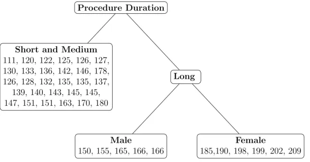
1.1 Results of the simulation runs . . . 4 1.2 Average earliness and tardiness . . . 4 1.3 Network representation of the appointment scheduling problem given the sequence 9 2.1 Computational Comparison of the Sequencing Heuristics . . . 68 2.2 Computational Comparison of the Sequencing Heuristics . . . 68 2.3 Decision tree built using the feature selection algorithm using the data set 1. . . 75 2.4 Decision tree built using the feature selection algorithm using the data set 2. . . 76

List of Tables

2.1 Complexity of evaluating the objective function value at an integer schedule assuming the procedure duration data has only integer entries (Begen, 2010). . . 39 2.2 Complexity of evaluating the objective function value at any schedule with

Acknowledgments

First and foremost, I would like to express my sincere gratitude and appreciation to my advisor, Professor Philip M. Kaminsky for his guidance, optimism and for believing in me. I really appreciate him making time to discuss our research, to go further and overcome challenges. His dedication to his work and enthusiasm about his research have inspired me all the time. I am grateful to Professor Rhonda Righter, Professor Anil Aswani, and Professor Haiyan Huang for their academic guidance and being on my qualifying exam and dissertation committee. I would like to thank my committee members for their valuable feedback during my graduate studies.

I would like to thank the IEOR the department staff, especially Keith McAleer, Anayancy Paz, Sonia Chahal, Rebecca R. Pauling, Yeri Caesar-Kaptoech, Diana Salazar and Heather Iwata. I appreciate their timely help.

I am grateful to Kamil Nar and Orhan Ocal who have given me an unconditional support and valuable advice through my PhD journey. I am incredibly proud of being in the research group with Heejung Kim, Shiman Ding, Arman Jabbari, Stewart Liu, Yang Wang and Dan Bu. I am also happy that our paths crossed with Kevin Li, Quico Spaen, Rebecca Sarto, Birce Tezel, Auyon Siddiq, Jiaying Shi, Mo Zhou, Jiung Lee, Erik Bertelli, Guang Yang, Amber Richter, Cheng Lyu, Angel Yang, Wen Gao, Jared Bauman, Carlos Deck, Brent Eldridge, Alfonso Lobos, Salar Fattahi, Mark Velednitsky, and Renyuan Xu. I am thankful to Sevi Baltaoglu for being a wonderful companion, Aydan Inak and Burak Onal for our weekly motivating phone calls, Dilara Semerci and Regis Frey for being a part of Berkeley team.

I appreciate my family’s unconditional support from Turkey. I thank my parents for taking time out of their busy schedules to visit me frequently. My cousins, uncles, aunts, even my grandmother take long-haul flight just to spend time with me. I am grateful that I am part of this loving, caring family: Aysel, Cemal, Atilla, Ayse Gul, Bahadir, Faliha, Dorukan, Bengihan, Cenk, Yasemin, Selin, Alp Gurek, Aynur, Metin Mete, Idil Topcuoglu, Nezahat, Ahmet, Cagatay, Muge, Cagan Kanal, Gozde, Evren, Eren Ege, Melissa Kayakiran. Last but not least, I would like to thank my husband Mehmet Mustafa Yilmaz for making my life filled with so much happiness and love.

Chapter 1

Appointment Scheduling

1.1

Introduction

This research focuses on appointment scheduling of stochastic tasks on a single server where the task processing durations are challenging to estimate. Appointment scheduling involves both sequencing tasks, and setting estimated start times of those tasks. Tasks types are known prior to the appointment date, but task duration data is initially limited so duration estimates are continuously updated. Our goal is to develop a data-driven approach to sequencing and scheduling these tasks that also integrates expert knowledge into the scheduling decision.

Our work is motivated by a project we completed with UCSF on surgical scheduling, where the tasks are surgeries and the server is the operating room. Advances in electronic medical records and healthcare databases enable researchers to easily acquire and analyze large amounts of data, and to build data-driven models to improve the system performance. Surgical departments, in particular, utilize a variety of expensive resources, so efficient appointment scheduling and sequencing decisions that minimize patient-surgeon waiting time and the surgeon-operating room idle time substantially reduce costs. Our eventual goal is to improve the way schedules are generated by incorporating both dynamically updated data sets, and the opinions of surgeons.

In Chapter 1 we introduce the appointment scheduling problem with a motivating example of surgical appointment scheduling. We run some simulations to show patient-surgeon waiting time (tardiness) and the surgeon-operating room idle time (earliness) can be reduced by changing the sequence of the procedures and the start times of the procedures. We go over the appointment scheduling literature with various objective functions. We analyze the objective of minimizing expected earliness and tardiness and bound the performance of the commonly used sequencing heuristic based on the standard deviation of procedure duration.

In Chapter 2 we focus on data-driven appointment scheduling. Without making any dis-tributional assumptions we use the empirical distributions of the procedures while computing the objective function which is the expectation of weighted earliness and tardiness. We study the continuity and the convexity of the objective function and the conditions under which

there is an integral optimal solution. We briefly go over the methods to optimize the objective function and also constrain the search space containing the minimizer. We develop sequencing heuristics tailored for this problem. Lastly we talk about data selection algorithms if there are categorical features such as name of the surgeon or surgeon estimates about how long the next procedure might take.

1.1.1

Motivation

Caring WiselyTM _{is a program run by University of California, San Francisco (UCSF) Center}

for Healthcare Value. This program is designed to fund interventions that can reduce costs, improve value and enable innovation. We collaborated with Lindsay Hampson, MD, Max Meng, MD and their team on Operating Wisely: Operating Room Teamwork in Improving and Measuring Efficiency (ORTIME), a Caring WiselyTM _project.

The ORTIME project focused on increasing operating room (OR) efficiency without increasing the preoperative, intraoperative, and postoperative complication rates. OR efficiency is defined in terms of the percentage of on-time cases, patient-surgeon waiting time, surgeon-operating room idle time and non-operative OR time. Improving OR efficiency requires improving prediction of procedure times (schedules) while:

1. Increasing the percentage of on-time cases,

2. Reducing patient-surgeon waiting time, surgeon-operating room idle time, and 3. Minimizing non-operative OR time (e.g. turnover time).

Operating rooms account for a substantial amount of revenue and hospital expenses. Non-operative OR time does not generate revenue, so the goal is to minimize or eliminate it if possible. Turning over a room is a non-operative OR time which requires surgeons, anesthesiologists, nurses and other staff to work together. OR turnover time is the time between when a patient leaves an OR after a procedure and the time the next patient arrives in the OR for the next procedure. Decreasing turnover time increases OR efficiency.

Data about current operations has been collected for several years. We analyzed this data to determine the current scheduling efficiency, and used this data combined with a simulation to assess the impact of alternative sequencing rules and appointment scheduling approaches.

1.1.2

Analysis of Existing Data

The baseline data we obtained from UCSF Medical Center at Mt. Zion shows that 8.6% of cases are completed before the scheduled end time and only 13.5% are completed within 15 minutes of the scheduled end time. This data consists of the information about 14593 different cases (note that confidential data was encoded to hide confidential information). The data includes:

• Timeline of the procedures (Surgery date, Time patient enters and exits OR, Time procedure starts and ends, Scheduled start time and end time)

• Procedure type and code

Actual duration of the procedure (time spent in the room), which is the difference between the time patient enters the OR and exits, can be directly obtained using the baseline data. Unfortunately the data doesn’t have the actual turnover time after procedure. So we approximated the turnover time as (upper bound on the actual turnover time):

P roc Duration[i] =T ime Exit OR[i]−T ime Enter OR[i]

T urnover[i] =       

T ime Enter OR[i+ 1]−T ime Exit OR[i]

if Sched Start T ime[i+ 1] =Sched End T ime[i]

N A

otherwise

If a procedure ends later than the scheduled start time of the next procedure, this results in patient-surgeon waiting time for the next procedure, whereas if the procedure ends before the start time of the next procedure, the surgeon and the OR stay idle. We define tardiness as patient-surgeon waiting time and earliness as surgeon-OR idle time.For each procedure we calculate the earliness and tardiness. Unfortunately average total earliness and tardiness is more than an hour.(See ’baseline’ column of Figure 1.1) Also, the average approximate turnover time is around 45 minutes, so the current scheduling approach seems to be quite inefficient. It is worth mentioning that the all things being equal, the hospital administration prefers procedures to end early rather than be tardy, but almost 42% of the procedures are early whereas 58% are tardy.

How are the schedules generated so far? Each procedure time is estimated by taking the average of the last three procedures of the same kind done by the same surgeon, if there is enough data. By default the scheduler adds 30 minutes to the predicted procedure time to reflect the turnover time. The sequence of the procedures is randomly generated.

We conducted a simulation analysis to test if OR efficiency could be increased by changing the sequence of procedures or by changing the time scheduled for turnovers.

1.1.3

Simulation Study of Alternative Sequencing Rules

We ran simulations to observe the effect of changing the sequence and increasing the time scheduled for turnover. In literature the most commonly used heuristic is sequencing the procedures in increasing standard deviation of durations. It is reasonable to schedule a procedure with higher variability later to minimize its potential impact on the upcoming procedures. The simulations we run are:

Step 1: For each type of procedure we calculated the sample standard deviation.

Step 2: Without changing the room or day for each procedure we sequenced the surgeries in order of increasing standard deviation.

Baseline Simulation 1 Simulation 2

Percentage of the operations 41.77% 41.57% 49.41%

finished early

Mean earliness 22.25 minutes 20.48 minutes 26.81 minutes

Standard deviation of earliness 45.66 42.21 47.68

Expected earliness 53.25 minutes 49.25 minutes 54.26 minutes given an operation is early

Percentage of the operations 57.47% 57.61% 49.77%

finished late

Mean tardiness 41.78 minutes 40.04 minutes 32.32 minutes

Standard deviation of earliness 63.69 62.59 57.49

Expected tardiness 72.7 minutes 69.49 minutes 64.93 minutes given an operation is tardy

Figure 1.1: Results of the simulation runs

Earliness Tardiness 26.81 Simulation 2 20.48 Simulation 1 22.25 Baseline 0 5 10 15 20 25 30 35 40 45 32.32 Simulation 2 40.04 Simulation 1 41.78 Baseline 0 5 10 15 20 25 30 35 40 45

Figure 1.2: Average earliness and tardiness

Step 3: We generated random turnover times from an empirical distribution of the estimated turnover time data.

Step 4: We keep the scheduled OR and turnover times for each procedure in the baseline data. In other words we use the previous estimates of time allowances of each procedure and turnover calculated by the hospital’s system.

Our new approach leads to a statistically significant smaller total tardiness and earliness compared to the actual. However, our estimate of the average turnover time is 45.23 minutes, but turnover was scheduled for 30 minutes, so we next tested an alternative step 4:

Step 4: The scheduled turnover time is increased to 45 minutes. The scheduled OR each procedure also is not changed.

This approach performed even better. Figures 1.1 and 1.2 show the results of our simulation runs compared to baseline data. As mentioned before, the decrease in tardiness is considered more valuable than the decrease in earliness. In other words hospital administration is content as long as the increase in earliness is less than the decrease in tardiness.

These simulation results both suggest that there is room for improvement, and motivate us to design more efficient approaches for appointment scheduling so that patient-surgeon waiting time and surgeon-operating room idle time and turnover times (non-operative OR times) can be be minimized. In other words our overall goal in this research is to develop more effective and efficient appointment scheduling procedures. In Section 2, we introduce our notation, and review the relevant literature. In Section 3, we formulate the problem, and present our preliminary results. We introduce an initial heuristic for the data-driven appointment scheduling problem, and bound the performance of that heuristic. In Section 4, we review our research agenda.

1.2

Literature Review

Most appointment scheduling literature focuses on minimizing expected earliness and tardiness but there are also alternative objectives studied. In this section we review appointment scheduling literature with different objectives. Our plan to explore dynamically updating estimates of task times is closely related to approaches used for the so-called data-driven newsvendor model, so we also review that literature.

1.2.1

Appointment Scheduling: Minimizing Expected Earliness

and Tardiness

Extensive surveys on research in appointment scheduling are provided by Cayirli and Veral (2003), Gupta (2007) and Gupta and Denton (2008). Cayirli and Veral (2003) primarily focuses on outpatient scheduling and presents various problem formulations, different performance measures used while designing appointment scheduling, possible appointment scheduling designs and the analysis methodologies. Gupta and Denton (2008) gives a detailed description of three health care appointment scheduling environments: primary care specialty clinic, and elective surgeries. The appointment system in each environment is classified by the mapped arrival process (time when the appointment decision is made: as soon as the patient arrives or later), service time (random or deterministic), existence of patient provider preference and the objective (cost minimization or revenue maximization). Gupta (2007) describes three common surgical suites’ operations management problems, models and some solution approaches. The first common problem is elective surgery capacity allocation: how much surgeon, service block time is needed to maximize the hospital’s total contribution. The second problem, elective surgery booking control, arises from the post anesthesia care unit (PACU), intensive care unit (ICU) and bed capacity constraints and aims to allocate the patients (demand) to bend while satisfying the bed-demand. Elective surgery sequencing problem is the most relevant to our research, and involves searching for the sequence of surgeries with the minimum expected cost after finding the time allowance of each surgery in a particular sequence (i.e. scheduling the surgery start times for any sequence).

Gupta and Denton (2008) consider three types of service process design scenarios: constant, diagnosis dependent and random service times. A variety of papers considers random service times which can be diagnosis independent (identical distributed) or diagnosis dependent: Weiss (1990), Bailey (1952), Welch and Bailey (1952), Denton and Gupta (2003), Denton et al. (2007), Kaandorp and Koole (2007), Erdogan et al. (2011), Begen and Queyranne (2011), Begen et al. (2012) , Ge et al. (2013), Kong et al. (2013) and Mak et al. (2014).

Weiss (1990), Denton et al. (2007) show that the problem of scheduling only two procedures is similar to the famous ‘Newsvendor Problem’. The cost of waiting time (tardy) is analogous to underage cost whereas cost of being early is analogous to the overage cost.

Denton and Gupta (2003) consider a single server system at which the sequence of the customer arrival is fixed and minimize the expected cost associated with the server idle time (earliness of each procedure), customer waiting time (tardiness of each procedure) and the session length (tardiness, overtime) over the probability distribution of job duration. They formulate a two-stage stochastic linear program (2-SLP) resulting in a convex minimization problem and adapt the standard L-shaped algorithm (Van Slyke and Wets (1969)) for stochastic programming to determine the upper and lower bounds on the optimal solution. Using the recursive definition of waiting time and idle time, the problem can be written as a 2-SLP. If the support of the procedures with finite first moments is not finite (the distribution of the actual duration is continuous), the support can be partitioned (for simplicity rectangular partition) so that k sets of procedure realizations are created as scenarios with associated probabilities pk. Denton and Gupta (2003) propose a sequential bounding algorithm which

refines the partition at each step with a stopping condition based on absolute difference between upper and lower bound on objective. The partition at each step depends on the step number. The L-shaped algorithm (Van Slyke and Wets (1969)) follows:

Step 1: Set the index v=0

Step 2: v =v+ 1. Solve the discrete problem above defined by partitionv using standard L-shaped method.

Step 3: IffU B _−f

v ≤, then Stop. Otherwise refine the current partition and go to

step 2.

The upper bound on the convex function can be obtained by applying aggregation bounds to this problem.

Denton et al. (2007) study the effects of appointment sequencing on the patient waiting time, OR idle time and session overtime assuming a discrete finite set of scenarios. Scenarios were generated by sampling with replacement from the historical data. The model is similar to Denton and Gupta (2003) but the assumption of the sequence being predetermined is relaxed. This updated two-stage stochastic mixed-integer program gives the optimal sequence and the optimal schedule and is combinatorial in nature, presumablyN P-hard. They propose three heuristic rules for approximating the optimal solution: sequence surgeries in order of increasing mean, variance and coefficient of variation of service duration. After sequencing the surgeries, the schedule is determined by solving the deterministic equivalent of the two-stage recourse problem. Numerical experiments show that the sequencing rule based on variation of service duration dominates the other two sequencing rules.

Mak et al. (2014) evaluate the performance of the heuristic ordering by increasing variance (OV)by simulating 1000 procedures from 3 different distributions (normal, gamma, lognormal). They compared the objective value found using the model proposed in Denton et al. (2007) without relaxing the sequence assumption with the the objective value calculated using the same model with relaxing the assumption and instead using the heuristic increasing standard deviation (OV). OV sequences may or may not be optimal if the time allowances are calculated with respect to the true probability distribution but the numerical studies done by Mak et al. (2014) show OV has close-to-optimal performance.

Denton et al. (2007) also propose an interchange heuristic which is a local search starting with an initial feasible sequence. At each iteration the interchange heuristic searches randomly generated pairwise interchanges which improves the current solution:

Step 1: Find a feasible sequence, define fU B_{, counter=1} Step 2: Use the L-shaped algorithm to obtain the solutionfv.

Step 3: Iffv > fU B then increase the counter and generate a new sequence and go to

Step 2.

Step 4: Iffv =fv−1 then fU B =fv. If counter has reached the maximum number of

interchanges, stop. Otherwise generate new feasible sequence and return to Step 2.

According to the Bailey-Welch rule (Welch and Bailey (1952)), two appointments are scheduled to start at the beginning of the session and the remaining appointments are given at an interval equal to the mean service time. Kaandorp and Koole (2007) allow no-shows and use a local search method and the results from queuing theory to attempt to minimize the patient waiting time, physician idle time and overtime. They assume that service times are exponentially distributed with a common parameter and the operational time in a day is split into intervals of equal length, so that appointments can be spaced by discrete intervals. The operational time during a day is split intoT intervals with the same length. n patients should be scheduled within these T intervals. The decision variable is a vectorx= (x1, . . . , xT), the

number of patients scheduled at the start of an interval. There are n+T_n−1possible schedules. Instead of trying all possible schedules to find the lowest objective value, Kaandorp and Koole (2007) propose a local search algorithm starting with a feasible solution and try to improve it. They defineT vectors (U = (u1, . . . , uT)) to moves an appointment of a patient

either to the former or the next interval (e.g. x+u1 moves the patient scheduled in the first

interval to the last).

         u1 u2 .. . uT          =          (−1,0, . . . ,0,1) (1,−1,0, . . . ,0) .. . (0, . . . ,0,1,−1)         

Step 1: Start with a schedule x

Step 2: For all V ⊆U s.t. y=x+P

u∈V u≥0

compute the objective function’s value, if it is less than the former value, then x:=y and go back to Step 2

Step 3: x is the local optimal (minimal) solution

The optimality of the algorithm can be proven by showing the objective is multimodular. Numerical results show that the interarrival times should be scheduled shorter at the beginning and towards the end of the day (dome-shaped). In other words interarrival times first increase then decrease. Under some conditions the optimal rule is close to the Bailey-Welch rule.

Begen and Queyranne (2011) assume processing times are given by a joint discrete distribution. For a given sequence they prove the existence of an optimal integer appointment vector minimizing the expected cost. Under the assumption of cost vectors beingα−monotone, the total cost function is L-convex so that the expected cost can be minimized in polynomial time. The same conclusion can be reached if the objective function is penalized for any deviation from due date. In Begen et al. (2012), the authors go one step further and develop a sampling-based approach to determine the number of independent samples to get a near-optimal solution with high probability. The underlying joint discrete distribution for job durations is unknown however the historical data of surgery durations is available. The sample size bound is a polynomial in the number of jobs and does not depend on the underlying distribution. Begen et al. (2012) show that the number of samples required to achieve (1 +) multiplicative error bound with probability (1−γ) is O(n6_(1/4_{ln(n/γ))). Ge et al. (2013)}

extend those results to the case with piecewise linear cost functions: cost function is L-convex, under some conditions the problem can be solved in polynomial time and the bound on the number of samples required to have near-optimal solution is proven.

Although the existing literature primarily assumes that the underlying service distribution is known, fitting distributions requires a large amount of data. Hence in some research in appointment scheduling, distributional information is considered to be limited. Kong et al. (2013) assume that the mean, the covariance estimates and nonnegative support of the service durations are known. Their objective is to minimize the maximum expectation of the weighted sum of patient waiting times and the overtime (minimax approach). The idle time is also another performance measure which has to be minimized but it can be ignored, because adding the expected idle time to the objective only increases the objective by a constant and increases the weight corresponding to the overtime by 1. The objective is to determine the time allowances while minimizing the worst case expected value of the cost of the total weighted waiting time and the over-time among all distributions of the procedure durations with moments µ and covariance matrix Σ. The objective function can be represented as follows using the notation ct andco being the cost of waiting time and overtime respectively,

Tj being the waiting time of procedure j, xbeing the vector of random procedure durations

and d being the length of the time slot for jth procedure: min d x∼max(µ,Σ)E " X j ctTj +coTn # = min d xmax∼(µ,Σ)E[f(d, x)]

f(d, x) can be represented as a network flow problem on a directed acyclic graph with costs given above the edges in Figure 1.3. They formulate the appointment scheduling problem Figure 1.3: Network representation of the appointment scheduling problem given the sequence

1 n+1 S 2 3 n 0 0 0 0 0 x1−d1 x2−d2 _{. . .} xn−dn 1 1 1 1 1 n+ 1

as copositive programming which is not necessarily polynomial time solvable. An efficient semidefinite relaxation technique is developed to obtain near-optimal solutions.

Mak et al. (2014) assume only moments information of service duration is known, formulate the minimax appointment scheduling problem as a tractable conic programs. The first model they address is a mean-variance model which is formulated as second order cone program. Later they show sequencing jobs by increasing order of variance is optimal for their minimax model. Given the job sequence, the minimax appointment scheduling problem can be modeled as linear program. Exploiting this theorem, closed form expression for the optimal objective value of the mean-support model is provided. Sequencing jobs by increasing width of support is optimal under some assumptions.

Most literature assumes the underlying parametric distribution of procedure times are know. This assumption might introduce inaccuracy thus erroneous conclusions. There are few recent papers (such as Begen et al. (2012)) bounding the number of independent samples of the historical data to have a near optimal solution for a given sequence. We aim to develop a data-driven appointment scheduling algorithm determining the sequence then, estimating the start times and study the performance bounds of the most commonly used heuristics for sequencing the procedures.

1.2.2

Alternative Objective Functions of Appointment

Scheduling

We also intend to consider alternative objectives in our research. Although the bulk of appointment scheduling literature considers minimizing the expected cost associated with earliness, tardiness and overtime, this risk neutral objective ignores the variability of the process, which in many cases seems to be a significant concern. Unfortunately risk averse appointment scheduling models have not been well studied.

Minimizing Value-at-Risk

We first intend to consider Value-at-Risk (VaR) which is defined as the threshold such that the probability that the objective exceeds the threshold is at most (1−α), given a random variableX and confidence level α:

V aRX(α) = inf{x:FX(x)≥α} for α∈(0,1)

VaR is a non-convex and discontinuous function of the confidence level α for discrete distributions. VaR doesn’t satisfy the axiom of subadditivity. (Artzner et al., 1999) Rockafellar and Uryasev (2000) introduce Conditional-Value-at-Risk (CVar) as an alternative to VaR.

Minimizing Conditional-Value-at-Risk

Given a random variable X and confidence level α, CVaR is defined as:

CV aRX(α) = E[X|X ≥V aRX(α)] = 1 1−α Z ∞ V aRX(α) xdFX(x) for α ∈(0,1)

CVaR controls the observations exceeding VaR whereas VaR does not. For any random variableX with finite expected value and CVaR,the CVaR of the random variable is always greater than or equal to its expected value. This means that minimizing the CVaR tends to decrease its expectation.

Rockafellar and Uryasev (2000) prove that CVaR is a coherent risk measure having the following properties: transition-equivariant, subadditivity, positively homogeneous, convex, monotonic with respect to stochastic dominance of order 1, and monotonic with respect to monotonic dominance of order 2. Rockafellar and Uryasev (2000) show how to incorporate CVaR into an optimization framework as follow

CV aRX(α) = min η∈R η+ 1 1−αE[(X−η) +_] (1.1) where (a)+ _=max{a,0}.

In our appointment scheduling setting, we want to minimize the CVaR of total cost of earliness and tardiness. Rockafellar and Uryasev (2002) proposes the function (1.1) in convex if the objective function is convex.

Sarin et al. (2014) choose only total weighted tardiness as their performance measure and use CVaR as a criterion for stochastic scheduling. They formulate a scenario-based-mixed-integer program (MIP) to minimize CVaR for the total weighted tardiness assuming the procedure times to be the only random elements in this problem. Job precedence and completion time of jobs are decision variables. They present a specialized integer L-shaped algorithm and provide an alternative dynamic programming based heuristic procedure for large sized problems. They extend their model to the setting with identical parallel machines.

Jiang et al. (2015) consider a distributionally robust (DR) single server appointment scheduling problem given a fixed sequence of appointments with random no-shows and service durations. To understand the DR approach, first consider a classical stochastic program as an example: minDEx[c(D, x)] where D represents a decision vector and x represents a random

vector. The probability distribution ofxis assumed unknown but a confidence set containing the actual distribution is known. A DR variant of the stochastic program minimizes the worst-case expected cost.

min

D fmaxx∈•F

Ex[c(D, x)]

Jiang et al. (2015) assume only the support and first moments are given and build two DR models incorporating the worst-case expected cost and the worst-case CVaR of earliness, tardiness and overtime as the objective or constraints.

We plan to design an algorithm focusing on different objectives of appointment scheduling.

1.2.3

Data-Driven Newsvendor Problems

As we will discuss in detail in subsequent sections, appointment scheduling (that is, estimating start times of jobs) is closely related to the Newsvendor model. Because our intention is to use dynamically updated data to improve appointment scheduling, we are inspired by approaches in the literature that use data to directly estimate newsvendor order quantities. Liyanage and Shanthikumar (2005) introduce operational statistics, where the demand distribution function belongs to parametric distribution family and study the Newsvendor problem. They illustrate operational statistics for exponentially distributed demand. Instead of estimating the parameter, the optimal order quantity is estimated using the historical data directly such that the a priori expected profit is maximized. The goal is to find an operational statistic of the data and set it equal to the order quantity so that the objective is maximized. Chu et al. (2008) use Bayesian analysis to find the optimal operational statistic.

Bertsimas and Thiele (2005) combine historical data and an optimization framework to study the Newsvendor problem. They aim to provide robust solutions that perform well under most demand scenarios. They define a trimming factor (α) which defines the percentage of the data points to be removed so that the objective is optimized over the remaining ones. In the Newsvendor setting the objective is optimized over Nαb(1−α)N +αc worst cases,

where N is the number of total data points. The optimum order quantity corresponds to d cu

cu+coNαe’th smallest data point, where cu and co are the underage cost and overage cost

quantity would be equal to the median. They also consider different cost structures (holding cost, recourse and fixed ordering cost) and formulate LP’s or MIP’s to maximize the objective while selecting the worst-case data points.

Wang et al. (2016) introduce a distributionally robust optimization model called ’likelihood robust optimization’ (LRO) for the cases where the distribution of the input is unknown but there is enough historical data. They aim to achieve an empirical likelihood of at least exp(γ) among the distributions where the observed data is the support. They formulate the problem of optimizing the expected value of the objective over the worst case distribution of the data points which is chosen among the empirical distributions achieving a certain level of likelihood. Wang et al. (2016) study the Newsvendor problem and formulate a single convex optimization problem minimizing the maximum expected cost among the distributions which achieve a predetermined likelihood.

Our ultimate goal is to combine ideas from classical appointment scheduling with ap-proaches introduced for the data-driven Newsvendor problem.

1.3

Model and Preliminary Results

Appointment scheduling of outpatient surgical services with stochastic procedure times minimizing the expected cost of waiting time and the idle time (deviation from the schedule), given the set of procedures need to be scheduled, involves:

1. Appointment Sequencing: Determining the sequence in which procedures are performed 2. Scheduling Start Time: Estimating the start time of each procedure

In our subsequent discussion we typically use tardiness to describe patient-surgeon waiting time and earliness instead of surgeon-OR idle time.

1.3.1

Notation

Our models assume that the set of tasks or procedures to be scheduled is known. The actual start time of a task depends on the prior tasks scheduled on the server (or in the same room, in the OR setting). If a task ends later than the scheduled start time of the next task, this results in waiting time for the next task (that is, for the patient and the surgeon), whereas if the task ends before the start time of the next task, the server (the OR) stays idle. We determine the estimates of the starting time of tasks while minimizing the penalty (cost) associated with the earliness and the tardiness. In the future, we will consider overtime cost in the objective because overtime is costly to the hospital.

There are multiple types of tasks which might have different distributions. The order in which they are processed depends on the scheduler. For instance if there are two types of tasks A and B and the processing sequence is A-B, the random task duration of A and B are denoted by x1 and x2 respectively. To ease exposition, WLOG the subscript depends on the

order rather than depending on the task type. Although we assume that the distribution of the task times are unkonwn, sometimes for analysis we use their distribution functions. The relevant variables and parameters are defined as follows:

Sj Scheduled start (appointment) time of jth task

Dj Scheduled end time (due date) ofjth task

xj Random duration ofjth task with density fj and cdf Fj

Nj Number of observations of jth task xj ={x1j, . . . , x

Nj

j } Previous observations of duration ofjth task

Cj Actual end (completion) time ofjth task with density fCj

and cdf FCj

ce Penalty per unit time of earliness (c0 orα) ct Penalty per unit time of tardiness (cuorβ)

co Penalty per unit time of overtime ( γ)

Ej Earliness ofjth task

Tj Tardiness of jth task

n Number of tasks to be scheduled per day per room

Index j refers to the order of the task. Earliness and tardiness are defined as follows:

Ej = max (0, Dj−Cj) (1.2)

Tj = max (0, Cj−Dj) (1.3)

Ultimately, we explore data-driven models in this setting using empirical distributions. In preparation, we explore models with known distributions with the objective of minimizing the expected earliness and tardiness.

1.3.2

Minimizing Expected Earliness and Tardiness with Known

Distributions

We first consider the case where there are only two procedures to be scheduled. Later, we extend these results to the case where there are more than two procedures.

Two Procedures Model

Weiss (1990) initially considers the case with two procedures (n = 2): For a given sequence of procedures the scheduler estimates the start times in order to minimize the expected cost of the earliness and the tardiness. Note that much of the scheduling literature focuses on end times rather than start times. Since without loss of generality, the first procedure can be assumed to start at time 0, and since the scheduled start time of second procedure is equal to the scheduled end time of the first procedure, we can equivalently focus on the end time of the first procedure, and effectively ignore the second procedure. The total expected cost is:

E[cost] = E " X j ceEj+ X j ctTj #

= ce Z D1 0 (D1−x1)f1(x1)dx1+ct Z ∞ D1 (x1 −D1)f1(x1)dx1 = (ce+ct) Z D1 0 D1f1(x1)dx1−(ce+ct) Z D1 0 x1f1(x1)dx1+ctE[x1]−ctD1

The expression above is similar to the expected cost in “Newsvendor” problem. The expected cost is convex with respect to end time, D1 which can be minimized by finding the value of D1 such that: ct ce+ct =F1(D1) = Z D1 0 f1(x1)dx1 (1.4)

Equation (1.4) above is used to determine the scheduled end times of the first procedure. In order to find out if the given sequence is optimal, Weiss (1990) examines the expected cost function after plugging the equation (1.4) in. The resulting expected cost is given by:

E[cost] =ce Z D1 0 (D1−x1)f1(x1)dx1+ct Z ∞ D1 (x1−D1)f1(x1)dx1 =ce Z D1 0 D1f1(x1)dx1−ct Z ∞ D1 D1f1(x1)dx1−ce Z D1 0 x1f1(x1)dx1 +ct Z ∞ D1 x1f1(x1)dx1 =ceD1F(D1)−ctD1(1−F(D1))−ce Z D1 0 x1f1(x1)dx1+ct Z ∞ D1 x1f1(x1)dx1 =ceD1 ct ce+ct −ctD1 ce ce+ct −ce Z D1 0 x1f1(x1)dx1+ct Z ∞ 0 x1f1(x1)dx1 −ct Z D1 0 x1f1(x1)dx1 =−(ce+ct) Z D1 0 x1f1(x1)dx1+ctE[x1] =−(ce+ct)E[x1|x1 < D1] ct ce+ct +ctE[x1] =ct(E[x1]−E[x1|x1 < D1]) (1.5) =ct(E[C1]−E[C1|C1 < D1])

Scheduling the procedure with the smaller value of (1.5) first, minimizes the expected cost. Weiss (1990) shows that ordering by (1.5) is the same as ordering by variance for both uniform and exponential distributions.

Denton et al. (2007) extend Weiss’s original sequencing argument and proposes it is optimal to sequence procedures according to the convex ordering if it exists. If x1 ≤cx x2

which means E[φ(x1)]≤E[φ(x1)] for all convex φ, then the sequence {1,2} is optimal.

E[cost{1,2}] =E[ceE1+ctT1]

=ceE[max (0, D1−C1)] +ctE[max (0, C1−D1)]

≤ceE[max (0, D2−C2)] +ctE[max (0, C2−D2)]

=E[cost{1,2}]

It is important to note that convex ordering requires the expected procedure times to be the same. (E[x1] =E[x2])

n Procedures Model

Now consider the case with more than two procedures (n > 2) to be scheduled: Given the sequence the scheduler follows a similar procedure to calculate the start times for all n

procedures. Again without loss of generality, the first procedure can be assumed to start at time 0. And the start time of other procedures is equal to the end time of its previous procedure. The following analysis gives the end time of procedures. Since it is not necessary, calculating the end time of the last procedure is ignored. The objective is :

E[cost] = E " X j ceEj + X j ctTj # = X j E[cemax(0, Dj −Cj) +ctmax(0, Cj−Dj)]

We need to note that the objective is similar the sum of expected costs of n “Newsvendor” problems. The objective is still convex because the sum of convex functions is convex. Note that the estimate ofjth_{end time depends on the distribution of thej}th _{completion time which}

is the convolution of distributions of procedure times for the previous procedures scheduled and the current procedure.

• Early start is allowed: If thejth_{procedure can start as soon as the previous one, (j−1)}th_,

is finished, the completion time Cj is given by the distribution of Cj = Cj−1 +xj =

Pj

i=1xi. The corresponding scheduled end time can be computed as follows: ct ce+ct =FCj(Dj) = Z Dj 0 fCj(Cj)dCj (1.6)

• Early start is not allowed: The scheduler first needs to determine the distribution of the completion times, conditional on the scheduled end time of the previous procedures. The convolution of Cj = max(Cj−1, Dj−1) +xj is used to calculate Dj in the following

way: ct ce+ct =FCj(Dj) = Z Dj 0 fCj(Cj|D1, . . . , Dj−1)dCj (1.7)

Ordering procedures by (1.5) is not always optimal for the more than 2 procedure case. Weiss (1990) considers an example with two discrete distributions and shows that the optimal order of the first two procedures might change, if there is a third procedure to be scheduled. The objective of the case where there are more than 2 procedures:

E[cost] = E " X j ceEj+ X j ctTj # = X j E[cemax(0, Dj−Cj) +ctmax(0, Cj −Dj)] = X j ct(E[Cj]−E[Cj|Cj < Dj]) (1.8)

Ordering procedures by (1.5) ignores the fact that completion time is the convolution of the distributions of previous procedure times. The sequence minimizing each term in the sum (1.8) doesn’t necessarily correspond the ordering procedures by (1.5).

For the case of n >2, there is no such result to sequence the procedures as showed for the case ofn = 2. Motivated by the insight from the case of n= 2, Denton et al. (2007) propose some easy-to-implement heuristics for sequencing procedures:

1. Sequence procedures in order of increasing mean of the duration

2. Sequence procedures in order of increasing standard deviation of duration 3. Sequence procedures in order of increasing coefficient of variation of duration

While minimizing expected earliness and tardiness cost, Denton and Gupta (2003), Denton et al. (2007), Kaandorp and Koole (2007) try to minimize another OR performance measure: expected overtime of the day. The expected overtime of the day is equal to the expected tardiness of the last procedure scheduled on that day. So the cost associated with the expected tardiness of the last procedure is expected to be higher relative to the cost associated with the expected tardiness of the previous procedures. The new objective becomes:

E[cost] = E " X j ceEj + X j ctTj +coTn #

Since appointment sequencing problem is combinatorial optimization problem, as a result many studies propose heuristics or consider simulation. Sequencing the procedures in order of increasing standard deviation of duration is the most commonly used heuristic.

1.3.3

Minimizing Expected Earliness and Tardiness using the

Empirical Distribution

Previous work has assumed distributions are known, but there is often not enough data to accurately estimate underlying distributions. In this section, without assuming any parametric

distribution, the empirical distribution function associated with the each procedure is directly used. We apply the n-procedures formulation defined above in the empirical setting where

xj ={x1j, . . . , x Nj

j } represents the previous observations of duration of the procedure in the

jth order in the sequence determined by the heuristic. These observations in the data are ranked in increasing order, so that x(1)_j ≤ · · · ≤ x_j(Nj). Cj = {Cj1, . . . , C

N1···Nj

j } represents

(support) possible values of the completion time of the procedure in jth order, which is calculated using the data. xj andCj are multisets that do not necessarily have unique entries

so that they allow multiple instances of elements unlike sets. It is explicit that x1 =C1.

Given these assumptions, we apply the most common heuristic from the literature for sequencing, increasing order of standard deviations. Note that for the trivial case of two procedures after estimating start times using the equation (1.4), the sequence given by the heuristic is optimal for some distributions. (e.g. normal, uniform and exponential distributions comply.)

For instance take the case where ct=ce and there are only two independent procedures

which are exponentially distributed with parameter λ1 and λ2. The mean and the median

of the random variable distributed exponentially with the parameter of λ are _λ1 and ln(2)_λ respectively. It is shown in the previous section that setting D1 equal the median of the

first procedure’s duration (D1 = FC−11(

ct

ce+ct) =F

−1

C1(0.5)) minimizes the the objective. The

resulting objective is:

E[|C1−D1|] = Z D1 0 (D1−x1)f1(x1)dx1+ Z ∞ D1 (x1−D1)f1(x1)dx1 = Z ln(2)/λ 0 (ln(2)/λ−x1)λe−λx1dx1+ Z ∞ ln(2)/λ (x1−ln(2)/λ)λe−λx1dx1 = (λx−ln(2) + 1)e −λx λ ln(2)/λ 0 − (λx−ln(2) + 1)e −λx λ ∞ ln(2)/λ = ln(2) λ

Since the resulting objective is a positive multiple of the standard deviation, sequencing procedures in increasing order of standard deviation gives the optimal order if the underlying distribution is exponential. This sequencing heuristic is not necessarily optimal in general.

Our SD-MAD algorithm using the empirical distributions follows:

Step 1: Sequence the procedures using the heuristic : ’Sequence procedures in order of increasing standard deviation of duration’

Step 2: Estimate start times

Step 2 of the SD-MAD Algorithm to estimate the start times:

• If there are only two procedures to be scheduled, assume WLOG that the first procedure is scheduled to start at time 0:

1. Arrange the observed durations of the first procedure in the sequence proposed by the heuristic in increasing order.

x(1)₁ ≤x(2)₁ ≤ · · · ≤x(dN1·ct/(ce+ct)e)

1 ≤ · · · ≤x

(N1)

1

2. Set the scheduled end time of the first procedure which is also the scheduled start time of the second procedure equal to ct

(ct+ce)-quantile of first procedure’s duration

(also the completion time).

D1 =x

(dN1·ct/(ce+ct)e) 1

• If there are more than two procedures to be scheduled, schedule the first two as it explained above. To schedule the jth procedure (j ∈2, . . . , n−1):

1. – If early start is allowed: Calculate all possible completion times,Cj, recursively

by summing all the elements of xj ={x1j, . . . , x Nj

j } with all the elements of Cj−1 ={Cj1−1, . . . , C

N1···Nj−1

j−1 }, starting with the condition x1 =C1.

Cj ={xkj +C ` j−1 :k∈ {1, . . . , Nj}, `∈ {1, . . . , Mj−1}}, whereMj = Qj i=1Ni

– Else if early start is not allowed: Calculate all possible completion times, Cj,

recursively by summing all the elements of xj = {x1j, . . . , x Nj

j } with all the

elements of Cj−1 = {max{Dj−1, Cj1−1}, . . . ,max{Dj−1, C

N1···Nj−1

j−1 }} starting

with the condition x1 =C1.

Cj ={xkj + max{Dj−1, Cj`−1}:k∈ {1, . . . , Nj}, `∈ {1, . . . , Mj−1}},

whereMj =

Qj

i=1Ni

There will be N1· · ·Nj possibilities and arrange those numbers in increasing order.

C_j(1) ≤C_j(2) ≤ · · · ≤C(N1···Nj)

j

2. Set the scheduled end time of the task which is also equal to the scheduled start time of the next task equal to ct

(ct+ce)-quantile ofjth procedure’s completion time.

D1 =C

(dN1···Nj·ct/(ce+ct)e)

j =C

(dMjc˙t/(ce+ct)e)

1.3.4

Performance Bound of the Sequencing Heuristic Based on

the Standard Deviation of Procedure Duration

In this section, we explore the worst case performance of the SD-MAD heuristic described above. Specifically, ifz∗ is the optimal objective function value for an instance of the problem, and zh _{is the objective function value resulting from applying the algorithm in the previous}

section.

We show the worst-case bound on zh_/z∗_{. First we find the bound for the case where there}

are only two procedures and same earliness and tardiness penalties. Later we extend the results to general case.

Two Procedures with ce=ct= 1

We assume that there are only two procedures to be scheduled, and the penalties for earliness and tardiness are same. The objective is:

z∗ = min

D1

E[|C1−D1|]

We use SD-MAD to determine the sequence and the start times of procedures. Since the empirical distribution function puts mass _N1 at each data point, xi₁, the resulting objective function value is:

E[|C1−D1|] = E[|x1−D1|] = 1 N1 N1 X i=1 |xi₁−D1|

Lemma 1. For a given sequence, Step 2 of the SD-MAD algorithm determines the optimal start times of the procedures: If there are only two procedures and the penalties of earliness and tardiness are same, the scheduled start time of the first procedure is 0 and the scheduled start time of the second procedure is the median of the first procedure’s duration.

Proof. Let x(1)₁ ≤ x(2)₁ ≤ · · · ≤ x(N1)

1 and for any D1 ≤ x (1)

1 , as D1 increases each term in

the objective’s summation decreases. For any D1 greater than x (1)

1 and less than x (2) 1 as D1

increases, only the first term of the summation increases while each of the rest N1−1 terms

decreases at the same amount. This means the total decrease in the objective is greater than the increase. D1 can be increased up to x

(dN1/2e)

1 so that the number of terms having a

decrease is still greater than the number of terms having an increase. Increasing D1 above

the median only increases the objective.

This lemma also can be interpreted as the mean absolute deviationM AD(D) =E[|x1−D|]

is minimized by the median of the random variable x1.

Now we focus on Step 1 of SD-MAD to measure how zh _{can be different from z}∗ _if

procedures, there are only 2! possible orderings. zp represents the objective function value of

the sequence where the procedure of type p scheduled first.

Lemma 2. The lower bound on the objective function of a given sequence where the procedure type p is scheduled first:

zp ≥

σp

p

Np

where Np is the number of observations of procedure type p and σp is the sample standard

deviation of procedure duration of type p. Proof. We have the set, xp ={x1p, . . . , x

Np

p }, of observed durations of the procedure type p

(from the data) and its median and its mean are defined as mp and µp respectively.

(zp)2 = 1 Np Np X i=1 |xi_p −mp| !2 ≥ 1 N2 p Np X i=1 |xi_p−mp|2 (1.9) ≥ 1 N2 p Np X i=1 |xi_p−µp|2 (1.10) = 1 N2 p Np X i=1 (xi_p−µp)2 = 1 Np σ_p2

(1.9) follows from the multinomial theorem, powers of the sums with positive entries (i.e.

ai >0): X i ai !2 = X i X j aiaj = X i a2_i +X i X j6=i aiaj ≥ X i a2_i

(1.10) follows from the fact that the sum of squared deviations is minimized when the deviations are calculated around the sample mean.

Lemma 3. The upper bound on the objective function of a given sequence where the procedure type p is scheduled first is:

zp ≤σp

Proof. Using the same notation in the previous lemma: zp = 1 Np Np X i=1 |xi_p−mp| ≤ 1 Np Np X i=1 |xi_p−µp| (1.11) = 1 Np v u u t Np X i=1 |xi p −µp| !2 = 1 Np v u u t Np X i=1 1· |xi p −µp| !2 ≤ 1 Np v u u tN_p Np X i=1 (xi p−µp)2 (1.12) = σp

(1.11) follows from the lemma 1, the mean absolute deviations is minimized by the median of the sample, and (1.12) follows from the Cauchy-Schwarz inequality.

The optimal objective function z∗ is less than or equal to the objective values of any given sequence so that the upper bounds for both sequences found via Lemma 3 are also an upper bounds on z∗. Also, z∗ should be greater than the smallest lower bound calculated for both orderings using the Lemma 2. Thus:

min p ( σp p Np ) ≤z∗ ≤min p σp

The SD-MAD algorithm schedules the procedure with smallest standard deviation first, so, minpσp p Np ≤zh ≤min p σp

We can conclude that z_zh∗ ≤

minpσp minp σp √ Np

. In other words the ratio grows as the square root of number of observations of the procedure with relatively larger sample set grows. If the standard deviation of both procedures are equal to each other the bound will bepmaxp{Np},

which is also the maximum value the ratio can have.

We would like to prove that this is the tightest bound achievable. In the next section we formulate a mathematical programming model to find a class of instances maximizing the expected total tardiness and earliness and another class of instances minimizing the expected total tardiness and earliness.

Performance Bound of the Heuristic

We consider a setting in which we have procedures with equal standard deviation. Among all such sets of procedures we would like to find a class of examples maximizing and another class of examples minimizing the objective. We formulate a mathematical programming model where the decision variables, z= {z1, . . . , zN}, are the sample data points, m denotes

their median and µis their mean.

Pmin min 1 N N X i=1 |zi−m| s.t. PN i=1z 2 i N − PN i=1zi N !2 =C2 zi≥0 ∀i Pmax max 1 N N X i=1 |zi−m| s.t. PN i=1z 2 i N − PN i=1zi N !2 =C2 zi≥0 ∀i (1.13) In order to visualize the model we set the number of data points (N) equal to 5 (z = {z1, . . . , z5}) and rewrite the model with an assumption of 0≤z1 ≤ · · · ≤z5 which means z3

is the median (m). The resulting mathematical models are:

min 1 5(z4+z5−z1−z2) s.t. P5 i=1z 2 i 5 − P5 i=1zi 5 !2 =C2 z1 ≥0 z2−z1 ≥0 z3−z2 ≥0 z4−z3 ≥0 z5−z4 ≥0 AND max 1 5(z4+z5−z1−z2) s.t. P5 i=1z 2 i 5 − P5 i=1zi 5 !2 =C2 z1 ≥0 z2−z1 ≥0 z3−z2 ≥0 z4−z3 ≥0 z5−z4 ≥0

Theorem 1. Given a ∈ _R≥0 there exist b ∈ R≥0 such that the optimal procedure times

maximizing the objective is in the following form: (z1 =a, . . . , zk =a, zk+1 =b, . . . , zN =b)

if N is even, (z1 = a, . . . , zk = a, zk+1 = a+₂b, zk+2 = b, . . . , zN = b) if N is odd, where

k =bN/2c and the variance constraint (first constraint in (1.13)) is met.

Theorem 2. Given c ∈ _R≥0 there exist d ∈ R≥0 such that the optimal procedure times

minimizing the objective is in form of: (z1 = c, . . . , zN−1 = c, zN = d) and the variance

constraint (first constraint in (1.13)) is met.

To prove both theorems above, we simplify and redefine the model. It is important to point out that among thoseN data points we only need to know which one is the median:

Half of the points would be greater than or equal to that point whereas the rest are less than or equal to that. For simplicity, WLOG we assume the median is equal to 0, half of the data points (w) would be non-negative and the rest (y) would be non-positive. (We shift all the points so that the median will be 0, but this process does not change the variance.) The objective can be rewritten as the following, where k=bN/2c, N is the number of data points: `(w, y) = k X i=1 wi− k X i=1 yi

The variance of the data points can be calculated as:

G2(w, y) = Pk i=1w 2 i + Pk i=1y 2 i N − Pk i=1wi+ Pk i=1yi N !2

Since the variance is equal to a constant, (C2 _{(first constraint in (1.13))), without loss of}

generality that constant is set equal to 1. The mathematical model becomes:

P1min min `(w, y) s.t. G2(w, y) = 1 wi ≥0 ∀i∈[1, . . . , k] yi ≤0 ∀i∈[1, . . . , k] AND P1max max `(w, y) s.t. G2(w, y) = 1 wi ≥0 ∀i∈[1, . . . , k] yi ≤0 ∀i∈[1, . . . , k]

The procedure times are of course non-negative, but the optimal solution to P1 consists of both positive and negative numbers. With a proper scaling the optimal solution to the model above can be made non-negative. The optimal solution of Pis equal to the optimal solution of P1multiplied by C (standard deviation of the data points).

P1 is not convex, but if we swap the objective and the variance constraint, the resulting model will be convex. P1min corresponds to P2max whereas P1max corresponds toP2min.

P2max max G2(w, y) s.t. `(w, y) = 1 wi ≥0 ∀i∈[1, . . . , k] yi ≤0 ∀i∈[1, . . . , k] AND P2min min G2(w, y) s.t. `(w, y) = 1 wi ≥0 ∀i∈[1, . . . , k] yi ≤0 ∀i∈[1, . . . , k] Lemma 4. After scaling the variables in the optimal solution of P2, the optimal solution of P1 will be obtained.

Proof. Lets (wP1, yP1) and (wP2, yP2) be the minimizers of P1and maximizers of P2

respec-tively, and define two strictly positive variables `1 and G2: `1 =`(wP1, yP1) G22 =G

2_(w

`1 is not necessarily equal to 1, so (wP1, yP1) may not be a feasible solution of P2. After

dividing each variable (wP1, yP1) by `1, the resulting set is a feasible solution to P2

`(wP1/`1, yP1/`1) = k X i=1 wi<sub>P1</sub> `1 − k X i=1 y_Pi₁ `1 = `(wP1, yP1) `1 = 1 Since (wP2, yP2) are the maximizers of P2

G2₂ =G2(wP2, yP2)≥G2(wP1/`1, yP1/`1) = G2_(w P1, yP1) `2 1 = 1 `2 1

G2₂ is not necessarily equal to 1, so (wP2, yP2) may not be a feasible solution of P1. After

dividing each variable (wP2, yP2) by G2, the resulting set is a feasible solution to P1 G2(wP2/G2, yP2/G2) = Pk i=1(wPi2/G2) 2₊Pk i=1(yPi2/G2) 2 N − Pk i=1wPi2/G2+ Pk i=1yPi2/G2 N !2 =G 2_(w P2, yP2) G2 2 = 1

Since (wP1, yP1) are the minimizers of P1

`1 =`(wP1, yP1)≤`(wP2/G2, yP2/G2) =

`(wP2, yP2) G2

= 1

G2

G2 is the standard deviation and there are at least two distinct numbers in the data set so

it is strictly positive, `1 is by definition strictly positive. Since G22 ≥ 1

`2 1

and `1 ≤ <sub>G</sub>1<sub>2</sub> hold, `1 = _G1₂. By scaling the optimal solutions of one model we may obtain the optimal solution

of the other.

We follow the same steps to prove that after scaling the minimiziers of P2, the maximizers of P1 can be computed. Lemma 5. q_NN₋₁, . . . ,q_NN₋₁,0,−q N N−1, . . . ,− q N N−1 is the maximizer of P1, if N is odd. IfN is even, (1, . . . ,1,−1, . . . ,−1) is the maximizer of P1.

Proof. SolvingP2is easier relative to solvingP1, since the objective function of P2is convex and the constraints are linear. Since P2 is convex, any local minimum is a global minimum. If the proposed point satisfies the KKT conditions, then it is the global minimum.

KKT Conditions of P2min: 1. k X i=1 wi− k X i=1 yi = 1

−wi ≤0 ∀i∈ {1, . . . , k} yi ≤0 ∀i∈ {1, . . . , k} 2.              2w1 −2 Pk i=1wi+ Pk i=1yi N .. . 2wk−2 Pk i=1wi+ Pk i=1yi N 2y1 −2 Pk i=1wi+ Pk i=1yi N .. . 2yk−2 Pk i=1wi+ Pk i=1yi N              +µ          1 .. . 1 −1 .. . −1          +          −λ1 .. . −λk γ1 .. . γk          = 0 3. λi ≥0 ∀i∈ {1, . . . , k} γi ≥0 ∀i∈ {1, . . . , k} 4. λiwi = 0 ∀i∈ {1, . . . , k} γiyi = 0 ∀i∈ {1, . . . , k}

If N is even, (w1 = 1/N, . . . , wk = 1/N, y1 = −1/N, . . . , yk = −1/N) satisfies the KKT

conditions, if N is odd, (w1 = 1/(N −1), . . . , wk = 1/(N −1), wk+1 = 0, y1 = −1/(N −

1), . . . , yk=−1/(N −1)) satisfies the KKT conditions.

If N is even, (w1 = 1/N, . . . , wk = 1/N, y1 =−1/N, . . . , yk =−1/N) is the minimizer of P2. After the proper scaling, (1, . . . ,1,−1, . . . ,−1) is the maximizer of P1.

If N is odd, (w1 = 1/(N −1), . . . , wk = 1/(N −1), wk+1 = 0, y1 = −1/(N −1), . . . , yk = −1/(N −1)) is the minimizer of P2. q_NN₋₁, . . . , q N N−1,0,− q N N−1, . . . ,− q N N−1 is the maximizer of P1after the proper scaling.

Lemma 6. √N

N−1,0, . . . ,0

Proof. Thanks to the convexity of the model, the global maximum is at the extreme points (basic feasible solution) of the feasible set. The extreme points of P2 are in the form of (0,. . . ,0,1,0,. . . ,0).

(w1 = 1, w2 = 0, . . . , yk= 0) is one of the maximizers of P2. This set is scaled to satisfy

the equality constraint in P1. The scaled set, √N

N−1,0, . . . ,0

, is the minimizer of P1. It is important to point out:

• The minimum objective value of P1 for a fixed number of data points N is equal to

N √

N−1.

• The maximum objective value of P1 is pN(N −1) if N is odd, N if N is even. Theorem 1 and Theorem 2 follow from Lemma 6 and 5 respectively. Because the optimal solution ofP1could be scaled so that their variance would be equal toC inP, and a constant can be added to each point so that all data points will be positive. This linear transformation allows us to find the optimal solution ofP.

Theorem 3. The growth rate of the ratio of maximum objective function value to minimum objective function value using scheduling rule SD-MAD grows is O(p

N).

Proof. The optimal objective values of Pand P1only differs by a scalar (Cp depending on

the standard deviation of procedure type p). Hence we bound the ratio of Pinstead. There are only two possible orderings. The optimal objective function z∗ is less than or equal to the upper bounds of objective values of any given sequence and also greater than the smallest lower bound calculated.

min p ( Np p Np−1 ) ≤z_P∗₁ ≤min p Np

If the variances of both procedures are same, SD-MAD would be indifferent between possible orderings. So min p ( Np p Np−1 ) ≤z_Ph₁ ≤min p Np

This means the ratio of the maximum value to the minimum value of P grows at rate O(pN).

2 Procedures with any Penalties

If the penalties of being tardy and early are different, the objective is:

z∗ = min

D1

After applying the SD-MAD algorithm, the resulting objective function value where k =b ct ct+ceNc is: 1 N k X i=1 ce D1−xi1 + 1 N N X i=k ct xi1−D1

Lemma 7. For a given sequence, Step 2 of the SD-MAD algorithm determines the optimal start times of procedures: If there are only two procedures, the scheduled start time of the first procedure is 0 and the scheduled start time of the second procedure is ct-th (ct+ce)-quantile

of first procedure’s duration.

Proof. Let x(1)₁ ≤ x(2)₁ ≤ · · · ≤ x(N1)

1 and for any D1 ≤ x (1)

1 , as D1 increases each term in

the objective’s summation decreases. For any D1 greater than x (1)

1 and less than x (2) 1 as D1

increases only the first term of the summation increases by an amount proportional to ce

while each of the rest N1−1 terms decreases by an amount proportional toct. This means

the total decrease in the objective is greater than the increase. D1 can be increased up to x(dN1·ct/(ce+ct)e)

1 so that the amount of decrease in objective function value is still greater than

the amount of increase increase. Increasing D1 abovex

(dN1·ct/(ce+ct)e)

1 only increases the value

of the objective.

Again we consider a setting which we have procedures with equal standard deviation. Among all such set of procedures we would like to find two classes of examples maximizing and minimizing the objective. We formulate a mathematical programming model where the decision variables,z= {z1, . . . , zN}, are the sample data points, m denotes their median and

µis their mean. Pmin min 1 N k X i=1 ce(D1−zi) + 1 N N X i=k ct(zi−D1) s.t. PN i=1z 2 i N − PN i=1zi N !2 =C2 zi≥0 ∀i Pmax max 1 N k X i=1 ce(D1−zi) + 1 N N X i=k ct(zi−D1) s.t. PN i=1z 2 i N − PN i=1zi N !2 =C2

zi≥0 ∀i

Theorem 4. Given a ∈ _R≥0 there exist b ∈ R≥0 such that the optimal procedure times

maximizing the objective is in the following form: (z1 =a, . . . , zN−k= a, zN−k+1 = b, . . . , zN =

b) where k =b ct

ct+ceNc, and the variance constraint (first constraint in (1.13)) is met.

Theorem 5. Given c ∈ _R≥0 there exist d ∈ R≥0 such that the optimal procedure times

minimizing the objective is in form of: (z1 = c, . . . , zN−1 = c, zN = d), and the variance

constraint (first constraint in (1.13)) is met.

To prove this theorem we follow the same steps in previous section. We use the same approach: transform the problem such that k = b ct

ct+ceNc of the data points (yi) will be

non-positive and the rest (wi) non-negative so that the inverse of the empirical distribution

computed at the critical fractile (ct/(ce+ct)) is 0. The objective:

`(w, y) = N−k X i=1 ctwi− k X i=1 ceyi

The variance of the data points can be calculated same as before:

G2(w, y) = PN−k i=1 w 2 i + Pk i=1y 2 i N − PN−k i=1 wi+ Pk i=1yi N !2

The model becomes similar to the model in the previous section:

P1min min `(w, y) s.t. G2(w, y) = 1 wi ≥0 ∀i∈[1, . . . , N −k] yi ≤0 ∀i∈[1, . . . , k] P1max max `(w, y) s.t. G2(w, y) = 1 wi ≥0 ∀i∈[1, . . . , N −k] yi ≤0 ∀i∈[1, . . . , k]

Since P1 is not convex, we solve P2which is:

P2max max G2(w, y) s.t. `(w, y) = 1 wi ≥0 ∀i∈[1, . . . , N −k] yi ≤0 ∀i∈[1, . . . , k] P2min min G2(w, y) s.t. `(w, y) = 1 wi ≥0 ∀i∈[1, . . . , N −k] yi ≤0 ∀i∈[1, . . . , k]

Although there is a minor change in the objective function, Lemma 4 can be proven following the same steps. So instead of solving P1, an easier model, P2 can be solved to get the optimal solution of P1.

Lemma 8. P1 is maximized by wi’s being equal to each other, yi’s being equal to each other