A single-shot approach using an LSTM for moving object path prediction

(1)

A Single-Shot Approach Using an LSTM for

Moving Object Path Prediction

Jaime B. Fernandez

Insight Centre for Data Analytics

Dublin City University Dublin, Ireland

[email protected]

Suzanne Little

Insight Centre for Data Analytics Dublin City University

Dublin, Ireland [email protected]

Noel E. O’Connor

Insight Centre for Data Analytics

Dublin City University Dublin, Ireland [email protected]

Abstract—This work presents an analysis of predicting the future path of moving objects from a moving camera on trafﬁc scenes with an LSTM architecture in a single-shot manner. Path prediction allows us to estimate the future locations of an object in a given space and is useful in important applications such as surveillance, abnormal behaviour detection, crowd behaviour analysis, trafﬁc control and currently in driver assistance (ADAS) or collision avoidance systems. Normal approaches use the last tobs positions of an object observed in video frames to predict its future path as a sequence of position values. This can then be treated as a time series. LSTM architectures are known for reaching good performance when dealing with time series. We evaluate path prediction across three types of objects (pedestrians, vehicles and cyclists), four prediction horizons (5, 10, 15 and 20 frames ahead) and two different perspectives (image coordinate and birds-eye view). The approach described in this work reached an Average Displacement Error (ADE) of 0.01m for pedestrians, 0.06m for vehicles and 0.02m for cyclists and an average Final Displacement Error (FDE) of between 0.016m and 0.15m for near-future prediction using an LSTM architecure with relative tracklet positioning.

Index Terms—path prediction, trafﬁc scenes, LSTM, time series.

I. INTRODUCTION

Autonomous navigation requires accurate and detailed mod-els of the static and dynamic environment being explored. Specifically, environments with moving objects, for instance pedestrians and cars, pose significant challenges for naviga-tion [1], [2]. Vehicle and pedestrian detecnaviga-tion [3]–[5], have had notable progress over the years, and are increasingly reliable. Detection of moving objects is useful to be aware of the surroundings of a vehicle since this information cannot be captured by a static road map. Knowing where an object is currently located is already useful, but predicting its location in the future is of great importance for autonomous vehicles for safe and efficient driving and risk analysis. This can also be useful for application in assistive technologies such as navigation for blind people to avoid collision.

Among motion prediction research one speciﬁc task is path prediction, where the past trajectory of objects is used to predict their future positions. Several approaches have been developed [6]–[8]. Recently LSTM architectures have been

applied to this challenge due to their capability of getting information from sequences and then predicting using that previous information.

The main focus of this work is to show the performance of an LSTM on the scenarios that constitute the KITTI dataset, to predict the future position of objects that are present normally in trafﬁc scenarios, such as pedestrians, vehicles and cyclists, for different time horizons. We also apply the prediction on two perspectives: image coordinate (pixels) and birds-eye view (metres). Image coordinate because is the most common data found in a dataset and birds-eye view since it is a more realistic measurement of the real word. For the remainder of this paper, Section II presents relevant related works in this ﬁeld, putting an emphasis on works using LSTM architectures; Section III presents our approach; Section IV and V present the experimental setup and results respectively. Finally in Section VI conclusions are given.

II. RELATEDWORKS

A. Path Prediction

The simplest approach that is widely used is the famous Kalman filter (KF) [9] along with kinematic models and several variants such as the Extended Kalman Filter (EKF) and the Unscented Kalman Filter (UKF) [10]. Schneider and Gavrila [6] present a comparative study of the Kalman filter with some kinematic models in a vehicle context. They studied several single kinematic models such as Constant Velocity, Constant Acceleration, and Constant Turn Rate and Interacting Multiple Models and the results show no significant perfor-mance gain for the more sophisticated multiple models versus the simpler constant velocity for current position estimation. They attribute that to the high sampling rate and the low measurement error. Another example of using the KF is found in [8] where they use the Extended KF to perform short term prediction. Other interesting work is shown in [11], in this research four different methods were evaluated for predict-ing future pedestrian positions accurately: Gaussian process dynamical models (GPDMs) and probabilistic hierarchical tra-jectory matching (PHTM) that use augmented features derived from dense optical flow and KF, and Interacting Multiple Models that use positional information only. In this work, they 978-1-7281-3975-3/19/$31.00 ©2019 IEEE

(2)

conclude that similar path prediction performance was reached for the four approaches.

Other approaches perform path prediction based on prototype trajectories. In [12] they use the Expectation-Maximization algorithm to cluster all the trajectories from a specific scenario and then using these clusters predict the motion for a partially observed trajectory. Their weakness lies in their inability to predict atypical trajectories and also that they are designed for specific scenarios. Similar work is found in [13], [14] and a highly interesting survey about trajectory clustering can be found in [15]. Other interesting approaches are those based on manoeuvre intention estimation. In [8], [11] for example, they classify the action of the objects and predict based on that classifying two actions of the vehicle: speed profile and changing of lane. For each vehicle on the road, they compute all possible sequences of action, regarding the current velocity and location. They assign a cost for each action and unrealistic action sequences are eliminated. B. Long Short-Term Memory (LSTM)

LSTM architectures (see Fig. 1) are currently used in areas such as translation, time series prediction and trajectory prediction. LSTMs are capable of getting information from sequences and then predicting using that previous information. One interesting work is shown in [16], where they address the problem of predicting the trajectory of pedestrians in crowded spaces using static cameras. This approach, called Social LSTM, uses one LSTM for each of the pedestrians in the scene. Social refers to the use of the trajectory of other pedestrians that is taken into account to predict the trajectory of a single one. They use a separate LSTM for each trajectory and then connect each LSTM to other through a Social pooling layer, this pooling layer allows spatially proximal LSTMs to share information. The hidden-states of all LSTMs within a certain radius are pooled together and used as an input at the next time-step. Similar work is presented in [17] where they use LSTMs to predict the trajectory of vehicles in highways from a ﬁxed top view perspective.

In [18] multiple cameras were used to predict the trajectory of people in crowded scenes and [19] predict the trajectory of vehicles in an occupancy grid from the perspective an ego-vehicle. A more related work to this paper is presented in [20], here they predict the future path of pedestrians using RNNs as encoder-decoders and also include the prediction of the odometry of the ego-vehicle.

In this work, different to [18], path prediction is performed using cameras mounted on a moving vehicle. Instead of using one LSTM per object like in [16], we use an LSTM for all objects. Also the prediction of the future path is made by a vanilla LSTM in a single-shot manner instead of using encoder-decoders or recursive multi-step forecasting. Finally, we evaluate on three different objects available in KITTI data set, on two different metrics and also report the results from both the image perspective and a birds-eye view using available 3D information.

Fig. 1. LSTM Architecture [17]

III. APPROACH

A pathP is a set of tracks, tr, than contains information such astr(x, y)position (coordinates) of an object that travels a given space, P = {trt1, trt2, ...trtlength}. Each tr is a

measure given for a sensor in intervals of time and in an ordered manner, tr(x, y, time). This means that a path is a sequence of measurements of the same variable collected over time, where the order matters, resulting in a time series. Because of this, a path can be seen as a multivariate time series that has two time-dependent variables. Each variable depends on its past values and this dependency is used for forecasting future values. So the task of path prediction can be seen as multivariate multi-step time series forecasting. LSTMs have shown good performance when dealing with time series and so in this approach an LSTM architecture is used for path prediction. LSTMs can be used in different manners, two of these are Recursive Multi-step Forecast and Multiple Output Strategy.

Recursive Multi-step Forecastuses a one-step model time by time, where the prediction from the prior time step is used as an input for making a prediction on the following time step. Speciﬁcally for path prediction, this can be seen as a path generation task. This approach can be used as follows:

1) Input= [trt1, trt2, ..., trtobs] 2) _ptr_t₁₌_{model.predict}₍_Input₎ 3) Input= [trt2, ..., trtobs, ptrt1] 4) ptrt2=model.predict(Input) 5) Input= [..., trtobs, ptrt1, ptrt2] 6) ptrt3=model.predict(Input)

This process is repeated tpred times, where tpred is the number of tracks or steps to predict ahead.

Multiple Output Strategy develops one model to predict an entire sequence in a one-shot manner. Like other types of neural network models, the LSTM can output a vector directly that can be interpreted as a multi-step forecast. This approach can be used in the following way:

1) Input= [trt1, trt2, ..., trtobs] 2) Output=model.predict(Input)

3) Output= [ptrt1, ptrt2, .., ptrtpred]

In this work, the multiple output strategy was adopted. To use an LSTM in this manner the input and ground truth (GT) output data were conﬁgured as:

(3)

Input data = [NSamples, tobs, F eatures]

GT output data = [NSamples, P Size]

where N Samples is the number of samples that consti-tute the training data. tobs is the size of tracklets used for predicting, i.e., 5 tracks to predict 5 steps ahead. F eatures

is the number of variables that constitute each track. In this case was two features, the position: (x, y), and P Sizeis the number outputs in the prediction. As the last dense layer can only be a one dimensional array, this can be calculated as

tpred∗F eaturesin the GT output data. IV. EXPERIMENTS SETUP

A. Datasets

For this work, KITTI data set was selected as it provides the tracks of the objects as both image coordinates and in 3D. The other beneﬁt is the realistic scenarios with a variety of objects such as in the city, highways, crossing road, vehicle standing, moving. KITTI is one of the most popular datasets for use in mobile robotics and autonomous driving. It consists of trafﬁc scenarios recorded with a variety of sensor modalities, including high resolution RGB, grayscale stereo cameras, and a 3D laser scanner. Most recently it provides 200 training images as well as 200 test images for semantic segmentation. It also provides 21 sequences with the tracking labels of the objects in image coordinates and 3D information [5], as visualised in Fig. 2.

Fig. 2. Image coordinate (top) and birds-eye view (bottom) perspective with the class label and object identiﬁer.

B. Image coordinate and 3D information

Image coordinate is the position of the objects in the 2D plane of an image. These are given in pixels as (x, y)points.

KITTI gives the bounding boxes of the objects in this plane as (x₁, y₁, x₂, y₂).

3D information refers to the position of the objects in the real world plane with respect to the camera. KITTI provides this information as the position inx, y, z along with the dimensions of each object height, width and length –

(x, y, z, h, w, l). In this work, this information was leveraged to create a birds-eye view of the objects. Fig. 2 depicts the objects of a selected frame in both image coordinate and birds-eye view with the object class label number and object identiﬁer number.

C. Evaluation metrics

The following metrics were used to evaluate the accuracy of the trajectory prediction [16]:

• Average Displacement Error (ADE):is the mean square error (MSE) between all estimated points of every trajec-tory and the true points:

ADE

=

_n i=1 _tpred t=1

[

(ˆxti−xti)2+(ˆyit−yti)2

]

n(tpred) (1)

• Final Displacement Error (FDE): is the distance be-tween the predicted ﬁnal destination and the true ﬁnal destination at thetpredtime:

F DE=

n

i=1[(ˆxtpredi −xtpredi )2+(ˆytpredi −yitpred)2]

n (2)

where(ˆxt

i,yˆti)are the predicted positions of the tracklet i

at timet,(xti, yti)are the actual position (ground truth) of the

tracklet i at time t, and n is the number of tracklets in the testing set.

D. Data Pre-processing

A crucial phase of dealing with time series prediction is understanding and preparing the data. The data was pre-processed as follows:

1) Parse the KITTI data set to a simpler format with each track described by seven features: [Frame Number, Object Type, ID, XMin, YMin, XMax, YMax].

2) Extract trajectories of each object per sequence. KITTI contains several type of objects such as pedestrians and vehicles. This step is necessary to not mix tracks of other objects.

3) Create tracklets (sub-trajectories) of a certain consistent length. For each object trajectory, tracklets of size 10, 20, 30 and 40 tracks were extracted, these tracklets constitute the data set used for training and testing.

4) The center of the bounding boxes for the objects were extracted.

5) Translating the tracklets to relative position. This process consists of setting the ﬁrst(x, y)position of each tracklet to(0,0)and all the following tracks are adjusted relative to this point. Tracklets that have been adjusted will be referred to as Relative Tracklet Position (RTP) and the original, un-adjusted tracklets, as Absolute Tracklet

(4)

TABLE I

PATHPREDICTION ACCURACY USINGIMAGECOORDINATES Image Coordinate (Pixels)

Approach LSTM Absolute Tracklet_Position LSTM Relative Tracklet_Position Kalman Filter

Metric ADE ADE ADE

P.H. Pedestrian Vehicle Cyclist Pedestrian Vehicle Cyclist Pedestrian Vehicle Cyclist

±5 100.01 118.96 136.96 75.79 98.45 94.07 111.08 225.01 143.46 ±10 375.05 296.85 3,242.19 244.10 353.39 160.12 259.51 584.91 287.28 ±15 935.63 734.28 38,15.82 802.44 667.86 1163.30 549.08 1,019.41 807.20 ±20 1,305.00 1,127.07 35,085.46 1,755.36 1,065.49 6,856.42 969.81 1,553.51 1,943.66

Metric FDE FDE FDE

±5 217.43 288.87 396.68 168.79 252.39 270.98 213.82 500.72 385.15 ±10 987.91 947.26 7,189.01 727.37 1,162.55 537.67 777.56 1,913.92 1,021.67 ±15 2,858.74 2,506.66 8,602.20 2,483.38 2,411.63 4,452.41 1,907.46 3,695.07 3,407.79 ±20 4,219.29 4,114.17 15,7686.48 6,250.89 4,039.87 25,743.37 3,566.63 5,808.09 8,539.29

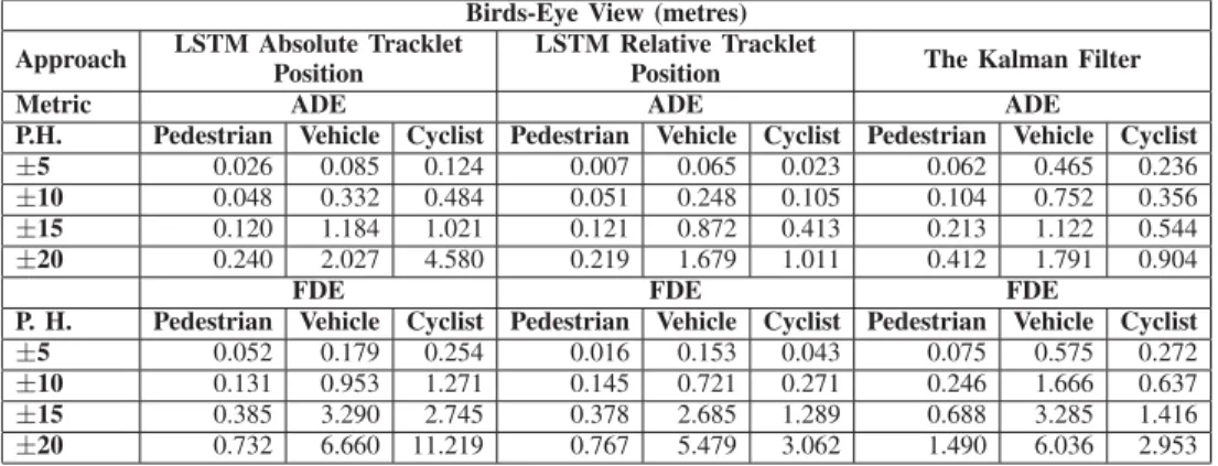
TABLE II

PATH PREDICTION ACCURACY USING BIRDS-EYE VIEW(REAL WORLD MEASURES)

Birds-Eye View (metres) Approach LSTM Absolute Tracklet

Position

LSTM Relative Tracklet

Position The Kalman Filter

Metric ADE ADE ADE

±5 0.026 0.085 0.124 0.007 0.065 0.023 0.062 0.465 0.236 ±10 0.048 0.332 0.484 0.051 0.248 0.105 0.104 0.752 0.356 ±15 0.120 1.184 1.021 0.121 0.872 0.413 0.213 1.122 0.544 ±20 0.240 2.027 4.580 0.219 1.679 1.011 0.412 1.791 0.904

FDE FDE FDE

P. H. Pedestrian Vehicle Cyclist Pedestrian Vehicle Cyclist Pedestrian Vehicle Cyclist

±5 0.052 0.179 0.254 0.016 0.153 0.043 0.075 0.575 0.272 ±10 0.131 0.953 1.271 0.145 0.721 0.271 0.246 1.666 0.637 ±15 0.385 3.290 2.745 0.378 2.685 1.289 0.688 3.285 1.416 ±20 0.732 6.660 11.219 0.767 5.479 3.062 1.490 6.036 2.953

TABLE III

IMPROVEMENTS USING IMAGE COORDINATES Image Coordinate (Pixels) Improvement %

LSTM ATP vs LSTM RTP

The Kalman Filter vs LSTM RTP

Metric ADE ADE

P.H. Pedestrian Vehicle Cyclist Pedestrian Vehicle Cyclist

±5 -24.22 -17.24 -31.32 -31.77 -56.25 -34.43 ±10 -34.92 19.05 -95.06 -5.94 -39.58 -44.27 ±15 -14.23 -9.05 -69.51 46.14 -34.49 44.11 ±20 34.51 -5.46 -80.46 81.00 -31.41 252.76

Metric FDE FDE

±5 -22.37 -12.63 -31.69 -21.06 -49.60 -29.64 ±10 -26.37 22.73 -92.52 -6.46 -39.26 -47.37 ±15 -13.13 -3.79 -48.24 30.19 -34.73 30.65 ±20 48.15 -1.81 -83.67 75.26 -30.44 201.47

Position (ATP). Experiments were done for both type of tracklets.

A total of 853 objects were extracted from all the sequences – 167 pedestrians, 649 vehicles and 37 cyclists – for the four

prediction horizons of 5, 10, 15 and 20 frames. The number of tracklets are shown in Table IV for each object on the four prediction horizons (P.H.).

TABLE IV

SIZE OF THE TRAINING DATA FOR ALL FOUR PREDICTION HORIZONS.

Number of Tracklets

P.H. Pedestrian Vehicle Cyclist All ±5 6,933 18,662 1,282 28,138 ±10 5,933 14,591 1,028 22,907 ±15 5,076 11,365 831 18,714 ±20 4,371 9,172 665 15,658

E. Model

The Keras API1 was used to obtain the implementation of the LSTM architecture . To select the parameters a grid search was executed over the whole dataset, including all objects, and the following conﬁguration achieved the best result. One layer was selected since adding more layers does not improve performance, as shown in [17], where they also mention that

(5)

due to their recurrent nature, even a single layer of LSTM nodes can be considered as a deep neural network:

• Number of layers:1.

• Number of neurons: 128.

• Loss: MSE

• Optimizer: Adam.

V. RESULTS

This set of experiments evaluates the performance of a Kalman ﬁlter with Constant Velocity model with an LSTM network on the KITTI dataset. For LSTM’s results, two sets of experiments were executed. One where the tracklets keep their absolute position (ATP) and other where the tracklets are translated to a relative position (RTP). For the Kalman ﬁlter the same two set of experiments was made but the comparison is not shown since the results using ATP vs RTP showed no difference. The performance was calculated on four different prediction horizons (P.H.) and for three different objects – pedestrians, cyclists and vehicles (labelled as Cars, Vans and Trucks). The data for training and testing consists of the center of the object. The results are also provided in image coordinate (pixels) and in birds-eye view (metres). Due to the size of the image (1224 x 370 pixels), the results show large values in the case of image coordinates. Fig. 3 illustrates the approximate real world implication of variations in pixels as applied to the KITTI dataset. Finally, the relative improvement (error reduction) values shown in Table III and V were cal-culated by[(newV alue−originalV alue)/originalV alue]∗

100 where newV alue is the LSTM RTP methodology and

originalV alue is the approach to be compared with. The negative values means that there was an error reduction using the LSTM RTP approach.

A. LSTM ATP vs LSTM RTP

Table I, in the columns two and three, shows the results on image coordinates obtained when executing the LSTM using the two different type of tracklets (ATP and RTP) and Table III depicts the relative improvements.

Table II, in the columns two and three, shows the results on the birds-eye view obtained when executing the LSTM using the two different type of tracklets (ATP and RTP), whilst Table V presents the improvement.

This set of results show clearly that there was error reduc-tion in most of cases when translating the tracklets to relative position (RTP). In a few cases, mostly pedestrians, a slight increase in error was found.

B. The Kalman Filter vs LSTM RTP

Table I, in columns three and four, shows the results on image coordinates obtained by the Kalman Filter and LSTM RTP and Table III depicts the improvement comparing both approaches.

Table II, in the columns three and four, shows the results on birds-eye view obtained when executing the Kalman Filter and LSTM RTP, whilst table V presents the improvement of LSTM

RTP over the Kalman Filter. As in table III, the negative values indicate that there was error reduction using LSTM RTP.

The results show that LSTM RTP outperforms the simple Kalman Filter on most cases, speciﬁcally for vehicle and pedestrians. Also, it can bee seen that LSTM RTP performs better when predicting in birds-eye view compared to using image coordinates.

TABLE V

IMPROVEMENTS INBIRD-EYEVIEW.

Bird-Eye View (Meters) Improvement % LSTM ATP

vs LSTM RTP

The Kalman Filter vs LSTM RTP

Metric ADE ADE

±5 -74.04 -24.05 -81.80 -89.19 -86.05 -90.40 ±10 8.04 -25.19 -78.35 -50.76 -66.97 -70.52 ±15 0.52 -26.35 -59.61 -43.07 -22.26 -24.10 ±20 -8.74 -17.16 -77.92 -46.77 -6.26 11.78

Metric FDE FDE

±5 -68.13 -14.30 -83.02 -78.14 -73.39 -84.16 ±10 10.25 -24.35 -78.64 -41.30 -56.73 -57.41 ±15 -1.86 -18.38 -53.05 -45.06 -18.24 -8.97 ±20 4.82 -17.73 -72.71 -48.52 -9.22 3.71

C. Discussion

The results obtained in this work show that LSTM ap-proaches perform well for predicting the near future paths of objects in the context of cameras mounted on a moving vehicles. It shows also that the performance of this approach is affected by the prediction time horizon, the largest the prediction horizon resulting in the largest errors.

For the LSTM architecture, it clearly can be seen that translating the tracklets to a relative position (RTP) helps the model to learn better to predict. The reason on this could be that, RTP makes the tracklets to be similar in that space and produces more examples for learning. Another important point to note is that predicting in birds-eye view is better than predicting using image coordinate, however 3D information is not always available.

The results also indicate, that this approach is affected by the size of the training data. For instance, for the class Vehicle, LSTMs outperforms the Kalman Filter for all prediction horizons. One probable reason is that for this object class there is a bigger dataset to train, while for the other objects the size of the training data is poor.

Finally, the processing inference time per tracklet for the LSTMs approach was 0.02 tr/ms, 0.032 tr/ms, 0.045 tr/ms, 0.057 tr/ms for prediction time horizon (PH) of ±5 to ±20 respectively. The Kalman Filter processing time was 3.627 tr/ms, 6.961 tr/ms, 11.012 tr/ms, 13.553 tr/ms for PH of±5 to

±20 respectively. All this using a computer with the following features: GPU GeForce GTX 980, CPU Intel® CoreTM i5-4690K CPU @ 3.50GHz x 4, RAM 24GB.

(6)

Fig. 3. Heat maps of 10-100 pixels (left to right) illustrating pixel differences in the real world.

VI. CONCLUSION

This work presented a single-shot prediction approach that uses one LSTM to predict the future position of objects commonly present in trafﬁc scenes. The selected data set was KITTI because of its realistic scenes, such as highways, inter city, vehicles standing, vehicle moving, its different objects and the labelled data in image coordinate and 3D information. The objective of this work was to compare the performance of the commonly used Kalman Filter with the newer options offered by LSTM architectures and analyze some of the potential inﬂuences on their trajectory prediction accuracy by looking at three object classes, four prediction horizons and two different perspectives (image coordinate and birds-eye view).

The results have shown that using an LSTM achieves good performance of up to an ADE of 0.01m for pedestrians, 0.06m for vehicles and 0.02m for cyclists and up to a FDE of 0.016m, 0.15m, 0.04m for the same objects improving the performance of the baseline Kalman Filter. The results also show that the performance is affected by the prediction horizon where the longer the prediction horizon, the bigger the displacement error. The prediction horizon where the approach is most reliable is for ±5 and ±10 for image coordinate and for ±5 to±15 for birds-eye view perspective.

The performance is also affected by the distance of the object to the vehicle and it appears that the prediction is harder when the object is closer to the vehicle. The desired precision and responsiveness will be dictated by the ﬁnal use of the prediction, for instance in risk analysis or collision avoidance systems.

Observing that the size of the data affects significantly the performance of the LSTM and noting the lack of data for path prediction, useful future work would be to apply data augmentation methods to the KITTI dataset and to utilise transfer learning to fine tune a model trained on a larger path and motion dataset for the specific application of moving cameras on vehicles. This work uses positional and observed paths only and the next step will be to combine external data to constrain the path predictions based on real world knowledge.

ACKNOWLEDGMENT

This work has received funding from EU H2020 Project VI-DAS under grant number 690772 and Insight Centre for Data Analytics funded by SFI, grant number SFI/12/RC/2289.

REFERENCES

[1] L. Fletcher, L. Petersson, A. Zelinskyet al., “Driver assistance systems based on vision in and out of vehicles,” inIntelligent Vehicles Sympo-sium, 2003, pp. 9–11.

[2] K. Bengler, K. Dietmayer, B. Farber, M. Maurer, C. Stiller, and H. Winner, “Three decades of driver assistance systems: Review and future perspectives,”IEEE Intelligent Transportation Systems Magazine, vol. 6, no. 4, pp. 6–22, 2014.

[3] P. Dollar, C. Wojek, B. Schiele, and P. Perona, “Pedestrian detection: An evaluation of the state of the art,”IEEE transactions on pattern analysis and machine intelligence, vol. 34, no. 4, pp. 743–761, 2012.

[4] S. Sivaraman and M. M. Trivedi, “Looking at vehicles on the road: A survey of vision-based vehicle detection, tracking, and behavior analysis,” IEEE Transactions on Intelligent Transportation Systems, vol. 14, no. 4, pp. 1773–1795, 2013.

[5] A. Geiger, P. Lenz, C. Stiller, and R. Urtasun, “Vision meets robotics: The KITTI dataset,” The International Journal of Robotics Research, vol. 32, no. 11, pp. 1231–1237, 2013.

[6] N. Schneider and D. M. Gavrila, “Pedestrian path prediction with recursive bayesian ﬁlters: A comparative study,” inGerman Conference on Pattern Recognition. Springer, 2013, pp. 174–183.

[7] K. Okamoto, K. Berntorp, and S. Di Cairano, “Similarity-based vehicle-motion prediction,” in 2017 American Control Conference (ACC). IEEE, 2017, pp. 303–308.

[8] R. Madhavan, Z. Kootbally, and C. Schlenoff, “Prediction in dynamic environments for autonomous on-road driving,” inControl, Automation, Robotics and Vision, 2006. ICARCV’06. 9th International Conference on. IEEE, 2006, pp. 1–6.

[9] R. E. Kalman, “A new approach to linear ﬁltering and prediction problems,” Journal of basic Engineering, vol. 82, no. 1, pp. 35–45, 1960.

[10] X.-B. Jin, T.-L. Su, J.-L. Kong, Y.-T. Bai, B.-B. Miao, and C. Dou, “State-of-the-Art mobile intelligence: Enabling robots to move like humans by estimating mobility with artiﬁcial intelligence,” Applied Sciences, vol. 8, no. 3, p. 379, 2018.

[11] C. G. Keller and D. M. Gavrila, “Will the pedestrian cross? a study on pedestrian path prediction,”IEEE Transactions on Intelligent Trans-portation Systems, vol. 15, no. 2, pp. 494–506, 2014.

[12] D. Vasquez and T. Fraichard, “Motion prediction for moving objects: a statistical approach,” inProceedings of the IEEE International Confer-ence on Robotics and Automation (ICRA), vol. 4, 2004, pp. 3931–3936. [13] B. T. Morris and M. M. Trivedi, “Learning and classiﬁcation of trajecto-ries in dynamic scenes: A general framework for live video analysis,” in Advanced Video and Signal Based Surveillance, 2008. AVSS’08. IEEE Fifth International Conference on. IEEE, 2008, pp. 154–161. [14] Y. Yoo, K. Yun, S. Yun, J. Hong, H. Jeong, and J. Young Choi, “Visual

path prediction in complex scenes with crowded moving objects,” in Proceedings of the IEEE Conference on Computer Vision and Pattern Recognition, 2016, pp. 2668–2677.

[15] J. Bian, D. Tian, Y. Tang, and D. Tao, “A survey on trajectory clustering analysis,”arXiv preprint arXiv:1802.06971, 2018.

[16] A. Alahi, K. Goel, V. Ramanathan, A. Robicquet, L. Fei-Fei, and S. Savarese, “Social LSTM: Human trajectory prediction in crowded spaces,” inProceedings of the IEEE conference on computer vision and pattern recognition, 2016, pp. 961–971.

[17] F. Altch´e and A. de La Fortelle, “An LSTM network for highway trajectory prediction,” in2017 IEEE 20th International Conference on Intelligent Transportation Systems (ITSC). IEEE, 2017, pp. 353–359. [18] F. Bartoli, G. Lisanti, L. Ballan, and A. Del Bimbo, “Context-aware

trajectory prediction,” in2018 24th International Conference on Pattern Recognition (ICPR). IEEE, 2018, pp. 1941–1946.

[19] B. Kim, C. M. Kang, J. Kim, S. H. Lee, C. C. Chung, and J. W. Choi, “Probabilistic vehicle trajectory prediction over occupancy grid map via recurrent neural network,” in2017 IEEE 20th International Conference on Intelligent Transportation Systems (ITSC). IEEE, 2017, pp. 399–404. [20] A. Bhattacharyya, M. Fritz, and B. Schiele, “Long-term on-board prediction of pedestrians in trafﬁc scenes,” in1st Conference on Robot Learning, 2017.