Meteorological forcing data for urban
outdoor thermal comfort models from a
coupled convective boundary layer and
surface energy balance scheme
Article
Published Version
Creative Commons: AttributionNoncommercialNo Derivative Works 3.0
Open Access
Onomura, S., Grimmond, C. S. B., Lindberg, F., Holmer, B.
and Thorsson, S. (2015) Meteorological forcing data for urban
outdoor thermal comfort models from a coupled convective
boundary layer and surface energy balance scheme. Urban
Climate, 11. pp. 123. ISSN 22120955 doi:
https://doi.org/10.1016/j.uclim.2014.11.001 Available at
http://centaur.reading.ac.uk/38730/
It is advisable to refer to the publisher’s version if you intend to cite from the
work.
Published version at: http://dx.doi.org/10.1016/j.uclim.2014.11.001To link to this article DOI: http://dx.doi.org/10.1016/j.uclim.2014.11.001
Publisher: Elsevier
All outputs in CentAUR are protected by Intellectual Property Rights law,
including copyright law. Copyright and IPR is retained by the creators or other
copyright holders. Terms and conditions for use of this material are defined in
the End User Agreement
.
www.reading.ac.uk/centaur
CentAUR
Central Archive at the University of Reading
Reading’s research outputs online
Meteorological forcing data for urban outdoor
thermal comfort models from a coupled
convective boundary layer and surface energy
balance scheme
S. Onomura
a,⇑, C.S.B. Grimmond
b, F. Lindberg
a, B. Holmer
a, S. Thorsson
aaDepartment of Earth Sciences, University of Gothenburg, Gothenburg, Sweden bDepartment of Meteorology, University of Reading, Reading, United Kingdom
a r t i c l e
i n f o
Article history: Received 19 February 2014 Revised 22 July 2014 Accepted 4 November 2014 Keywords: Boundary layer Urban land surface model Surface energy balance Outdoor thermal comforta b s t r a c t
Site-specific meteorological forcing appropriate for applications such as urban outdoor thermal comfort simulations can be obtained using a newly coupled scheme that combines a simple slab convec-tive boundary layer (CBL) model and urban land surface model (ULSM) (here two ULSMs are considered). The former simulates daytime CBL height, air temperature and humidity, and the latter estimates urban surface energy and water balance fluxes accounting for changes in land surface cover. The coupled models are tested at a suburban site and two rural sites, one irrigated and one unirrigated grass, in Sacramento, U.S.A. All the variables modelled compare well to measurements (e.g. coefficient of determination = 0.97 and root mean square error = 1.5°C for air temperature). The current version is applicable to daytime conditions and needs initial state condi-tions for the CBL model in the appropriate range to obtain the required performance. The coupled model allows routine observa-tions from distant sites (e.g. rural, airport) to be used to predict air temperature and relative humidity in an urban area of interest. This simple model, which can be rapidly applied, could provide urban data for applications such as air quality forecasting and building energy modelling, in addition to outdoor thermal comfort.
Ó2014 The Authors. Published by Elsevier B.V. This is an open access article under the CC BY-NC-ND license ( http://creativecom-mons.org/licenses/by-nc-nd/3.0/).
http://dx.doi.org/10.1016/j.uclim.2014.11.001
2212-0955/Ó2014 The Authors. Published by Elsevier B.V.
This is an open access article under the CC BY-NC-ND license (http://creativecommons.org/licenses/by-nc-nd/3.0/).
⇑Corresponding author at: Gothenburg Urban Climate Group, Department of Earth Sciences, University of Gothenburg, Box 460, Gothenburg SE-405 20, Sweden.
E-mail address:shiho.onomura@gu.se(S. Onomura).
Contents lists available atScienceDirect
Urban Climate
1. Introduction
Heat waves, such as the ones which occurred in Eastern Europe in 2010, North America and Australia in 2012, and China in 2013, are expected to have a large impact on human health, well-being and economic burden in the future (IPCC, 2012). Urban areas are particularly vulnerable to such effects given the density of urban populations and the compounding effect of the urban heat island, which will grow with increased population and greater urbanisation (McMichael et al., 2006; Pascal et al., 2006). To inform climate sensitive planning, intra-urban climate conditions at local (102–104m, e.g. a district) and micro-scales (101–103m, e.g. a street canyon) need to be predicted for building energy applications and for estimating outdoor human thermal comfort in cities.
The thermal comfort at the neighbourhood to street level scale is chiefly influenced by urban struc-tures. It varies greatly within short distances due to shadow patterns generated by urban surface geometry and radiative properties related to materials and urban density (Lindberg and Grimmond, 2011a). For the estimation of thermal comfort, micro-scale modelling of mean radiant temperature (Tmrt) is essential (Lindberg et al., 2008; Matzarakis et al., 2010). TheTmrt, which describes the radiant
(short-wave and long-wave) heat exchange between a person and his or her surroundings, is defined as the ‘uniform temperature of an imaginary enclosure in which the radiant heat transfer from the human body equals the radiant heat transfer in the actual non-uniform enclosure’ (ASHRAE, 2001). It is considered to be one of the most important meteorological variables governing the human energy balance and thermal comfort outdoors, especially during clear and calm summer days (Mayer and Höppe, 1987).
Generally, in order to modelTmrt for the area of interest, the required meteorological variables
(short-wave radiation, air temperature, and humidity) are obtained from observations or models. However, they are often not specific for the site (e.g. they are often derived from an airport), or rely on the use of long-term mean variables rather than typical sequences of conditions. When data from other areas are used (Erell and Williamson, 2006; Lindberg et al., 2013), often it is assumed that both areas are exposed to the same regional conditions and land surface effects on the meteorological vari-ables are ignored. As a result, these local-scale land cover and land use characteristics systematically impact the accuracy ofTmrtcalculations. If data are derived from atmospheric numerical simulation,
sometimes with coupled urban land surface schemes (Miao et al., 2009; Flagg and Taylor, 2011; Loridan et al., 2013), this requires large computational cost.
Currently, only a few urban land surface models (ULSMs) are set up to rapidly calculate site-specific air temperature within or above the canopy layer (Swaid and Hoffman, 1990; Erell and Williamson, 2006; Bueno et al., 2012; Bueno et al., 2013; Stewart et al., 2013). Of these, onlyBueno et al. (2013) andStewart et al. (2013) take feedback from the land surface to the meso-scale atmosphere into account. Both use the Town Energy Balance (TEB) scheme (Masson, 2000) coupled to different bound-ary layer models.
In order to investigate daytime human thermal comfort in cities, simple methods to obtain more site-specific input meteorological variables need to be explored. In this study a scheme is developed to provide daytime meteorological variables representative of an urban area for a micro-scale urban radiation model to simulateTmrt. A meso-scale slab convective boundary layer (CBL) model is coupled
to two local-scale ULSMs (Section2). Of interest is the ability of the combined model to simulate meteorological variables, accounting for land surface changes, using minimal computer resources (e.g. a personal computer), and simple inputs around meteorology, land surface cover, and initial state conditions. The number of meteorological inputs is reduced compared to those required for the sep-arate models included in the coupled scheme. The coupled models are tested at three sites (suburban, irrigated sod-farm and unirrigated grassland) in Sacramento, CA (Sections3 and 4). They replicate well the local-scale urban meteorological variables (air temperature and relative humidity) from those measured at rural sites (Section6). Here the focus application is to obtainTmrt, one of most critical
components of outdoor human comfort, by calculation with a micro-scale urban radiation model – the SOlar and Long Wave Environmental Irradiance Geometry model (SOLWEIG) (Lindberg et al., 2008; Lindberg and Grimmond, 2011b). SOLWEIG determines three-dimensional radiation fluxes
andTmrt. To ensure that the coupled model can provide robust input for this application, sensitivity
tests are undertaken with SOLWEIG (Section5.1 and 6). The coupled model scheme developed is applicable to urban climate sensitive planning issues such as the effect of land cover changes on intra urban temperature variations; building energy applications; air quality forecasting; and dispersion modelling.
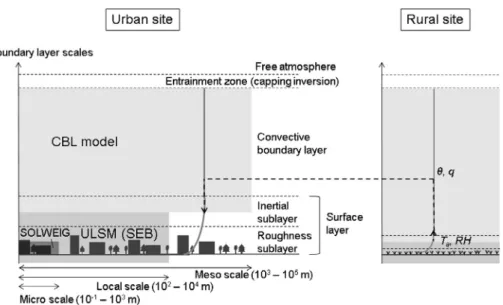
2. The convective boundary layer and urban land surface models
The convective boundary layer (CBL) is strongly influenced by daytime momentum, heat, moisture and air pollutant exchanges in the urban environment. The depth of this mixing layer determines the volume for dilution of heat, water, carbon, and other atmospheric pollutants and their dispersion downwind of the city. The CBL is capped at its top by a temperature inversion and an entrainment zone (Fig. 1). Here, a simple approach to derive the growth of the CBL, the so-called ‘‘slab’’ model based on thermodynamic processes is used. The rate of change of air temperature and humidity within the CBL are determined from the turbulent heat fluxes and the net fluxes from the entrainment zone (Raupach, 2000). Formulated at the meso-scale (103–105m), the slab model determines the height of the CBL (zi), potential temperature (h), and specific humidity (q) through time (t), using the
conser-vation equations of heat and water vapour (e.g.Cleugh and Grimmond, 2001):
@h @t¼ QH
q
Cpziþ hþh zi dzi dt ws ð1Þ @q @t¼ QEq
LvZi þqþq zi dzi dt ws ð2Þ whereQHandQEare turbulent sensible and latent heat fluxes at the surface,q
Cpis the heat capacity ofair,Lvis the latent heat of vaporization,h+andq+are the potential temperature and specific humidity
just abovezi, andwsis the subsidence velocity of air. The rate of change ofhandqwithin the CBL is
derived from temporally integrating the conservation equations. The CBL changes its height, zi, in
response to changes in surface heat fluxes and entrainment across the capping inversion at the top of the CBL. A number of different encroachment and entrainment schemes exist (e.g. Tennekes,
Fig. 1.Relation between boundary layer scales, the models and observations in this study: the convective boundary layer (CBL), surface energy balance (SEB) and micro-scale radiation environment (SOLWEIG), urban land surface model (ULSM).
1973; Tennekes and Driedonks, 1981; McNaughton and Spriggs, 1986; Rayner and Watson, 1991), includingTennekes and Driedonks (1981):
dzi
dt ¼
b1w3þb2u3 zi
D
hvghv1ð3Þ whereb1andb2are constants,w⁄andu⁄convective and friction velocities,hvandDhvvirtual potential
temperature and the temperature difference across the capping inversion.
In this study, to determine the surface fluxesQHandQE, two ULSMs are used: the Surface Urban
Energy and Water balance Scheme (SUEWS) (Järvi et al., 2011) and the Large-scale Urban Meteorolog-ical Parameterization Scheme (LUMPS) (Grimmond and Oke, 2002; Loridan et al., 2010). Both calculate the urban surface energy balance (Oke, 1988):
QþQF¼QHþQEþ
D
QS ½W m 2ð4Þ
whereQ⁄is the net all-wave radiation,Q
Fthe anthropogenic heat flux, andDQSthe net storage heat
flux. SUEWS uses a surface resistance based Penman Monteith approach, whereas LUMPS uses the de Bruin and Holtslag (1982)simplification of Penman Monteith to calculateQHandQE. The ULSMs
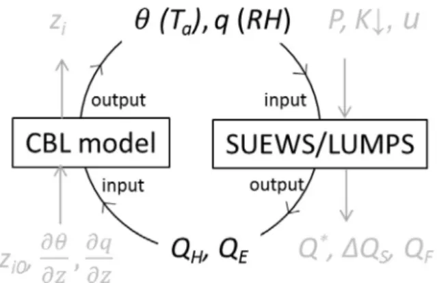
are local-scale models (Fig. 1) applicable to a horizontal spatial extent of the order 102–104m. The ver-tical extent is from the depth where there is no net exchange of heat over the period of interest to the top of the roughness sub-layer (which is approximately the lowest atmospheric layer for meso-scale boundary layer models). Both ULSMs require land cover information and meteorological data (air tem-perature, air humidity, incoming short-wave radiation, wind speed, and air pressure) at the local-scale. In this study, the models have been coupled so that the CBL model calculateshandqusingQHand
QEfrom the ULSMs, while SUEWS and LUMPS estimate the surface heat fluxes using air temperature
(Ta) and relative humidity (RH) obtained from the CBL modelledhandqin the previous time step
(Fig. 2). The combined model is forced by incoming short-wave radiation (K;), atmospheric pressure (P) and wind speed (u), and the need forh(andTa),q(andRH),QHandQEare eliminated. However, as
the CBL model is for convective growth, it is limited to daytime conditions only. The entrainment schemes require initial values ofh,q, andzi(i.e.h0,q0, andzi0) and the vertical gradients ofhandq
(@h/@zand@q/@z) allow the estimation of the net fluxes from the entrainment zone for each time step (second term on right-hand-side of Eqs.(1) and (2)). The initial data,@h/@zand@q/@zrequire vertical information which may be obtained from radiosonde measurements (Section3.1), re-analysis data (e.g.ERA-interim) or model output (e.g. numerical weather prediction,NWP). Radiosonde data are generally sparse, especially so in urban areas.h0andq0can be assessed from fixed measurements
at the height of inertial sublayer. However,zi0,@h/@z, and@q/@zare difficult to assess as measurements
at the top ofziare needed. Therefore the parameterizations or default values ofzi0,@h/@zand@q/@z
Fig. 2.Core structure with forcing input data (grey) and output (grey) from the coupled CBL model and SUEWS/LUMPS models linked viah,q,QHandQE. For definition of notation seeAppendix.
may be required to apply the coupled models in practice. To address this, we present a sensitivity test ofzi0,@h/@zand@q/@z(Section5.2).
The CBL model and ULSMs potentially have different horizontal scales (Fig. 1). Here, the surface parameters for the ULSMs are assumed to be representative of the same horizontal scale as the scale of the CBL model. An alternative approach would be for the CBL model to use regionally averaged heat fluxes calculated by the ULSMs for several local-scale areas.
3. Procedures for model evaluation
3.1. Observation data
To evaluate the performance of the coupled models, meteorological data measured at a suburban site (SU) as well as dry and wet rural sites (referred to as DR and WR, respectively) in Sacramento (Fig. 3) California, U.S.A. between 20th and 29th August 1991 are used (Grimmond et al., 1993). The observation period was characterised by clear skies and warm weather. The DR area was unused and covered with tall, extremely dry grass, whereas WR was an extensive sod farm with short, irri-gated grass.
At the three sites basic meteorological variables (Ta,RH,u,P, etc.), net all-wave radiation and heat
fluxes were measured. The heat fluxes were determined by eddy covariance techniques. The measure-ment heights for each variable at each site are given inTable 1. Details of the measurement techniques and data processing are provided inGrimmond et al. (1993)andGrimmond and Oke (1995). During 22nd–24th and 26th–28th August, free flying radiosondes were released at SU (see Table I in Cleugh and Grimmond, 2001) from which initial values of@h/@z,@q/@z, andziwere derived. Herezi
is defined by a potential temperature inversion. AsK;was not directly measured at SU, it is obtained from data produced for Sacramento Metropolitan Airport (AP), 9.3 km away, using the METSTAT solar radiation model (NREL, 2012). These data are used for all periods except for the morning of 24th August, when the METSATK;appeared to be unusually small compared to the observedQ⁄, suggesting
Fig. 3.Location of suburban (SU), dry rural (DR), wet rural (WR) and airport sites on a satellite image of Sacramento on 10th August 2006 (Landsat, 2006). Red line delimits the urban area. (For interpretation of the references to colour in this figure legend, the reader is referred to the web version of this article.)
Table 1
Model options and parameter values used. For definitions of notation seeAppendix A. CBL model options
Subsidence velocity 0.01 m s1 Entrainment scheme Tennekes and
Driedonks (1981) ———————————————————————————————————————————————————————————————————
Time zone (h)8 (to UTC)
Day light saving time & external water use (DoY)
97–300 Site-related variables Urban site Dry site Wet site
Period (DoY) 232–241 234–241 234–241
Latitude, Longitude 38°390N, 121°190W 38°330N, 121100W 38°310N, 121410W
Asurface(ha) 78 (a 500 m radius circle area)
10 10
Population density (in ha-1
) 18 0 0
Land cover (plan area fractionf): (Grimmond and Oke 1999a)
fauto irrigation 0.0098 0 0 fbuilding 0.351 0 0 fconiferous vegetation 0.064 0 0 fdeciduous vegetation 0.064 0 0 firrigated grass 0.349 0 1 fpavement/impervious 0.115 0 0 fsoil 0.005 0 0 funirrigated grass 0 1 0 fwater 0.052 0 0
Roughness length for momentum:
z0m(m)
Macdonald et al. (1998)
0.05 0.005
Zero plane displacement:zd(m) Macdonald et al. (1998)
0.15 0.035
Roughness length for heat and Water vapour:zov(m)
Kawai et al. (2009) Kawai et al. (2009) Kawai et al. (2009)
Mean building height:zh(m) 5.201 0 0
Mean vegetation height:zhv(m) 8.369 0.5 0.05
Height of the wind speed measurement:zm(m)a
9 1.8 1.3
Frontal area index:(Grimmond and Oke 1999b)
Building 0.058 0 0
Tree 0.185 0 0
———————————————————————————————————————————————————————————————————
Submodel option Urban site Dry site Wet site
Q⁄ L;is calculated by usingT
aandRHLoridan et al. (2011) Effective surface albedo of sub-surfaces (Oke, 1987)
abuilding 0.27 aconifer 0.1 adeciduous 0.18 agrass 0.3 apavement 0.2 awater 0.7
QH,QELUMPS parametersb a= 0.55 b= 3 a= 0.19 b= 3 a= 1.0 b= 20
QESUEWS conductance air temperature limits (Järvi et al., 2011, Eq. (17))
TH(°C) 50 TL(°C) 0
DQsObjective hysteresis model (OHM)Grimmond et al. (1991)using the modelledQ⁄
OHM coefficients a1 a2 a3 0.83 0.83 24.6 Pavedc a 1= 0.21d a2= 0.11 a3=16.9 a1= 0.35d a2= 0.03 a3=26.0 0.1 0.23 6 Buildingc 0.34 0.31 31.4 Treec 0.32 0.54 27.4 Grassc 0.33 0.07 34.9 Soilc 0.50 0.21 39.1 Waterc
QFprofiles AHDIUPRF1 and 2
(Järvi et al., 2014)
– –
Stability function
Momentum: Unstable Högström (1988)modified fromDyer (1974)
Stable Van Ulden and Holtslag (1985)
the flux may be responding to different local sky conditions. Thus for this period only, theK;data are replaced by: K#repðtÞ ¼QðtÞ K# Q ð5Þ using the mean diurnal relation between observedK;andQ⁄for the measurement period.
The soil heat flux was measured at the three sites using Campbell Scientific heat flux plates installed at 0.07 m depth with CSI TCAV temperature sensors above to account for heat divergence. Corrections are made for soil moisture content using both gravimetric and time domain reflectometry measurements.
3.2. Model settings
The complete model of the CBL provides results using SUEWS and LUMPS. For clarity we refer to these as BLUEWS (CBL model + SUEWS) and BLUMPS (CBL model + LUMPS). The model is executed according to the procedures in the manual (Järvi et al., 2014), using the options summarised inTable 1. The land cover fraction values (f) are constant for the study period.
Q⁄is forced byK;(Offerle et al., 2003; Loridan et al., 2010), with incoming long-wave radiation (L;) determined fromTaandRH. LUMPS
a
andbparameters forQHandQEshown inTable 1are calculatedbased on the surface type. LUMPS is confirmed to have the same performance for SU asGrimmond and Oke (2002)(their Table 7). However, we found thatb= 20 W m2often used for verdant vegetation is too high for DR, given the extremely dry conditions at that site. This parameter is based on observa-tions over agricultural land (Hanna and Chang, 1992). Lowerbimproves the performance of LUMPS for surface heat fluxes at DR, therefore hereb= 3 is used for less vegetated sites in LUMPS.DQSis
calcu-lated as a function of the modelledQ⁄and surface materials based on the Objective Hysteresis Model (OHM) (Grimmond et al., 1991; Grimmond and Oke, 1999c). At SU, the OHM coefficients used are based on characteristics of the plan area surface cover (Table 1). For the rural sites, it is possible to determine the coefficients (Grimmond and Oke, 1999c) as the observed soil heat flux and net all-wave radiation data are available (Tables 1 and 2, and Section4).QFfor SU is estimated using the method of
Järvi et al. (2011), with the same diurnal profile as determined from Vancouver data (Grimmond, 1992) (see Table 1 ofJärvi et al., 2011).
The SUEWS surface resistance coefficients used are theJärvi et al. (2011)median values (50th per-centile) based on a number of urban and suburban locations. The stability functions for momentum, heat and moisture used are those ofHögström (1988), modified fromDyer (1974)andVan Ulden and Holtslag (1985). Roughness length for momentum (z0m) and zero plane displacement length (zd) are
calculated within SUEWS for SU based on morphometric characteristics (Macdonald et al., 1998; Initial soil stores 100 mm
(120 mm only for irrigated grass)
1.5 mm for unirrigated grass (0 mm for the others)
111 mm for irrigated grass (0 mm for the others)
Initial surface stores 0 mm 0 mm 0 mm
Maximum soil moisture 150 mm 150 mm 150 mm
External water use (Ie) Modelled byJärvi et al. (2011) None Observation
Ieprofile 00:00 to 06:00 h 0.036
07:00 to 03:00 h 0.044 04:00 to 19:00 h 0.050 20:00 to 23:00 h 0.036
a
Air temperature, relative humidity, and air pressure were also measured at this height. The turbulent heat fluxes and all-wave radiation were measured at 29 m at SU and at the specified heights at the other two sites. Soil heat flux plates were installed at0.068 and0.07 m from ground surface at DR and WR sites, respectively.
b Note these are the effective parameters that are calculated in LUMPS.
c References areAnandakumar (1999)for pavement,Meyn and Oke (2009)roof, average of all seven sources inGrimmond
and Oke (1999c)tree,Doll et al. (1985)grass,Fuchs and Hadas (1972)soil,Souch et al. (1998)water.
d
Grimmond and Oke, 1999b) and based on estimates using observed mean grass height (Grimmond et al., 1993) for the rural sites (Table 1). Roughness lengths for heat and water vapour are calculated based onKawai et al. (2009).
Irrigation is regulated in Sacramento with alternating (odd/even) properties allowed to irrigate on 6 days of the week, with no irrigation permitted on Sundays (25th August) (Grimmond et al., 1993). The external water supply (or irrigation,Ie) is modelled for SU using Eq.(5)ofJärvi et al. (2011)for
the daily total and within dayIe profile (Table 1). The sod-farm (WR)Ieis based on the patterns
observed during the fieldwork. As it has been demonstrated that urban land surface models, like their rural counterparts, need to ensure appropriate soil moisture conditions (Best and Grimmond, 2013), a spin up period of three times the study length was used. This is assumed to be most critical for SU and WR, as the natural grassland (DR) had extremely low (<2%) soil moisture, so an initial value of 1.5 mm was used. This proposed model has the advantage, compared to more complex models, that the addi-tional computer time is insignificant, whereas for others the constraint of inadequate spin up time may need to compromise performance.
The subsidence velocity across the capping inversion of the entrainment zone for the CBL growth is set to0.01 m s1
(Cleugh and Grimmond, 2001). TheTennekes and Driedonks (1981)entrainment scheme, as recommended byCleugh and Grimmond (2001), is used. The initial evaluation (Section 4) uses the@h/@zand@q/@zvalues based on the measured profiles, but during the sensitivity tests (Sec-tion5) the effect of constant values based on the radiosonde measurements is assessed.
The model is run continuously (20th–29th August for SU; 22th–29th August for DR and WR) with the CBL model during the day and the ULSMs forced by observations at night. By usingh0,q0,zi0,@h/@z,
and@q/@z(see Sections2 and 3.1), the CBL model is initialized based on the calculated sun zenith angle (>85°) and modelled sensible heat flux (>0 W m2
). All calculations are conducted using local apparent time. Initial values ofh0andq0for the rural sites use measured air temperature and humidity. Forzi0,
@h/@zand@q/@z, the SU radiosonde measurements are used for all the three sites given they are not available for the rural sites. However, these values are expected to be different at the rural sites; nota-blyzi0is expected to be lower and to differ between the rural sites. To evaluate SUEWS/LUMPS with
the flux observations, a 1 h time step is needed. The ULSMs use a smaller time step (e.g. 5 min) to ensure an appropriate response relative to the water inputs (precipitation, irrigation). However, the CBL takes a longer time to adjust its properties at the meso-scale, overca.10–30 min (Cleugh and Grimmond, 2001). So the CBL calculations ofzi,h, andqare performed at 15 min intervals using
lin-early interpolated data to reduce the error when the conservation equations are temporally integrated.
3.3. Model evaluation
The performance of the model, evaluated using observations from the three sites (SU, DR, and WR), is assessed without CBL feedback (referred to as SUEWS and LUMPS) and with CBL feedback (BLUEWS and BLUMPS). One code with different options selected (Järvi et al., 2014) is used with the input data and parameter settings. The focus is onQHandQE,handqwithin the CBL, andzifor 1 h intervals during
the daytime.
The statistics used for evaluation are the root mean square error (RMSE) and the coefficient of determination (R2). The results for SU are also compared toCleugh and Grimmond (2001)(referred to as CG01) model results with the same entrainment scheme (Tennekes and Driedonks, 1981). Table 2
Objective hysteresis model coefficients (a1, a2and a3) for unirrigated and irrigated grassed areas determined from fitting Eq.(3)in
Grimmond and Oke (1999c)using observed net all-wave radiation to observed soil heat fluxes at the dry rural and wet rural sites in Sacramento.Nis the number of hours of data used.
Description Coefficients Statistical performance
a1[–] a2[s] a3[W m2] N Slope Intercept R2 RMSE[W m2]
Dry, long grass 0.214 0.114 16.85 189 0.838 1.4 0.84 20.7
CG01 obtained the friction velocityu⁄using the logarithmic wind profile with observeduand atmo-spheric stability functions for momentum (same as Table 1) and roughness parameters (z0, zd,
Grimmond and Oke, 1999b). CG01 obtained the atmospheric stability using the method given in Grimmond and Cleugh (1994). CG01 initialized CBL calculations when QH became positive after
05:00 and used a time step interval of 15 min for calculations.
4. Performance of the coupled model
The turbulent heat fluxes modelled using BLUEWS and BLUMPS are almost identical to those of SUEWS and LUMPS for SU and DR, differing only forQHat WR (Fig. 4). Almost all heat fluxes are
under-estimated relative to the observations during periods when these fluxes are large, while they are over-estimated when fluxes are small. This trend in turbulent heat fluxes is also noted byJärvi et al. (2011). BLUEWS has a largerRMSEthan BLUMPS for SU and WR where evaporation occurs. Larger evaporation rates are driven by stronger convective mass transfer under unstable conditions if water is available, e.g. as occurred on 22nd–24th August, compared to 26th–28th (not shown). Thus it is dependent on the surface water balance, e.g. soil moisture and external water use, which is accounted for in SUEWS but not in LUMPS. Unfortunately, there is no independent water use data to evaluate these compo-nents of the SUEWS model. However, specification of soil moisture initial conditions has been found to be important generally in ULSMs (Best and Grimmond, 2013). As the water availability for evapo-ration changes with the land surface characteristics, a sensitivity test is conducted (Section5.2). The relatively largeRMSEof SUEWS /BLUEWSQHresults from the variance ofQEasQHis calculated as the
residual of the surface energy balance.Järvi et al. (2011), who found this same trend in SUEWS, noted the QEvariance is acceptable compared to the original model ofGrimmond and Oke (1991)since
SUEWS reduces the input data so much. For the DR site (Fig. 4e–h), both BLUEWS and BLUMPS model
Fig. 4.Modelled sensible and latent fluxes (QH,QE) (1 h) versus the observations for uncoupled (LUMPS, SUEWS, grey) and
coupled (BLUMPS, BLUEWS, black) runs for (a–d) suburban (e–h) dry rural and (i–l) wet rural. Model statistics (R2
,RMSE, linear regression) are shown.
QHwell, while BLUEWS underestimates and BLUMPS overestimatesQE. The extreme environment of
DR results in excessively high surface resistance values in SUEWS/BLUEWS, and thus almost no evapo-transpiration occurs (observed values less than 70 W m2). However, since the rate ofQ
Eat DR is very
small, it has a very small impact on the modelling ofQHandDQS. For the WR site (Fig. 4i–l), both runs
have good performance forQE, but the coupledQHresults are poorer than the uncoupled results. The
OHM coefficients used for modellingDQSat the rural sites are calculated using regression analysis for
the observedDQS and Q⁄. The performance of the modelledDQS using these coefficients and the
observedQ⁄compared to the observations areR2= 0.84 and 0.88, butRMSE= 20.7 and 39.2 W m2 for DR and WR, respectively (Table 2).
When the modelledzi,handqwithin the CBL at SU are compared to the radiosonde observations and
the CG01 CBL results, all runs show good overall performance (Fig. 5). The performance of the coupled runs is good forziandh(R2andRMSE), but it is poorer forq. The complex observedqprofiles (e.g. for
August 24th, seeFig. 8in CG01) are almost impossible for a simple slab model to predict. Given that BLU-EWS performs better than BLUMPS for q (R2= 0.61, RMSE= 1 g kg1; R2= 0.48, RMSE= 1.2 g kg1, respectively), the results support the use of the biophysical evaporation model SUEWS.
As expected, at DR larger growth ofziandhand decreasingq(Fig. 6) compared to SU are modelled
(Fig. 5), while smaller growth ofziandhand increasingqat WR are predicted. The BLUMPSqis much
larger than that derived from BLUEWS becauseQE is overestimated (underestimated) by BLUMPS
(BLUEWS) (Fig. 4).
5. Sensitivity tests
Three sensitivity tests are conducted here. First, given an intended application of the coupled model is to force the micro-scale urban radiation model SOLWEIG (Lindberg et al., 2008; Lindberg and Grimmond, 2011a), we assess the impact ofTaandRHon SOLWEIG modelledTmrt.Second, as
the land cover characteristics influence all the surface energy balance fluxes, the changes in land cover
Fig. 5.Modelled convective boundary layer height (zi), potential temperature (h) and specific humidity (q) during 22nd–28th in August 1991 using the coupled runs (BLUEWS, BLUMPS) for suburban Sacramento with theCleugh and Grimmond (2001) results and the radiosonde observations also shown. Modelled results plotted hourly.
and height of the roughness elements are explored. Third, as the coupled runs require the not easily obtained (Section2) initial values ofzi0,@h/@zand@q/@z(Eqs.(1) and (2)) as forcing data for the CBL
model, the parameterizations or default values may be required to apply the coupled models in prac-tice. The impact of the alternative options on the modelledTaandRHare explored.
5.1. SOLWEIG
SOLWEIG is run for the period 11:00–14:00 local apparent time with a standing person whose cen-tre of gravity is at a height of 1.1 m (this equates to an ‘average’ person of 1.80 m height and 75 kg weight), located within a simple canyon with a sky view factor of 0.6.
For the base run (S0), observedTa,RH, andK;are compared to changes to the observed values ofTa
± 10°C (S1) andRH± 20% (S2) (Table 3a). Changes in calculated mean radiant temperature (DTmrt)
indicate the model is more sensitive toTathanRH(Fig. 7). Therefore for simplicity, the variations of
RHassociated with the changes ofTaare ignored. The change inDTmrtforTais nearly linear, with a
1°C error inTaproducing a 0.84°C impact onTmrt. This is equal to the effect caused by about a 28%
error inRH. Considering the smallRHimpact onTmrtcompared toTa, the temperature dependency
ofRHis ignored in this analysis. Thus, good estimation ofTais more critical to accurately estimateTmrt
than good estimate ofRH(i.e. q). 5.2. SUEWS land cover characteristics
Section4shows that SUEWS modelledQEis sensitive to land surface characteristics. To examine
the influence of land cover changes, sensitivity tests are performed, which include shifting land cover fractions between buildings and deciduous trees (termed SW1 inTable 3b), as well as shifting between unirrigated grass and impervious surface (SW2). Additionally, the impact of the heights of buildings and trees (SW3 and SW4) are compared. For the reference run (SW0, presented in Section4), 50% Fig. 6.Hourly modelled convective boundary layer height (zi), potential temperature (h) and specific humidity (q) using the coupled runs (BLUEWS, BLUMPS) for dry rural and wet rural sites (DR, WR) in Sacramento. Wet rural is not modelled on 24th August as the forcing data are missing due to irrigation.
of the 60 min modelledQEhave absolute errors (AE50) of less than 8.0 W m2(Fig. 8). When the frac-tion of deciduous trees increases by 15% (from buildings), the AE50increases to 10.7 W m2(Fig. 8a). Enhancing the irrigated grass by 15% (from pavement) results in AE50 increasing to 11.2 W m2 (Fig. 8b). With taller (+5 m) buildings and trees, AE50is 9.7 and 9.0 W m2, respectively (Fig. 8c and d). Taller buildings and trees increasez0andzd, influencing convective transfers. These impacts are
smaller than changes in the grass fraction, as larger grass fraction (from pavement) expands the water availability for evaporation, which impacts the modelledQE.
The land cover changes influence the maximum (absolute) errors (Fig. 8). The AE90(90% of the 60 min modelledQEhave absolute errors) are less than 54.9 W m2on average, whereas AE90is largest
Table 3
Sensitivity tests to evaluate the impact on model performance of (a) SOLWEIG (period 11:00–14:00 h), (b) SUEWS (whole period), and (c) BLUEWS (daytime). Section5provides more details.Appendix Ahas notation defined. Data used: observed (ob), replaced with radiosonde data at convective boundary layer height (ra), and mean of the observations (av).
Run code (a) Variables SOLWEIG T(°C) RH(%) K;(W m2 ) ——————————————————————————————————————————————————————————————————— S0 ob ob ob S1 ±10 of ob, 2°C step ob ob S2 ob ±20 of ob, 2% step ob (b) SUEWS
Land surface characteristics
———————————————————————————————————————————————————————————————————
SW0 Average surface characteristics (Table 1)
SW1 Change land cover: building to deciduous trees (±15%, 5% step)
SW2 Change land cover: irrigated grass to pavement (±15%, 5% step)
SW3 Change height: building (±5 m, 0.5 m step)
SW4 Change height: tree (±5 m, 0.5 m step)
(c) Variables BLUEWS zi0(m) oh/oz(K m1 ) oq/oz(g kg1 m1 ) ——————————————————————————————————————————————————————————————————— B0 ob ob + ra ob + ra B1 ob ob ob B2 av av av B3 100–400, 25 step av av B4 100, 250, 400 0.005–0.09, 0.005 step 0.02 to 0.09, 0.01 step
Fig. 7.Change in calculated mean radiant temperature (Tmrt) for the S0 run to changes in (left) air temperature (Ta) (S1) and (right) relative humidity (RH) (S2) (seeTable 3a and Section5.1).
when grass is increased by 15% (83.1 W m2) and most improved (AE90= 50.5 W m2) when building height is increased by 4 m (Fig. 8). These results are also consistent with analysis of the modelled results by wind direction with hourly source area (Cleugh and Grimmond, 2001) derived land cover characteristics (not shown). This suggests that the source area shape is incorrect in some conditions. 5.3. CBL forcing data
Sensitivity tests are performed to evaluate the impact of using alternatives tozi0,@h/@zand@q/@zon
TaandRHmodelled by BLUEWS (Table 3). The reference analysis (termed B0 inTable 3c, and presented
in Section4) uses the observed values ofzi0,@h/@zand@q/@zgiven at sunrise and considers the change
of@h/@zand@q/@zwith estimatedziat every time step. Thus@h/@zand@q/@zare replaced with the
radiosonde values measured at the height ofziat sunrise. B1 does not consider the change;zi0,@h/
@zand@q/@zare given by the observation at sunrise and are used consistently for all that day. B2 uses the average of initial values observed for the 6 days; these arezi0= 241.5 m,@h/@z= 0.043 K m1and
@q/@z= 0.009 g kg1m1. Thus, the model runs B0 to B2 become more independent of the radiosonde measurements. For these three cases (B0, B1, and B2), BLUEWS, BLUMPS and the uncoupled CBL model are run with all other model settings the same as used in Section4.
In general, B1 and B2 have largerRMSEand smallerR2for all variables than B0 (Fig. 9). The larger error in B1, when radiosonde profile data are unavailable to adjust@h/@zand@q/@zatziat each time
step, indicates these adjustments improve model performance. The B2 results have a smallerRMSE and largerR2for all variables compared to B1. This supports the use of typical values based on bound-ary layer measurements. Overall, BLUEWS and BLUMPS have similar performance to the CG01 CBL model, despite slightly poorer performance for heat fluxes for BLUEWS than BLUMPS. For BLUEWS humidity is better correlated with observations (Section4). Only BLUEWS is assessed in the following
Fig. 8.Impact of changes in surface land cover characteristics on 60 min absolute latent heat flux errors (modelled (m) – observed (o)) cumulative (percent of data) for land cover changes from (a) buildings to deciduous trees, (b) irrigated grass to pavement, (c) building height, and (d) tree height. See key for range of changes used. Dash-line is average used in Section4.
sensitivity tests. BLUEWS has a stronger biophysical base, so it responds to changes in surface water state, which provides the potential for the application of the coupled model system to a wide range of cities and surface water conditions.
The impact ofzi0on the modelledTaandRHis tested withzi0varied from 100 to 400 m in 25 m
increment steps (Table 3c, B3). TheRMSEofTaandRHchange from 1.4 to 2.8°C (minimum when
zi0= 200 m) and 5.5% to 7.0% (minimumzi0= 150 m), respectively (Fig. 10). The impact ofzi0is
rela-tively small onTaand small enough to ignore onRH. Values ofzi0in the range of 100–400 m are
prob-ably appropriate and supported by measurements. A meanzi0of around 200 m is observed during
autumn under clear sky conditions by Doppler LiDAR two hours after sunrise in central London, UK (Barlow et al., 2011); and wind profiler measurements were 250–400 m for 2 days in summer in Nash-ville, USA (Angevine et al., 2003). However, investigation of theziprofile for each day confirmszi0is an
important control on the start-up shape of the CBL profiles (not shown).
Fig. 9.Impact (Table 3c) of initial convective boundary layer (zi0), vertical gradients of potential temperature and specific humidity(@h/@z,@q/@z) on modelled (a) convective boundary layer height (zi), (b) air temperature (Ta), (c) relative humidity (RH), (d) sensible heat flux (QH), and (e) latent heat flux (QE). Root mean square error (RMSE) (top row) and coefficient of determination (R2
) (lower row) are shown.
Fig. 10.Impact of changing initial convective boundary layer (zi0) on modelled air temperature (Ta) and relative humidity (RH) using average initial vertical gradients of potential temperature and specific humidity for 6 days radiosonde measurements (@h/
Fig. 11.Root Mean Square Error (RMSE) (left) air temperature (Ta), and (right) relative humidity (RH) for initial convective boundary layer (zi0) (a, b) 100 m, (c, d) 250 m (e, f) 400 m for different combination of initial vertical gradients of potential temperature (@h/@zon x-axis) and specific humidity(@q/@zon y-axis): sensitivity test B4 (Table 3c) of BLUEWS. The closest point to average values of@h/@z(=0.043 K m1
) and@q/@z(=0.009 g kg1
m1
) is indicated by a black dot (d) and minimumRMSEby a star (w).
To find the reasonable range of @h/@z and @q/@z, and to investigate the combination which minimisesRMSEof the modelled variables, different combinations ofzi0,@h/@zand@q/@zare shown
for BLUEWS. Three heights are used forzi0: 100, 250, or 400 m (Table 3c, B4). For eachzi0,@h/@zis
var-ied from 0 to 0.1 K m1, with 0.005 K m1 increment steps, and @q/@z is varied from
0.02 to 0.1 g kg1m1with 0.01 g kg1m1increment steps. Thus 819 combinations are tested in total. The RMSEofTaandRHfor each combination ofzi0,@h/@zand@q/@zare plotted inFig. 11. The closest point
to average values of@h/@z (=0.043 K m1) and@q/@z (=0.009 g kg1m1), and the minimumRMSE point, are indicated with a black point and a star, respectively. For allzi0, the combination which gives
the minimumRMSE(star) is not similar to the average (point) values of@h/@zand@q/@z,but theRMSE is similar, except forTawhenzi0= 100 m (Fig. 11a).Tais more sensitive to@h/@zand@q/@zwhenzi0is
smaller (Fig. 11a, c, and e). For example, a@h/@zlarger than 0.05 K m1generates aRMSEgreater than 5°C for theTa. This can be explained by thermodynamic processes of the CBL model;@h/@zand@q/@z
determine the heat fluxes into the CBL by entrainment and the contribution of heat fluxes to changing Tais larger with a shallower CBL. With smallerzi0,@h/@zaffectsTamore than@q/@z(Fig. 11a). TheRMSE
ofRHapparently increases with smaller@h/@zand larger@q/@zfor allzi0. Focusing on a particular
com-bination of@h/@zand@q/@z,theRMSEofRHtends to be larger whenzi0is smaller (Fig. 11b, d, and f),
which can be explained in the same way asTain terms of thermodynamic processes. TheRMSEofRHis
very large for some combinations of@h/@zand@q/@zif the application is to estimateTmrt, but the error
remains negligible as theRHimpact toTmrtis minimal (Fig. 7).
Fig. 12.Modelled and observed (upper) air temperature (Ta) and (lower) relative humidity (RH) for suburban site in Sacramento using observed data at (left) DR and (right) WR.
Consequently, when the initial values are selected for the coupled models to be applied to theTmrt
estimation, zi0 can be taken from the generally observed range of 100–400 m, but using some
combinations of@h/@zand@q/@zwith smallzi0, e.g. 100 m will cause a large error inTa. Given a
thresh-old ofRMSEofTaless than 4°C, whenzi0is more than 250 m,@h/@zand@q/@zcan be taken from most
of the range of measured values at Sacramento. With the smallerzi0, e.g. 100 m shown in this analysis,
Tais more sensitive to@h/@z. To obtain an accuracy ofTabelow the threshold,@h/@zneeds to have a
value less than 0.035 K m1for whole range of@q/@z.
6. Application to modelling of urban air temperature and relative humidity
BLUEWS and BLUMPS allow urban air temperature and relative humidity at the local-scale to be calculated from those measured at meteorological stations located elsewhere (non-urban or other urban areas), and allow prognostic values to be obtained. Here the DR and WR air temperature and relative humidity values are perturbed prior to calculating the SU values (with Section4settings). Thus, the results include two land cover differences (DR, WR) associated with the meteorological mea-surements relative to the meteorological information needed.
Fig. 12shows that the modelledTaandRHhave good correlations with the observation at SU.
How-ever,RMSEofTa= 1.3 (1.4)°C andRMSEofRH= 6.2 (5.8)% for BLUEWS (BLUMPS) when DR data are
used, andRMSEofTa= 2.4 (1.5)°C andRMSEofRH= 12.1 (14.3)% when WR data are used. The former
underestimatesTa(Fig. 13), while the latter overestimates (Fig. 14). It is assumed that the
measure-ments that the model is being evaluated against are representative of their upwind fetch. The current runs used static surface characteristics, rather than taking into account the dynamic changes in the probable source area characteristics of the SU observations.
The model has been applied with one, rather than multiple steps between the two points of inter-est. In reality the atmosphere blows downwind (so not necessarily between the two points of interest) and the upwind conditions of the site of interest may differ (Fig 3). Model improvement may be obtained by using a sequence of steps or using a 3-D modelling approach. However both would
Fig. 13.Suburban (SU) (upper) air temperature and (lower) relative humidity modelled from dry rural (DR) data using coupled models (BLUEWS/BLUMPS) in comparison with the observation at suburban and dry rural sites.
significantly enhance the modelling complexity and require considerable more information about the surface and initial state conditions and for 3-D modelling the atmospheric boundary conditions.
As seen inFigs. 13 and 14, observedTaandRHare different between SU and rural sites during the
daytime, which can systematically cause an error in the modelledTmrt. For instance, the WR observed
Tais 0.46°C lower than the SU observedTaon average daytime and using the WR data roughly causes
2.1°C underestimation of Tmrt at SU, which is calculated by using the results of the SOLWEIG
sensitivity test (Section5.1). The BLUEWS/BLUMPS modelled variables are estimated for the local-scale, so the SOLWEIG air temperature and humidity are modified with the environmental lapse rate (0.0064 K m1) to bring them to the level of interest. Alternatively, the additional resistance between the local and micro-scale could be used; however, this requires wind data to be transferred. This infor-mation is not currently needed within SOLWEIG. This new system showcases the potential to improve the modelling ofTmrtby using meteorological variables more representative of urban areas instead of
using the data from non-urban sites. The SU modelledTais 0.36°C higher than the WR observedTaon
average during the daytime and results in a 1.7°C higherTmrtthan the WR used. These results show
that the coupled models can provide more site-specific input data to theTmrtmodelling. 7. Conclusions
The coupled convective boundary layer and land surface models (BLUEWS/BLUMPS) provide daytime meteorological variables appropriate for outdoor thermal comfort estimations. The evaluation undertaken here uses observations from radiosonde releases plus three micrometeorolog-ical sites (suburban, irrigated sod-farm and extensive unirrigated grassland) in Sacramento, to assess boundary layer height (RMSEBLUEWS,SU= 86 m), potential temperature (RMSEBLUEWS,SU= 1.5°C), specific humidity (RMSEBLUEWS,SU= 1.0 g kg1), sensible (RMSEBLUEWS,SU= 59 W m2) and latent heat fluxes (RMSEBLUEWS,SU= 42 W m2). The coupled model provides estimates for turbulent heat fluxes as good as the offline versions (SUEWS/LUMPS). The coupled results are similar, but the more biophysically based BLUEWS performs better for specific humidity even though not for latent heat flux.
Sensitivity tests of initial values at sunrise (CBL height, vertical gradients of potential temperature and specific humidity at CBL height) indicate that initial CBL height has a small impact on air temper-ature and relative humidity. However, combined with the required vertical gradients of potential tem-perature and specific humidity at lower initial heights (e.g. 100 m), large errors may occur. If an initial height of more than 250 m is used, the BLUEWS modelled air temperature and relative humidity are insensitive to the vertical gradients. Use of the observations to adjust the vertical gradients at each time step by profile (i.e. radiosonde) data improves model performance.
The ability of BLUEWS to use rural data to simulate suburban air temperature and relative humidity is better for a dry grassland area than a heavily irrigated area (RMSE= 1.3°C, 6%; 2.4°C, 12%, respec-tively). Sensitivity tests of the mean radiant temperature calculations demonstrate that air tempera-ture is more critical than relative humidity (for SOLWEIG). Use of the modelled air temperatempera-ture and relative humidity for the suburban land surface would improve the mean radiant temperature results from using the rural only data.
With the boundary layer growth model only applicable to daytime convective conditions, further developments are needed. Although fixed boundary layer heights could be specified, the inclusion of a nocturnal boundary layer height algorithm related to meteorological conditions will aid continuous dynamic modelling of air temperature and relative humidity as well as improving the estimation of nocturnal outdoor thermal comfort. Explicit coupling between BLUEWS/ BLUMPS and the micro-scale urban radiation model (SOLWEIG) is planned. The model presented here, has the advantage of insig-nificant computer resources compared to more complex models. The rapid computational time also has the potential to improve initial conditions for more computationally intense models.
Acknowledgements
The project is financially supported by Formas, the Swedish Research Council for Environment, Agriculture Sciences and Spatial Planning (241-2012-381), emBRACE (FP7-ENV-2011 283201), NERC TRUC (NE/L008971/1, G8MUREFU3FP-2201-075), Paul and Marie Berghaus Donation Scholarship, and Professor Sven Lindqvist Research Foundation. The compiled model is available from http://londonclimate.info. For those interested in the code, contact Sue Grimmond (c.s.grimmond@reading.ac.uk).
Appendix A.
Variable Unit Description
a
– Parameter for turbulent heat fluxes within LUMPSa
building – Effective surface albedo of buildingsa
conifer – Effective surface albedo of coniferous treesa
deciduous – Effective surface albedo of deciduous treesa
grass – Effective surface albedo of grassa
pavement – Effective surface albedo of pavementa
water – Effective surface albedo of waterb W m2 Parameter for turbulent heat fluxes within LUMPS
h K Potential air temperature
h0 K Initial potential temperature
h+ K Potential temperature just above the CBL
hv K Virtual potential temperature
q
kg m3 Density of air4hv K Virtual potential temperature difference across the capping
inversion
Appendix A.(continued)
Variable Unit Description
4Qs W m2 Storage heat flux
oh/oz K m1 Vertical gradient of potential temperature at the top of CBL
oq/oz g kg1m1 Vertical gradient of specific humidity at the top of CBL ai(i= 1, 2, 3) – Regression coefficients for OHM
bi(i= 1, 2) – Constants used in the Tennekes and Driedonks (1981) entrainment
scheme
Asurface ha The surface area of the study grid
BLUEWS – CBLmodel +SUEWS
BLUMPS – CBLmodel +LUMPS
CBL – Convective boundary layer
Cp J kg1K1 Specific heat capacity at constant pressure
DoY – Day of year
DR – Dry rural site
fauto irrigation – Plan area fraction of irrigated surface using automatic irrigation
fbuilding – Plan area fraction of buildings
fconiferous vegetation
– Plan area fraction of coniferous vegetation fdeciduous
vegetation
– Plan area fraction of deciduous vegetation
firrigated grass – Plan area fraction of irrigated grass
fpavement – Plan area fraction of pavement
fsoil – Plan area fraction of bare soil without rocks
funirrigated grass – Plan area fraction of unirrigated grass
fwater – Plan area fraction of water
g m s2 Gravitational acceleration
Ie mm h1 External piped water use or irrigation
K; W m2 Incoming short-wave radiation
K;rep W m2 Incoming short-wave radiation replaced with average values
L; W m2
Incoming long-wave radiation Lv J g1 Latent heat of vaporization
LUMPS – Local scale Urban Meteorological Parameterization Scheme OHM – Objective Hysteresis Model
q g kg1 Specific humidity q0 g kg1 Initial specific humidity
q+ g kg1 Specific humidity just above convective boundary layer Q⁄ W m2 Net all-wave radiation
QH W m2 Sensible heat flux
QE W m2 Latent heat flux
QF W m2 Anthropogenic heat flux
RH % Relative humidity
RH(DR?DR) % Modelled relative humidity for DR using initial input data from DR (Section6)
RH(DR?SU) % Modelled relative humidity for SU using initial input data from DR (Section6)
RH(obs_DR) % Observed relative humidity at DR (Section6)
RH(SU) % Modelled relative humidity for SU from data at DR/WR (Section6) RMSE – Root mean square error
R2 – The coefficient of determination
Appendix A.(continued)
Variable Unit Description
SU – Suburban site
SUEWS – Surface Urban Energy and Water balance Scheme
t s Time
Ta °C Air temperature
Tmrt °C Mean radiant temperature
Ta(DR?DR) °C Modelled temperature for DR using initial input data from DR (Section6)
Ta(DR?SU) °C Modelled temperature for SU using initial input data from DR (Section6)
Ta(obs_DR) °C Observed temperature at DR (Section6)
Ta(SU) °C Modelled temperature from data at DR/ WR (Section6) TH °C Maximum air temperature limit in Eq. (17) ofJärvi et al. (2011)
TL °C Minimum air temperature limit in Eq. (17) ofJärvi et al. (2011)
u m s1 Horizontal wind speed u⁄ m s1 Friction velocity
ULSM – Urban land surface model w⁄ m s1 Convective velocity ws m s1 Subsidence velocity
WR – Wet rural site
z0m m Roughness length for momentum
z0v m Roughness length for heat and water vapour
zd m Zero displacement height
zh m Mean building height
zhv m Mean vegetation height
zi m Boundary layer height
zi0 m Initial boundary layer height
References
Anandakumar, K., 1999. A study on the partition of net radiation into heat fluxes on a dry asphalt surface. Atmos. Environ. 33, 3911–3918.
Angevine, W.M., White, A.B., Senff, C.J., Trainer, M., Banta, R.M., Ayoub, M.A., 2003. Urban–rural contrasts in mixing height and cloudiness over Nashville in 1999. J. Geophys. Res. 108, 1–10. AAC 3.
ASHRAE, 2001. ASHRAE Fundamentals Handbook 2001 (SI Edition) American Society of Heating, Refrigerating, and Air-Conditioning Engineers, ISBN: 1883413885.
Barlow, J.F., Dunbar, T.M., Nemitz, E.G., Wood, C.R., Gallagher, M.W., Davies, F., O’Connor, E., Harrison, R.M., 2011. Boundary layer dynamics over London, UK, as observed using Doppler lidar during REPARTEE-II. Atmos. Chem. Phys. 11, 2111–2125. Best, M.J., Grimmond, C.S.B., 2013. Analysis of the seasonal cycle within the first international urban land-surface model
comparison. Bound. Layer Meteor. 146, 421–446.
Bueno, B., Norford, L., Hidalgo, J., Pigeon, G., 2013. The urban weather generator. J. Bldg. Perf. Sim. 6, 269–281.
Bueno, B., Hidalgo, J., Pigeon, G., Norford, L., Masson, V., 2012. Calculation of air temperatures above the urban canopy layer from measurements at a rural operational weather station. J. Appl. Meteor. Climatol. 52, 472–483.
Cleugh, H.A., Grimmond, C.S.B., 2001. Modelling regional scale surface energy exchanges and CBL growth in a heterogeneous, urban–rural landscape. Bound. Layer Meteor 98, 1–31.
de Bruin, H.A.R., Holtslag, A.A.M., 1982. A simple parameterization of the surface fluxes of sensible and latent-heat during daytime compared with the penman-monteith concept. J. Appl. Meteor. 21, 1610–1621.
Doll, D., Ching, J.K.S., Kaneshiro, J., 1985. Parameterization of subsurface heating for soil and concrete using net radiation data. Bound. Layer Meteor. 32, 351–372.
Dyer, A.J., 1974. A review of flux-profile relationships. Bound. Layer Meteor. 7, 363–372.
ERA-interim: The European Centre for Medium-range Weather Forecasts (ECMWF). Available online at http://data-portal.ecmwf.int/data/d/interim_daily/.
Erell, E., Williamson, T., 2006. Simulating air temperature in an urban street canyon in all weather conditions using measured data at a reference meteorological station. Int. J. Climatol. 26, 1671–1694.
Flagg, D.D., Taylor, P.A., 2011. Sensitivity of mesoscale model urban boundary layer meteorology to the scale of urban representation. Atmos. Chem. Phys. 11, 2951–2972.
Fuchs, M., Hadas, A., 1972. The heat flux density in a non-homogeneous bare loessial soil. Bound. Layer Meteor. 3, 191–200. Grimmond, C.S.B., 1992. The suburban energy balance meteorological considerations and results for a midlatitude west-coast
city under winter and spring conditions. Int. J. Climatol. 12, 481–497.
Grimmond, C.S.B., Oke, T.R., 1991. An evaporation–interception model for urban areas. Water Resour. Res. 27, 1739–1755. Grimmond, C.S.B., Cleugh, H.A., 1994. A simple method to determine obukhov lengths for suburban areas. J. Appl. Meteor. 33,
435–440.
Grimmond, C.S.B., Oke, T.R., 1995. Comparison of heat fluxes from summertime observations in the suburbs of four north American cities. J. Appl. Meteor. 34, 873–889.
Grimmond, C.S.B., Oke, T.R., 1999a. Evapotranspiration rates in urban areas. Impacts of Urban Growth on Surface Water and Groundwater Quality, Birmingham, International Association of Hydrological Sciences Publication 259, 235–243. Grimmond, C.S.B., Oke, T.R., 1999b. Aerodynamic properties of urban areas derived from analysis of surface form. J. Appl.
Meteor. 38, 1262–1292.
Grimmond, C.S.B., Oke, T.R., 1999c. Heat storage in urban areas: Local-scale observations and evaluation of a simple model. J. Appl. Meteor. 38, 922–940.
Grimmond, C.S.B., Oke, T.R., 2002. Turbulent heat fluxes in urban areas: Observations and a local-scale urban meteorological parameterization scheme (LUMPS). J. Appl. Meteor. 41, 792–810.
Grimmond, C.S.B., Cleugh, H.A., Oke, T.R., 1991. An objective urban heat-storage model and its comparison with other schemes. Atmos. Environ. 25, 311–326.
Grimmond, C.S.B., Oke, T.R., Cleugh, H.A., 1993. The role of rural in comparisons of observed suburban–rural flux differences. Exchange processes at the land surface for a range of space and time scales, Yokohama, International Association of Hydrological Sciences Publication 212, 165–174.
Hanna, S., Chang, J., 1992. Boundary-layer parameterizations for applied dispersion modeling over urban areas. Bound. Layer Meteor. 58, 229–259.
Högström, U., 1988. Non-dimensional wind and temperature profiles in the atmospheric surface layer: a re-evaluation. Bound. Layer Meteor. 42, 55–78.
IPCC, 2012. Summary for policymakers. In: Field, C.B., Barros, V., Stocker, T.F., Qin, D., Dokken, D.J., Ebi, K.L., Mastrandrea, M.D., Mach, K.J., Plattner, G.-K., Allen, S.K., Tignor, M., Midgley, P.M. (Eds.), Managing the Risks of Extreme Events and Disasters to Advance Climate Change Adaptation, A Special Report of Working Groups 1 and 2 of the Intergovernmental Panel on Climate Change. Cambridge University Press, Cambridge, UK and New York, USA, pp. 3–21.
Järvi, L., Grimmond, C.S.B., Christen, A., 2011. The Surface Urban Energy and Water Balance Scheme (SUEWS): evaluation in Los Angeles and Vancouver. J. Hydrol. 411, 219–237.
Järvi, L., Grimmond, C.S.B., Onomura, S., 2014. SUEWS Manual: Version 2014a. Available online athttp://londonclimate.info. Kawai, T., Ridwan, M.K., Kanda, M., 2009. Evaluation of the simple urban energy balance model using selected data from 1-yr
flux observations at two cities. J. Appl. Meteor. Climatol. 48, 693–715. Landsat, 10th August 2006: USGS, Accessed 23-01-2014.
Lindberg, F., Grimmond, C.S.B., 2011a. Nature of vegetation and building morphology characteristics across a city: influence on shadow patterns and mean radiant temperatures in London. Urban Ecosyst. 14, 617–634.
Lindberg, F., Grimmond, C.S.B., 2011b. The influence of vegetation and building morphology on shadow patterns and mean radiant temperatures in urban areas: model development and evaluation. Theor. Appl. Climatol. 105, 311–323. Lindberg, F., Holmer, B., Thorsson, S., 2008. SOLWEIG 1.0 – modelling spatial variations of 3D radiant fluxes and mean radiant
temperature in complex urban settings. Int. J. Biometeorol. 52, 697–713.
Lindberg, F., Holmer, B., Thorsson, S., Rayner, D., 2013. Characteristics of the mean radiant temperature in high latitude cities— implications for sensitive climate planning applications. Int. J. Biometeorol. 58, 613–627.
Loridan, T., F. Lindberg, O. Jorba, S. Kotthaus, S. Grossman-Clarke, and C. S. B. Grimmond, 2013: High resolution simulation of the variability of surface energy balance fluxes across central London with urban zones for energy partitioning. Bound.-Layer Meteor., 147, 493–523.
Loridan, T., Grimmond, C.S.B., Offerle, B.D., Young, D.T., Smith, T.E.L., Järvi, L., Lindberg, F., 2010. Local-Scale Urban Meteorological Parameterization Scheme (LUMPS): Longwave radiation parameterization and seasonality-related developments. J. Appl. Meteor. Climatol. 50, 185–202.
Macdonald, R.W., Griffiths, R.F., Hall, D.J., 1998. An improved method for the estimation of surface roughness of obstacle arrays. Atmos. Environ. 32, 1857–1864.
Masson, V., 2000. A physically-based scheme for the urban energy budget in atmospheric models. Bound. Layer Meteor. 94, 357–397.
Matzarakis, A., Rutz, F., Mayer, H., 2010. Modelling radiation fluxes in simple and complex environments: basics of the RayMan model. Int. J. Biometeorol. 54, 131–139.
Mayer, H., Höppe, P., 1987. Thermal comfort of man in different urban environments. Theor. Appl. Climatol. 38, 43–49. McMichael, A.J., Woodruff, R.E., Hales, S., 2006. Climate change and human health: present and future risks. The Lancet 367,
859–869.
McNaughton, K.G., Spriggs, T.W., 1986. A mixed-layer model for regional evaporation. Bound. Layer Meteor. 34, 243–262. Meyn, S.K., Oke, T.R., 2009. Heat fluxes through roofs and their relevance to estimates of urban heat storage. Energy Build. 41,
745–752.
Miao, S., Chen, F., LeMone, M.A., Tewari, M., Li, Q., Wang, Y., 2009. An observational and modeling study of characteristics of urban heat island and boundary layer structures in Beijing. J. Appl. Meteor. Climatol. 48, 484–501.
NREL, 2012. National Solar Radiation Data Base: Sacramento Metropolitan AP, CA (Class II). Available online athttp:// rredc.nrel.gov/solar/old_data/nsrdb/1991-2005/hourly/siteonthefly.cgi?id=724839. Accessed 2012-08-02.
NWP: Satellite Application Facility for Numerical Weather Prediction (NMP SAF). Available online at http:// research.metoffice.gov.uk/research/interproj/nwpsaf/.
Offerle, B., Grimmond, C.S.B., Oke, T.R., 2003. Parameterization of net all-wave radiation for urban areas. J. Appl. Meteor. 42, 1157–1173.
Oke, T.R., 1988. The urban energy-balance.Prog. Phys. Geograp.12, 471–508.
Pascal, M., Laaidi, K., Ledrans, M., Baffert, E., Caserio-Schönemann, C., Tertre, A., Manach, J., Medina, S., Rudant, J., Empereur-Bissonnet, P., 2006. France’s heat health watch warning system. Int. J. Biometeorol. 50, 144–153.
Raupach, M.R., 2000. Equilibrium evaporation and the convective boundary layer. Bound. Layer Meteor. 96, 107–142. Rayner, K.N., Watson, I.D., 1991. Operational prediction of daytime mixed layer heights for dispersion modelling. Atmos.
Environ. 25, 1427–1436.
Souch, C., Grimmond, C.S.B., Wolfe, C.P., 1998. Evapotranspiration rates from wetlands with different disturbance histories: Indiana Dunes National Lakeshore. Wetlands 18, 216–229.
Stewart, I.D., Oke, T.R., Krayenhoff, E.S., 2013. Evaluation of the ‘local climate zone’ scheme using temperature observations and model simulations. Int. J. Climatol. 34, 1062–1080.
Swaid, H., Hoffman, M.E., 1990. Prediction of urban air temperature variations using the analytical CTTC model. Energy Build. 14, 313–324.
Tennekes, H., 1973. A model for the dynamics of the inversion above a convective boundary layer. J. Atmos. Sci. 30, 558–567. Tennekes, H., Driedonks, A.G.M., 1981. Basic entrainment equations for the atmospheric boundary layer. Bound. Layer Meteor.
20, 515–531.
Van Ulden, A.P., Holtslag, A.A.M., 1985. Estimation of atmospheric boundary layer parameters for diffusion applications. J. Climate Appl. Meteor. 24, 1196–1207.