Non-Threshold based Event Detection for 3D Environment Monitoring
in Sensor Networks
Mo Li, Yunhao Liu, Lei Chen
Department of Computer Science and Engineering Hong Kong University of Science and Technology
{limo, liu, leichen}@cs.ust.hk
A
BSTRACTEvent detection is a crucial task for wireless sensor net-work applications, especially environment monitoring. Ex-isting approaches for event detection are mainly based on some predefined threshold values, and thus are often inac-curate and incapable of capturing complex events. For ex-ample, in coal mine monitoring scenarios, gas leakage or water osmosis can hardly be described by the overrun of specified attribute thresholds, but some complex pattern in the full-scale view of the environmental data. To address this issue, we propose a non-threshold based approach for the real 3D sensor monitoring environment. We employ en-ergy-efficient methods to collect a time series of data maps from the sensor network and detect complex events through matching the gathered data to spatio-temporal data patterns. Finally, we conduct trace driven simulations to prove the efficacy and efficiency of this approach on detecting events of complex phenomena from real-life records.
1.
I
NTRODUCTIONWireless sensor networks (WSNs) have been widely studied for environment monitoring. In such monitoring applications, automatically detecting events is quite essential, e.g. for detecting vehicles or forest fires. Currently, the typical event detection method [6] relies on decisions made at the sensor node(s) based on predefined data thresholds for normal environments. The rationale behind such threshold based approaches is that when events occur, there will be detectable changes in environmental data. Thus, an event can be captured once the observed sensory data exceed the pre-defined thresholds.
Our motivating scenario comes from the field study in a coal mine, where environment surveillance is carried out to ensure miners’ safety. The amount of oxygen, gas, dust, temperature, humidity and watery regions are monitored in a three dimensional (3D) space of underground tunnels in the mine. Several event-detection tasks are essential to secure the safety of the miners, such as detecting gas leakage, oxy-gen-enriched spots and water seepage. Gas leakage often occurs when the digging machines expose a source of gas in the mining process, and it often leads to a local increase in gas density. If a certain district of gas accumulates to critical
explosive con density, explosions could occur. Oxygen- enriched spots exist at the ventilative places where high oxygen density creates healthy environmental conditions for human beings. Indicating such areas provides important guidelines for the miners patrolling in the coal mine. Water seepage brings water into the coal mine tunnels, which cor-rodes the tunnel surfaces and threatens the tunnel’s structural integrity.
The events described above share the common character-istics that their occurrence results in trends in the develop-ment of environdevelop-mental data, rather than some instantaneous overrun of specified thresholds in individual sensor nodes. Hence, the threshold based approaches work well for de-tecting simple events, but the complex events with spa-tio-temporal variety in the environment can hardly be cap-tured by a simple cutoff method. An integrative view of the environment has to be established to extract the features of such events. For example, gas leakage usually leads to an expanding area of high gas density over the time, which spatially follows a degrading form where the gas density decreases from the source of the leak.
In order to accurately detect complicated events, we need a non-threshold based event detection approach. We intend to describe complex phenomena with certain spatio-temporal data patterns and detect events through matching the gathered data to such data patterns. The challenges for such a design are as follows. First, differing from threshold based ap-proaches, the environment data map has to be continuously maintained from real-time sensor readings, while conserving energy for battery-powered sensors is a very critical issue. We need to restrain the data traffic and maintain the data map in an energy-efficient manner. Second, the communication quality of WSNs is poor, especially in the underground monitoring environments, such as a coal mine. We have to develop robust methods of data map construction so that the accuracy of the obtained data map could be preserved in a high loss rate network. Third, the 3D monitoring field raises nontrivial issues in abstracting the environment, which are not faced by previous works in 2D cases. Efficient data structures and modeling methods are required in a point of 3D view.
In this paper, we propose a 3D gradient data map using the space orthogonal polyhedra (OP) model. We build a
multi-path routing architecture to provide robust data deliv-ery for the map construction. Instead of directly routing raw data to the sink before processing, a novel 3D aggregation algorithm is designed for map construction. We demonstrate the efficacy and efficiency of the proposed approach in trace driven simulations using synthetic datasets derived from the raw data collected in our study in the real coal mine envi-ronment
The rest of this paper is organized as follows. We briefly review the related work in Section 2. In Section 3, we de-scribe the network architecture and construction of the gra-dient data map. The aggregation criteria are also introduced. In Section 4, we describe the event feature patterns and il-lustrate how pattern-based event detection is performed on the data map. Experimental studies of our approach are given in Section 5. Finally, we conclude this work in Section 6.
2.
R
ELATEDW
ORKEvent detection remains an essential task in various WSN applications. There are a number of recent works on event-oriented query processing in sensor networks [1, 4, 6, 8, 9]. The COUGAR project [4] introduces a sensor database system and deals with three types of event queries: historical queries, snapshot queries, and long-running queries. The system employs threshold-based detection logic and encap-sulates it into a set of asynchronous functions provided for users. Directed Diffusion [8] aims to address the event-based real-time queries by diffusing different event interests into the monitoring network and letting sensors report when occur-rences of some specified events are detected. The Directed Diffusion approach does not explore the spatial or temporal correlations among the sensory data, and it relies on indi-vidual reports of sensor nodes according to the disseminated event interests. TinyDB [6] defines the event by a composi-tion of various specified attribute thresholds. The event de-tection is carried out by comparing sensory readings of at-tributes with predetermined the threshold values. TinyDB provides a distributed mapping method to construct contour maps of sensor network readings. Differing from our ap-proach, the mapping process in TinyDB is only done in 2D fields and their work does not aim to provide event detection based on the data spatio-temporal patterns. Above works all focus on 2D scenarios.
In-network data aggregation has been intensively studied as an effective method to provide energy efficient data col-lection [5, 10-13]. Different from previous approaches, our approach explores the spatial correlations on the sensory data and achieves data aggregation through the combination of OPs in the gradient data maps. Recently proposed contour mapping methods [6, 15] share similar ideas with this work in visualizing the monitored fields for event detection. While those works utilize aggregation based approaches to effi-ciently approximate the 2D field in contour maps, they pro-vide no means to extend for 3D scenarios.
(a) (b) Fig. 1. (a) The multi-level network architecture, and (b)
Node schedules in this network
3.
3D
G
RADIENTD
ATAM
APC
ONSTRUCTION In this section, we first briefly describe the sensor network architecture and deployment of sensors in a 3D space in Section 3.1. Then, in Section 3.2, we present the concept of 3D gradient data map. In Section 3.3, we introduce the or-thogonal polyhedra (OP) and describe how to achieve in-network construction of the gradient data map by the space OP model. Section 3.4 describes the aggregation criteria for the gradient data map construction.3.1 Network Architecture
In our coal mine monitoring scenario, sensor nodes are assumed uniformly deployed in 3D monitoring space with measured location information. This could be easily achieved by placing sensors along the safety props in the tunnel. A cubic grid can be established on this network and each sensor node accounts for the environment sensing in the cubic cell it resides in (as shown in Fig. 1(a)). The grid information is created at sink and disseminated throughout the network.
The whole network is organized into multi-path routing architecture. Sensor nodes are divided into different levels from the sink. The sensor nodes closer to the sink have lower levels. For each sensor node, those one level lower nodes are considered as parent neighbors, and those one level higher nodes are treated as child neighbors. Each node forwards the query messages originated in the sink to its child neighbors and sends the report messages to its parent neighbors. Thus, in the message relay process at each node, multi-relayers are triggered for message forwarding. By the means of multi-path routing, message redundancy is provided to ensure a more reliable message delivery in the lossy sensor network.
The multi-path routing architecture is constructed by a two-phase initialization process, DIFFUSION and ECHO. In the DIFFUSION phase, the sink originated indicator message is flooded into the network. Each sensor node estimates its hop count from the sink. When the DIFFUSION phase completes, each sensor node gets its level and discovers its parent neighbors and child neighbors. The ECHO phase is triggered by the highest level sensor nodes which are farthest from the sink. ECHO messages are created by those nodes
and flooded in the network. Hence, the total level count is captured by all the nodes and each node calculates its own operation schedule for each sampling cycle. Figure 1(b) shows that sensor nodes in different levels share different schedules. Each node carries out sensing and processing at the beginning of a data sampling cycle. Nodes in different levels transfer data in different time slots. Lower level nodes need wait for the data from higher level nodes so that data aggregation could be implemented in each level. The sam-pling cycle interval Ds, data processing time Tp and the total level count c determine the duration d of data transfer and aggregation for nodes in each level, d = 2(Ds - Tp) / c. For the nodes in the i-th level, their data transfer and aggregation process lies in the slot of [(c-i-1)·d/2, (c-i+1)·d/2].
Since data duplicates are introduced by the multi-path routing strategy, we must employ duplicate-insensitive methods such as [14], to prevent error of data aggregation.
3.2 3D Gradient Data Map
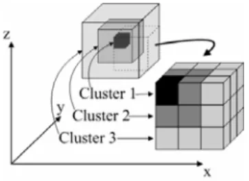
Under the network architecture described in section 3.1, we propose 3D gradient data map to describe the monitored environment. As mentioned above, the sensor nodes are deployed in a 3D space in the monitoring area and each sensor is responsible for sensing the environmental data within its unit cubic cell (We assume that the data within a unit cube have the similar values). Thus, we can aggregate the cubic cells with similar sensor readings into a cube cluster and construct the gradient data map at each sampling period within the network. The gradient data map consists of dif-ferent clusters with their own geometric shapes and data distributions. The gradient data map is an approximation of monitored environment and reflects environmental data dis-tribution at each sampling period.
Fig. 2. 3D space gradient data map
We employ data aggregation in each sampling process and create partial gradient data maps from sensor readings. The partial data maps are merged as much as possible along the paths from sensors to the sink. At the sink, the gradient data map is built from a set of partial gradient data maps. Along with a sequence of sampling, a time series of approximated 3D gradient data maps is constructed at the sink, on which event detection is performed. Figure 2 exhibits a partial gra-dient data map including 3 different cube clusters. We can simply use the average value of all sensor readings in the cube
cluster to approximate the data of this cluster during the aggregation. However, that approach introduces large ap-proximating errors. In our gradient data map, we compute the data distribution f of each cube cluster and describe it with a geometric representation, space orthogonal polyhedra (OP). By manipulating the two parameters of OP, which can be simply transmitted with little bandwidth, the sensor nodes are collaborated to construct the gradient data map in an in-network manner. The key operations in the aggregation process are estimating the similarity of different OPs and merging the similar OPs at each sensor node.
3.3 Space OP Model and Map Construction
We use the space Orthogonal Polyhedra (OP) model to describe different cube clusters. OP can capture the data distribution in 3D cubic space and only requires few pa-rameter settings. The OP was first introduced in Constructive Solid Geometry (CSG). Aguilera and Ayala investigated the characteristics of OP [2] and presented the geometric models to represent OP as well as some basic geometric operations, which are summarized as follows.Definition 3.1:Orthogonal Polyhedra (OP) are polyhedra with all faces oriented in three orthogonal directions.
In an OP, all planes and lines are parallel to three or-thogonal axes. The number of incident edges for each vertex can be only three, four or six, which is referred as V3, V4 or V6, respectively [2]. An Extreme Vertices model (EV model) has been proposed to represent OP.
Definition 3.2:The EV model for OP is defined as a model that only stores all V3 vertices.
Aguilera and Ayala proved that the EV model is a valid
B-Rep model, i.e., it is complete and compact in the sense of geometry. Furthermore, they proposed the ABC-sorted EV model which provides computational convenience for geo-metric operations.
Definition 3.3: An ABC-sorted EV model is an EV model where V3 vertices are sorted first by coordinate A, then by B and then by C.
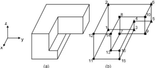
Figure 3 gives an example of the ABC-sorted EV model for the OP. The model is stored as a series of vertices (node 1 to node 16). Based on ABC-sorted EV models, the following geometric operations can be efficiently performed:
1) Volume calculation - To calculate the volume of an OP. An O(n) algorithm exists by accumulating the strip region between any consecutive different sections, where n is the number of vertices of the OP.
2) Relationship checking - To check the relationship of two OPs: overlapping, adjacent or separated. An O(n) algorithm exists by sequentially checking the relationship of the sec-tions of the two OPs along some axis.
3) Boolean operations - To compute the union or intersec-tion or difference of two OPs. An O(n) algorithm exists by sequentially exerting Boolean operations on the sections of the two OP along some axis.
Fig. 3. (a) A hidden line representation of an OP; (b) The order number of its XYZ-sorted EV model.
Fig. 4. The possible relationships of two OP _______________________________________________
Algorithm 1 Partial Map Generating
Input: the active set Sp
Output: the resulting map Mf
1: construct an empty min-heap H, to contain the mergers; 2: for each OP pair OPi and OPj (i ≠ j) in Sp do
3: ifcheckMergeable(OPi , OPj)
4: H. add(createMerger(OPi , OPj ));
5: while not H. empty() do
6: merger m<OP1, OP2> = H. extract();
7: create OP = merge(OP1,OP2);
8: for any merger m containing OP1 or OP2do
9: H. delete(m); 10: Sp. delete(OP1); 11: Sp. delete(OP2); 12: for each OPkin Spdo 13: ifcheckMergeable(OP, OPk ) 14: H. add(createMerger(OP, OPk)); 15: Sp. add(OP);
16: for each overlapping region R=OPi∩OPj in Spdo
17: OPi= OPi− R or OPj= OPj− R;
18: returnMf =Sp;
_______________________________________________ Since a cube cluster is composed of multiple cubic cells, the geometric shape of clusters can be well modeled by an OP which is described by the geometric shape of the covered area and a data distribution function in this area. The partial gra-dient data map stored in each sensor node is represented as a list of OPs depicted by the ABC-sorted EV model. The in-network construction of the gradient data map starts from each node sensing its environment and generating the OP model for its own cell. Each node receives the partial maps from all its child neighbors at the time slot of data aggregation. The OPs from different partial maps form an active set Sp. Through investigating the relationship among OPs within Sp, the sensor node estimates the similarity of OPs and merges the mergeable OPs. Figure 4 illustrates the possible
rela-tionships of two OPs. Finally, the partial maps are aggregated into a single map Mf which includes disjointed OPs. The lower level sensor node transfers Mf to its parent neighbors. Algorithm 1 presents detail steps of partial map generation for each sensor node.
3.4 Aggregation Criteria
To aggregate different partial maps, we need effective criteria to measure the similarity of OPs so that the resulting partial data map well approximates the actual data map.
The OP model used in our system represents a cluster of cubic cells with similar environmental data. We can use a specific data value to represent the data in the whole OP region, e.g., the average value of all the sensor readings in the OP. In such case, to check the similarity of two OPs, we only need check the representing values of them. However, a single data value can hardly reflect full-scale environmental conditions in the OP. Moreover, only investigating the rep-resentative value of an OP will miss the important spatial information. For example, with the same value, an OP oc-cupying a larger space is still different from an OP holding a smaller space. Thus, we can merge a tiny OP (OP with small space) into a much larger OP (OP with large space) even though their representative data values differ a lot, because the merging simplifies the data map representation without losing much accuracy. However for the case in which two OPs both occupy large spaces, merging them may greatly reduce the accuracy of the resulting gradient data map.
In our design, each OP is associated with a data distribu-tion model which describes the environmental data within this OP. A function v = f(x, y, z) is employed to approximate the data value in each spot in the OP, where x, y and z cor-respond to the spot coordinate in the 3D space. Polynomial models can be utilized to formulate this approximation function. To reduce the computational overhead for resource constraint sensor nodes, we adopt the linear model f(x, y, z) = c0 + c1x + c2y + c3z, where the data distribution is approxi-mated by a hyperplane in the 4 dimensional space built on <x, y, z, v>. In the sampling period, each node first computes its initial model for its cubic cell from its sensing reading. During the aggregation, a linear model is built by conducting linear regression (LR) over the whole OP area. For an OP containing n cubes, n values are extracted for all cubes. Thus, we can get n 4-tuples <x1, y1, z1, v1>, <x2, y2, z2, v2>, … , <xn,
yn, zn, vn> from which we compute the coefficients of the linear model by solving the equation: Aw = b
1 1 1 1 0 2 1 1 1 1 1 1 2 2 1 1 1 1 3 1 2 1 1 1 1 1 , , n n n n i i i i i i i i n n n n n i i i i i i i i i i i i i n n n n n i i i i i i i i i i i i i n n n n i i i i i i i i i i x y z v c x x x y x z v x c A w b c y x y y y z v y c z x z y z z = = = = = = = = = = = = = = = = = = ⎛ ⎞ ⎜ ⎟ ⎜ ⎟ ⎛ ⎞ ⎜ ⎟ ⎜ ⎟ ⎜ ⎟ ⎜ ⎟ ⎜ ⎟ = = = ⎜ ⎟ ⎜ ⎟ ⎜ ⎟ ⎜ ⎟ ⎝ ⎠ ⎜ ⎟ ⎜ ⎟ ⎜ ⎟ ⎝ ⎠
∑
∑
∑
∑
∑
∑
∑
∑
∑
∑
∑
∑
∑
∑
∑
∑
∑
∑
1 . (1) n i i i v z = ⎛ ⎞ ⎜ ⎟ ⎜ ⎟ ⎜ ⎟ ⎜ ⎟ ⎜ ⎟ ⎜ ⎟ ⎜ ⎟ ⎜ ⎟ ⎜ ⎟ ⎜ ⎟ ⎝∑
⎠_______________________________________________
Algorithm 2 Merging Manipulations
Function checkMergeable(OPi , OPj)
1: ifOPiand OPj are overlapping or adjacent
2: compute εij;
3: ifεij ≤ε
4: returnTRUE;
FunctioncreateMerger(OPi , OPj )
1: φij = volume(OPi) + volume(OPj) – volume(OPi∪ OPj);
2: ifφij > 0
3: return merger<OP1,OP2> with key εij/φij;
Functionmerge(OP1,OP2)
1: compute OP = OPi∪ OPj;
2: A = Ai + Aj; 3: b = bi + bj;
4: compute w by Aw = b;
5: returnOP with A, b and w;
_______________________________________________ The parameters A, w and b of LR model are integrated and transmitted with the OP in the aggregation process, which take O(1)cost to represent the data distribution over the OP. When merging two OPs, OPi and OPj, we can compute the LR model of the resulting OPij from the LR models of OPi and OPj. By summing Aiand Aj, we get Aij,sodoes bij with respect to bi and bj. The coefficients wij can be derived from the generated Aij and bij. Therefore, we do not need sample the <x, y, z, v> tuples to construct our LR model which is less accurate and induces more overhead. The similarity of two OPs is estimated based on the linear models of OPs. An estimated error bound εij is computed when aggregating two different OPs by the following formula:
(1 ) (1 ) (2) i i j j ij i j R R ε ε ε = + ∆ + + ∆ +
where ∆i represents the difference between the cumulates of fij and fi on OPi, and ∆j represents the difference between the cumulates of fij and fj on OPj:
(
)
(
)
(
)
(
)
(
)
(
)
| , , , , | | , , , , | (3) i j i ij i OP j ij j OP f x y z f x y z d f x y z f x y z d δ δ ∆ = − ∆ = −∫∫∫
∫∫∫
εi and εj are the error bounds for fi on OPi and fj on OPj. Thus, (1+εi)∆i + (1+εj)∆j gives the maximum difference when we substitute the former LR models on OPi and OPj with the aggregated one. Ri and Rj represent the cumulates of fi on OPi and fj on OPj, respectively.
(
, ,)
,(
, ,)
(4)i j
i i j j
OP OP
R =
∫∫∫
f x y z dδ R =∫∫∫
f x y z dδThis formula computes the error bound εij after the ag-gregation, and it is then evaluated by a user defined error bound ε. Only when εij is not greater than ε, two OPs are mergeable. Note that, in the above formula, the error bound is computed in a weighted manner, where the OP volume is the weight factor.
Based on the estimation of the LR model, we consider the
data value as well as the volume of the OP when merging two different OP regions. Algorithm 2 describes the function checkMergeable and createMerger which estimate the simi-larity of two OPs and calculate the key value of the merger. The function merge merges two OPs and computes the new LR model for the resulting OP. The traffic overhead could be further reduced by incrementally updating the data map when sensor readings change.
4.
E
VENTD
ETECTIONWhen the sink receives the aggregated data map, we can perform the event detection based on the exhibited data tern from the data map. Moreover, the spatio-temporal pat-tern revealed from the series of data maps provides us the dynamic progress of the event, which helps capture the event developments. In this section, we describe the event feature patterns and propose a formal method of utilizing the prede-fined feature patterns to detect a specific event.
In previous discussions the term “data map” refers to the constructed gradient data map in some sampling period. For the purpose of event detection, the spatio-temporal data pattern is often investigated over a time series of data maps. For the convenience of description, without specification, we will later use “data map” referring to the spatio-temporal data map consisting of a time series of received data maps. Each data map in this series is referred as a data map “snapshot”.
4.1 Event Feature Patterns
The event feature pattern F is defined as a time series of snapshots L on the data map of some environmental attribute and a set of relationship R among them. L = {S0, S1, …, Sn}, where Si is a snapshot (ti, Mi) on the data map composed of the time label ti and current data map Mi. Here ∆t = ti+1 – ti is the sampling interval between two consecutive snapshots and the data map Mi consists of different OPs (Pi1, Pi2, …, Pim). Different OPs are associated with different data values vij. The relationship R specifies the event feature pattern on series L. R describes the spatial relationship RS by regulating the relationships R(Pik, Pil) between different OPs on the data map snapshot Mi and the temporal relationship RT by regu-lating the relationships R(Mi, Mj) between different data map snapshots. We illustrate the feature pattern in detail by de-scribing two example events and their feature patterns. Spreading Event
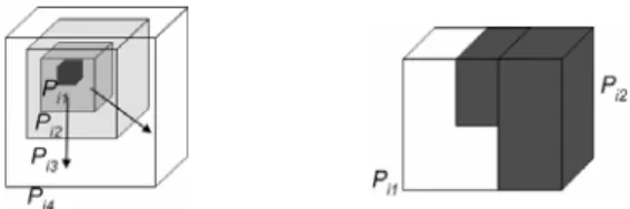
For the event of gas leakage, as the gas spreads from the source spot, the distribution of the gas density follows the single source spreading model in the data map of gas density. Spatially, in the data map snapshots, the leakage source bears the highest gas density value and the value falls along all directions from the source spot. Temporally, as time passes, the abnormal region expands and the gas density rises within the whole region. According to above observed features, we specify the spreading event feature pattern as follows.
The spreading event feature pattern Fs is determined by the user specified snapshot series Ls and the relationship Rs on
them, which are customized by the users: (1) T is a user specified event duration, which constrains that in the snap-shot series Ls, the time interval between the first snapshot S0 and last snapshot Sn, tn – t0 = T. (2) The spatial relationship RSsregulates a series of nesting OPs {Pi1, Pi2, …, PiNi} for each Mi. Ni (0 ≤ i ≤ n) is the user specified spreading level, which specifies the number of the nesting OPs. Pik occupies the hole region in Pik+1. The difference of data values asso-ciated with the two OPs vik − vik+1 is bounded by the user specified degrading bound [DL, DH] and the ratio of their volumes δk/δk+1 is bounded by the user specified scaling bound [fL, fH], (0 < fL < fH < 1). (3) For the temporal rela-tionship RTs, the variation of data values between two con-secutive data maps Mi and Mi+1 is regulated by the user specified variation factor vf,such that the data value variation for any spot p in the event region between Mi and Mi+1, vpi −
vpi+1 ≥ vf. Another user specified spreading factor sf (0 < sf < 1) constrains the ratio of the volumes of event regions (composed of the nesting OPs) in consecutive data maps Mi and Mi+1, such that Ei/Ei+1 ≤ sf. This factor indicates the spreading speed of the source. Figure 5 (a) illustrates the spreading event.
Fault Event
The fault event corresponds to those breaking out changes in terms of some attribute value. For instance, the under-ground water seepage on the tunnel floor induces a large flooded region where the sensory readings largely differ from those in the normal region. The feature pattern of fault event is specified as follows.
The fault event feature pattern Ff is determined by the user specified snapshot series Lf and the relationship Rf on them, which are customized by the users: (1) T is a user specified event duration, which constrains that in the snapshot series Lf, the time interval between the first snapshot S0 and last snapshot Sn, tn – t0 = T. (2) The spatial relationship RSf regulates two adjacent OPs, Pi1 and Pi2 in each Mi. Pi1 is associated with value vi1 in the range [b1, b1+k] and Pi2 with value vi2 in the range [b2, b2+k]. b2 − b1 ≥∆, where ∆ is a user specified threshold. The volumes of the two OPs E1, E2 ≥ E, where E > 0 is a user specified region size bound. Another user specified parameter Sc sets the lower bound of the co-incident plane area shared by the two OPs. (3) The temporal relationship RTf regulates the event regions in consecutive data maps overlap at least at a percentage of α, where 0 <α < 1 is a user specified confidence factor. Figure 5 (b) illustrates the fault event.
Fig. 5. Illustration of example event feature patterns. (a) Spreading event pattern, and (b) Fault event pattern
4.2 Pattern Based Event Detection
Once the event feature patterns have been specified, the sink continuously processes the received data maps and compares them with those predefined event feature patterns. Once finding a match between the pattern and the data map, the corresponding event is captured. More over, by tracking the spatio-temporal feature of the data map series, the de-velopment of current event could also be revealed.
We define an instant snapshot At of the data map A matches Si if and only if the OPs in At match the OPs in Mi and share the same spatial relationships R(Pik, Pil). We define the data map A matches pattern F if and only if from time t, there exist a series of map snapshots {At, At+∆t1, …, At+n∆t} from A, such that any snapshot At+i∆t matches the corresponding feature snapshot Si and all map snapshots obey the temporal rela-tionships R(At+i∆t, At+j∆t).
5.
P
ERFORMANCEE
VALUATIONWe conducted a field study by investigating the various environmental conditions in the D. L. Coal mine. It is one of the most automated coal mines worldwide. We collected different sets of real data in the field and from historic records under normal and exceptional situations. In this section, we investigate the efficacy and efficiency of our proposed event detection mechanism by a trace driven simulation using synthetic workload generated from the collected raw data.
5.1 Simulation Setup
We simulated the event scenarios in a sensor network with a 3D sensor deployment. The widely used Mica2 motes [7] are presumed as the underlying hardware standard. All numbers are 2-byte integers (including sensor readings and all coefficients). The size limit for the simulated packets is set to 60 bytes. An N × N × N cubical grid topology is initiated with a sensor node placed at the center of each cubical grid. The parameter N indicates the diameter of this cubical grid network, ranging from 5 to 20 (default value is 10) in our experiments to explore the system scalability under different network sizes. Each sensor node has direct communication links with 6 surrounding neighbor nodes. The link quality is measured with the link loss rate q, which is the probability that a packet transmitted along the link gets lost. In our ex-periment, this parameter varies from 0% to 40% (default value is 10%) to explore the system reliability under different network conditions.
Three types of real-world historic sensory data for the underground environment have been collected in the coal mine as our data trace including gas density, oxygen density, and watery regions. However, due to the constraint on re-source and environment, the original data are collected with rough granularity on time scale and incomplete samples on the space scale. Based on the raw data on hand, we generate more detailed synthetic datasets for use in our experiment.
0 10 20 30 40 0 20 40 60 80 100 link quality (%) re ca ll ( % ) AGG SAM SAT 5 10 15 20 0 20 40 60 80 100 network diameter re ca ll ( % ) AGG SAM SAT 40 30 20 10 0 20 40 60 80 100 event frequency (%) re ca ll ( % ) AGG SAM SAT (a) (b) (c) Fig. 6. Event detection recall of three approaches with different parameters varying. (a) link quality; (b) network diameter.
(c) event frequency 0 10 20 30 40 0 5 10 15 20 25 30 link quality (%) tra ffic ove rh ead (M B ) SAM SAT AGG 5 10 15 20 0 40 80 120 160 200 network diameter tra ffic ov er he ad (M B ) SAM SAT AGG 40 30 20 10 0 0 5 10 15 20 25 30 event frequency (%) tra ffi c ov er he ad (M B ) SAM SAT AGG (a) (b) (c) Fig. 7. Network traffic overhead of three approaches with different parameters varying. (a) link quality. (b) network
diameter. (c) event frequency
The events are queried over the dataset with a predeter-mined event frequency f, which depicts the monitoring workload. f is calculated as the duration of events over the total monitoring duration. In our experiment, we vary f from 0% to 40% (default value is 10%) to obtain a full view of the system efficiency under different workload.
We focus on two metrics for performance evaluation. The event detection accuracy measures the efficacy of the ap-proach and the network traffic overhead tells the efficiency on energy consumption. The event detection accuracy is measured by two sub-metrics, precision and recall, which have been widely used in IR domain [3]. The precision de-scribes the detection precision, which is defined as the per-centage of accurately detected real events over all reported events; recall describes the detection completeness, which is defined as the percentage of successfully detected events over all occurred events. The network traffic overhead is meas-ured by the total amount of messages (bytes) transmitted in the network in the monitoring duration.
To evaluate the performance gain of our approach, we did a comparative study investigating three possible approaches: (1) AGG: our proposed in-network data map aggregation approach described in section 3. (2) SAT: the server side aggregation under TAG [12] framework, in which the net-work is organized into tree structure and all data are for-warded to the sink. Data map is constructed in the server side. (3) SAM: the server side aggregation under multi-path rout-ing strategy [14], in which the network is organized into
multi-path routing style and the data map is constructed in the server side.
5.2 Simulation Results
We evaluate the performance of event detection accuracy by two metrics: precision and recall. However, since in all runs of experiments, 100% detection precision is consistently achieved in different approaches under all parameter settings, we omit this metric and only present the performance on recall in the experiment result part.
We do the comparative study among the three approaches under various parameter settings. Figure 6 plots the event detection recall of three approaches. In all cases, our AGG approach achieves best performance. As shown in Fig. 6(a), with the increase of the link loss rate, the recall of SAT ridly drops below 40% and tends to 0. While the SAM ap-proach also bears a bad detection recall, our AGG apap-proach demonstrates good tolerability to the network quality. The detection recall is kept above 60% even in a lossy network with up to 40% link loss rate. In Fig. 6(b), the network di-ameter is enlarged to investigate the scalability of three ap-proaches. Again, the SAT approach leads to unacceptable detection recall rate. Our AGG approach keeps high recall rate all along while the recall of SAM approach drops linearly as the network diameter increases. Figure 6(c) plots the de-tection recall of three approaches in cases with different event frequencies. We observe that the parameter of event fre-quency hardly influences the recall rate of the three
ap-proaches. All three approaches provide stable recall rates when event frequency is varied and our AGG approach outperforms the other two.
Figure 7 plots the network traffic overhead in three ap-proaches. In Fig. 7(a), with the increase of the link loss rate, the traffic overhead of all three approaches decreases because of the loss of packets. The SAM approach experiences a faster decrease on the traffic overhead, but the total amount is much larger than the SAT and our AGG approaches. The traffic overhead of the SAT approach has a skip decrease when the link loss rate changes from 0% to 10%, however from Fig. 6(a) we know this is because most of the useful information gets lost due to the packet loss. Figure 7(b) shows how network traffic overhead grows as the network size increases. We note that while the SAT and AGG approaches maintain comparative low traffic overhead against the in-crease of network diameter, the SAM approach has a dra-matic increase of the traffic overhead which greatly con-strains its scalability. Figure 7(c) shows how the parameter of event frequency affects the three approaches. While the event frequency has little influence on SAM and SAT approaches, the traffic overhead of our AGG approach is reduced as the event frequency decreases benefiting from the data map updating technique. According to our autoptical investigation in the coal mine, generally the event frequency in the real-world remains low, benefiting the application of our AGG approach.
To summarize, among the three possible approaches, the SAT approaches introduces the least traffic overhead, but provides the worst, totally unacceptable event detection accuracy; the SAM approaches provides somewhat tolerable event detection accuracy, but with the most traffic overhead and the worst scalability; our AGG approach provides the best event detection performance with relatively small traffic overhead. We also achieve the best scalability to the network size and tolerability to the network quality in the AGG ap-proach.
6.
C
ONCLUSIONS ANDF
UTURE WORKIn this paper, we propose a non-threshold based approach for complex event detection in 3D environment monitoring applications. Other than threshold based approaches, we propose event feature patterns to specify complex events and develop a pattern based event detection method on the ob-tained 3D gradient data map. We employ multi-path routing architectures to provide robust data delivery and perform in-network aggregation on it to efficiently construct the data map. Space OP model is proposed to describe the environ-ment data distributions. Partial data maps are aggregated by merging OP regions with similar environmental data. Our experimental results show the performance gain of our en-ergy-efficient techniques. Moreover, the comparative study with two alternative approaches exhibits that our approach achieves great event detection accuracy with small network
traffic overhead.
The future work includes implementing a working system in real-world environment. To carry on pattern recognition on the obtained gradient data maps with machine learning techniques on historic data samples may provide more effi-cient detection methods, which will also be included in our future work.
A
CKNOWLEDGEMENTThis work is supported in part by the Hong Kong RGC grant HKUST6152/06E and DAG05/06.EG03, the HKUST Digital Life Research Center Grant, the National Basic Re-search Program of China (973 Program) under grant No. 2006CB303000, and NSFC Key Project grant No. 60533110.
R
EFERENCES[1] D. Abadi, S. Madden and W. Lindner, "REED: Robust, Effi-cient Filtering and Event Detection in Sensor Networks," in Proceedings of VLDB, 2005.
[2] A. Aguilera and D. Ayala, "Orthogonal Polyhedra as Geo-metric Bounds in Constructive Solid Geometry," in Proceed-ings of Solid and Physical Modeling Symposium, 1997. [3] R. Baeza-Yates and R. N. Berthier, Modern Information
Re-trieval: Addison-Wesley, 1999.
[4] P. Bonnet, J. Gehrke and P. Seshadri, "Querying the physical world," IEEE Personal Communications, vol. 7, 2000. [5] R. Burns, A. Terzis and M. Franklin, "Design Tools for
Sen-sor-Based Science," in Proceedings of EmNets, 2006. [6] J. M. Hellerstein, W. Hong, S. Madden and K. Stanek,
"Be-yond Average: Toward Sophisticated Sensing with Queries," in Proceedings of IPSN, 2003.
[7] J. Hill and D. Culler, "Mica: A Wireless Platform For Deeply Embedded Networks," IEEE Micro, vol. 22, pp. 12 - 24, 2002. [8] C. Intanagonwiwat, R. Govindan and D. Estrin, "Directed
Diffusion: A Scalable and Robust Communication Paradigm for Sensor Networks," in Proceedings of ACM MobiCom, 2000.
[9] S. Li, Y. Lin, S. Son, J. Stankovic and Y. Wei, "Event detec-tion services using data service middleware in distributed sensor networks," Telecommunication Systems, vol. 26, 2004. [10] Z. Li and B. Li, "Loss Inference in Wireless Sensor Networks based on Data Aggregation," in Proceedings of IPSN, 2004. [11] S. Lindsey, C. Raghavendra and K. Sivalingam, "Data
Gath-ering in Sensor Networks using Energy Delay Metric," in Proceedings of IPDPS, 2001.
[12] S. Madden, M. J. Franklin and J. M. Hellerstein, "TAG: a Tiny AGgregation Service for Ad-Hoc Sensor Networks," in Pro-ceedings of OSDI, 2002.
[13] V. Mhatre, C. Rosenberg, D. Kofman, R. Mazumdar and N. B. Shroff, "Design of Surveillance Sensor Grids with a Lifetime Constraint," in Proceedings of EWSN, 2004.
[14] S. Nath, P. B. Gibbons, S. Seshan and Z. R. Anderson, "Synopsis diffusion for robust aggregation in sensor net-works," in Proceedings of ACM SenSys, 2004.
[15] I. Solis and K. Obraczka, "Efficient Continuous Mapping in Sensor Networks Using Isolines," in Proceedings of IEEE Mobiquitous, 2005.