A case study: Failure prediction in a real LTE network

(1)

ANOMALY

DETECTION

IN

SELF-ORGANIZING

NETWORK

A case study: Failure prediction in a real LTE network

Master’s Thesis

Viet Nguyen

Aalto University School of Business

Information and Service Management

Fall 2019

(2)

(3)

Abstract of master’s thesis

i Author Viet Nguyen

Title of thesis ANOMALY DETECTION IN SELF-ORGANIZING NETWORK Degree Master of Science in Economics and Business Administration

Degree programme Information and Service Management Thesis advisor(s) Prof. Tomi Seppälä

Year of approval 2019 Number of pages 51 Language English Abstract

Mobile traffic and number of connected devices have been increasing exponentially nowadays, with customer expectation from mobile operators in term of quality and reliability is higher and higher. This places pressure on operators to invest as well as to operate their growing infrastructures. As such, telecom network management becomes an essential problem. To reduce cost and maintain network performance, operators need to bring more automation and intelligence into their management system.

Self-Organizing Networks function (SON) is an automation technology aiming to maximize performance in mobility networks by bringing autonomous adaptability and reducing human intervention in network management and operations. Three main areas of SON include configuration (auto-configuration when new element enter the network), self-optimization (self-optimization of the network parameters during operation) and self-healing (maintenance).

The main purpose of the thesis is to illustrate how anomaly detection methods can be applied to SON functions, in particularly self-healing functions such as fault detection and cell outage management. The thesis is illustrated by a case study, in which the anomalies - in this case the failure alarms, are predicted in advance using performance measurement data (PM data) collected from a real LTE network within a certain timeframe. Failures prediction or anomalies detection can help reduce cost and maintenance time in mobile network base stations. The author aims to answer the research questions: what anomaly detection models could detect the anomalies in advance, and what type of anomalies can be well-detected using those models.

Using cross-validation, the thesis shows that random forest method is the best performing model out of the chosen ones, with F1-score of 0.58, 0.96 and 0.52 for the anomalies: Failure in Optical Interface, Temperature alarm, and VSWR minor alarm respectively. Those are also the anomalies can be well-detected by the model.

(4)

Maisterintutkinnon tutkielman tiivistelmä

ii Tekijä Viet Nguyen

Työn nimi ANOMALY DETECTION IN SELF-ORGANIZING NETWORK Tutkinto Master of Science in Economics and Business Administration Koulutusohjelma Information and Service Management

Työn ohjaaja(t) Prof. Tomi Seppälä

Hyväksymisvuosi 2019 Sivumäärä 51 Kieli Kieli Tiivistelmä

Mobile traffic and number of connected devices have been increasing exponentially nowadays, with customer expectation from mobile operators in term of quality and reliability is higher and higher. This places pressure on operators to invest as well as to operate their growing infrastructures. As such, telecom network management becomes an essential problem. To reduce cost and maintain network performance, operators need to bring more automation and intelligence into their management system.

Self-Organizing Networks function (SON) is an automation technology aiming to maximize performance in mobility networks by bringing autonomous adaptability and reducing human intervention in network management and operations. Three main areas of SON include configuration (auto-configuration when new element enter the network), self-optimization (self-optimization of the network parameters during operation) and self-healing (maintenance).

The main purpose of the thesis is to illustrate how anomaly detection methods can be applied to SON functions, in particularly self-healing functions such as fault detection and cell outage management. The thesis is illustrated by a case study, in which the anomalies - in this case the failure alarms, are predicted in advance using performance measurement data (PM data) collected from a real LTE network within a certain timeframe. Failures prediction or anomalies detection can help reduce cost and maintenance time in mobile network base stations. The author aims to answer the research questions: what anomaly detection models could detect the anomalies in advance, and what type of anomalies can be well-detected using those models.

Using cross-validation, the thesis shows that random forest method is the best performing model out of the chosen ones, with F1-score of 0.58, 0.96 and 0.52 for the anomalies: Failure in Optical Interface, Temperature alarm, and VSWR minor alarm respectively. Those are also the anomalies can be well-detected by the model.

(5)

iii

List of Tables

Table 3-1 Confusion matrix ... 20

Table 4-1 List of predictors ... 23

Table 4-2 Feature importance of random forest ... 39

List of Figures

Figure 2-1 Mobile network with cellular design ... 4

Figure 2-2 SONs function and major uses cases ... 7

Figure 3-1 CRISP-DM process ... 13

Figure 3-2 Example of Decision tree design ... 16

Figure 3-3 Example Random Forest model architecture ... 17

Figure 3-4 Example of a simple multilayer-perceptron architecture ... 19

Figure 4-1 Distribution of number of alarms per base station ... 26

Figure 4-2 Number of alarms occur at each hour of the day ... 27

Figure 4-3 Number of alarm hour by hour ... 27

Figure 4-4 Distribution of number of timestamps in each base station ... 28

Figure 4-5 Scaled KPIs and Alarm data from a specific base station ... 29

Figure 4-6 Correlation matrix of scaled KPIs in a specific base station ... 30

Figure 4-7 Effect of different pre-processing techniques to address imbalance data on the evaluation benchmark ... 32

Figure 4-8 Effect of different dimension reduction techniques on the evaluation benchmark ... 33

Figure 4-9 Number of failure alarms across different time-series cross validation folds ... 34

Figure 4-10 Comparison of different models on validation sets with different target features ... 36

Figure 4-11 Different hyperparameter settings of Random Forest with different target features ... 37

Figure 4-12 Evaluation benchmark of Random Forest on testing sets with different target features ... 38

Figure 4-13 Confusion matrix of Random Forest models on different target features ... 39

(8)

1 Introduction

1.1 Background and motivation

1.1.1 Background

Mobile traffic and number of connected devices have been increasing exponentially nowadays, with customer expectation from mobile operators in term of quality and reliability is higher and higher. This places pressure on operators to invest as well as to operate their growing infrastructures. Several breakthrough technologies have been discussed in the literature over the past few years in telecom network management, one of them is the implementation of Self Organizing Networks function (SON)

SON is an automation technology aiming to maximize performance in mobility networks by bringing autonomous adaptability and reducing human intervention in network management and operations. SON is designed to be able to improve itself via constant interaction with the network environment and also its action consequences. Three main areas of SON include self-configuration (auto-configuration when new element enter the network), optimization (optimize the network parameters during operation) and self-healing (maintenance).

In practice, most operators still employ rudimentary methods to configure, optimize and maintain the network operation performance. For example, the configuration of thousands base stations (BS) parameters is done manually by experienced radiologists. Telecom expert personnel are also needed to manually analyze measurement reports to continuously optimize the network. In regard to network maintenance, human experts are also required to monitor the failure alarms and manually adjust the system parameters to correct the failures. Operators also have to perform periodic drive tests every once in a while in order to test and optimize the network performance. With the growing scale of infrastructure, such practices become increasingly costly and ineffective, results in the need for a comprehensive automation solution in telecom network management.

One of the functionalities of SON that gains most attraction from operators is self-healing. Self-healing means to maintain the resources so that LTE base station (can also be referred as cell, node throughout this thesis) can work normally according to customer expectation, or specifically, minimize the time when any base station fails to work normally (i.e. downtime). Downtime can occur due to internal and external reasons, from old hardware components to weather conditions like lightning strikes or solar radiation. When failures

(9)

occur, it must be recognized and notified to the network operator. The operator can fix the failures in multiple ways, either dispatching its maintenance crew to replace the old hardware or simply do a system reset. However, solving the problem this way still requires time, and operators are interested in cutting down such downtime even more by looking at more active solutions. (Elisa Oyj.; Enne Analytics Inc., 2018)

1.1.2 Motivation

The primary motivation of this thesis comes from a challenge faced by a case company. The case company is Elisa, one of the biggest telecom operators in Finland. Its current mission is to create a SON solution, i.e. an automation solution of telecom management for itself and all other operators over the world. One of the challenges is anomaly detection – to detect/predict abnormal network behavior in cellular systems. The problem belongs to self-healing category in SON context.

This thesis will focus specifically on detecting and predicting cell failure, one of the abnormal network behaviors. Successfully detection and prediction in advance are important in many perspectives. Failures can be repaired in a more timely and active manner, leading to reduced downtime and more satisfying experience for customers.

1.2 Research problem

As mentioned above, this thesis aims at solving the problem of detecting the anomaly (i.e. failure prediction) in telecom network, in order to help minimize downtime and reduce operating cost. The primary research problem will be:

How anomaly detection models can be applied on telecom network performance data to detect in advance the anomalies or failures in the mobile network?

1.3 Aim of the study

The use of machine learning model, specifically anomaly detection algorithm in the field of telecommunication network management is not entirely new. Various earlier studies on the same topic will be discussed in the literature review. However, as telecom management is a broad field with many specific use-cases, most of the studies focus on different uses-cases than the case in this thesis and produces inconsistent results with varying degree of success. Moreover, most of the studies in literature only used simulated data, as real telecom data is difficult to obtain and access. Therefore, it is still a question whether real data in practice

(10)

can lead to different results. This thesis uses real data in order to verify the applicability of the models, whether or not those models can produce consistent results.

In addition to the main objective, this thesis can also serve as an intermediary between existing anomaly detection literature and its application in SON network. As such, the thesis can also provide a good literature source for further research in the field.

To put it clearly, the thesis aims to answer the following research questions:

Could these anomaly detection algorithms be applied to case company data to detect anomalies in advance?

1. What models give the best predictive performance?

2. What types of anomalies can be well-predicted using those models?

1.4 Structure of the Thesis

The thesis starts with the research question statement and its motivation. Chapter 2 provides a summary of literature review of relevant topics. Chapter 3 provides the main framework based on which the whole machine learning project is carried out. Chapter 4 shows how the framework is implemented and how the answer to research question is provided. Chapters 5 and 6 are concluding chapters, providing the insights obtained from the theory and practical experiments and laying out the limitations, future work, and contributions of this thesis.

(11)

2 Literature review

2.1 Application domain: Self-organizing network (SON)

As mobile traffic demands become higher, operators also have their infrastructure growing on a bigger scale in order to afford those demand. Therefore, management and operations of telecom networks become more important in maintaining the reliability, quality and dependability of the networks (Subramanian, 2000)

2.1.1 Mobile network overview

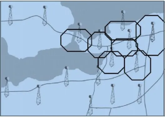
Mobile networks are often referred as cellular network because the networks are divided into smaller land areas called cells, each served by one or more Base Transceiver Stations (BTS). Each BTS provides coverage to a certain area. BTS are placed at planned locations so that the whole cellular network is able to provide continuous coverage to all customers. Figure 2-1 shows how part of a mobile network is divided into multiple cells, in which located by a BTS.

Figure 2-1 Mobile network with cellular design

When a customer makes a call, a radio connection is created from the caller to the BTS that serving his current area. The call is received by the BTS and then transmitted throughout the network to its destination (Pautet, 1992)

(12)

2.1.2 Mobile network management

As demand increases, it becomes more complex to maintain the performance as well as quality of service of the telecommunication network. Thus, network management is important, and gains substantially interest from operators. The purpose of network management is to maximize the capacity of a telecommunication network (Freeman, 2004). For example, network management should be able to secure peak performance of different network components, to notice the operator of any degradation, and to diagnose failures using fault diagnosing tools and so on.

Network operators often rely on a computer system called Operation Support Systems (OSS) to manage their network. OSS manages the network by sending out data (such as configuration parameters) to other Network Equipments (NEs), and in return, receiving data (such as performance report, failure report) from NEs.

Telecommunication network management comprises of the following management functionality (Burke, 2003):

• Fault Management: to detect, record, notify network administrators and fix network issues.

• Configuration Management: to monitor the overall network and system configuration and its related information, to track and analyze the impact of various network operations.

• Performance Management: to measure the network performance data and report it back to the network management unit, with the aim to maximize the performance of the network

• Security Management: to control the access to network resources according to organizational security guidelines.

2.1.3 Key Performance Indicators

The purposes of data collection from the telecom network are to support operational control and decisions making, and to acquire knowledge of the application domain. Raw data, or low-level data, often referred as counters, are collected from various operational activities of the network. Depending on management purposes, the time frames for the counting purposes could be varying. Low-level data are often combined together by certain formulas to form more understandable and interpretable counter variables, often called Key Performance Indicators (Suutarinen)

(13)

Each operator has its own way to define and its own formulas to compute these KPIs, even two KPIs with the same name but from different operators are not necessary using the same formulas.

2.1.4 Self-Organizing Networks (SON) and Self-Healing

As mentioned previously, the demand on network increases, the network management becomes increasingly difficult and burdensome. Especially in fault management area, new type of failures emerge on a continuous basis. Human intervention become less and less effective in addressing the problem quickly. This is the reason why framework such as SON comes to existent.

Self-organizing networks (SON) is a telecom management framework aims at automation of network functions and operations. SON is implemented by creating the logic for the whole system using a pre-programmed set of rules and conditions. The logic is then fed into the system, which in turn regulates, control and select appropriate actions for the whole network based on the state of the NEs. The logic of SON should enable it to learn from its interaction with the environment and past action taken by the system. To sum up, SON is designed so that it can be characterized as adaptive and autonomous as well as scalable, stable and agile (O. G. Aliu, 2013)

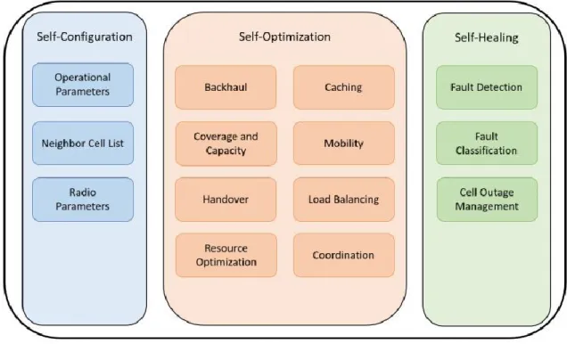
The concept of SON in mobile networks is divided into three main categories: self-configuration, self-optimization and self-healing

• Self-Configuration: refer to the ability of the network to automatically apply necessary configuration procedures during the initial stage of network deployment, such as when there is a change in the network system, or a new base station deployed in the system. Thus, self-configuration also helps to reduce downtime. The configuration parameters include individual Base Station (BS) configuration parameters and configurations that will be applied to the whole network.

• Self-Optimization: as its name implies, self-optimization refers to a group of functionality areas that aim at optimizing the BSs and network parameter to achieve maximum performance as possible. Self-optimization is divided into further sub-areas such as caching, coverage and capacity optimization, backhaul optimization, mobility optimization, antenna parameters optimization, load balancing, resource optimization, Handover (HO) parameters optimization, energy efficiency optimization etc.

• Self-Healing: refer to the ability of the network to detect failures, perform diagnostic analysis on the failures and provide appropriate solutions to fix the failures. Faults and

(14)

failures can occur at any time during operation in any cellular system. Self-healing function aims at establishing reparation mechanism so that the network can make a smooth and fast recovery. Self-healing is divided into smaller sub-areas: fault detection, fault classification and cell outage management (3GPP TS, 2012)

Figure 2-2 SONs function and major uses cases

Also, each SON function can be divided into sub-sections, commonly known as use-cases. As it can be seen from figure 2-2, SON is expected to provide automated solutions to several different use cases and some of which even doesn’t exist today yet but will be important in the future network. SON is believed to be the key important part of future 5G networks, bring the adaptability and flexibility required to implement the network of the future. (Klaine, Imran, Onireti, & Souza, 2017)

In order for SON to meet its expectation, not only automation but also artificial intelligence needs to be employed. Currently, in practice, operators collect a huge amount of mobile data daily, it is not being used at its full potential. With the rising popularity Machine learning (ML) and computing power becoming cheaper and cheaper, it is possible to apply different ML solutions in the collected data in order to explore the potential usefulness of ML in different SON use cases. A future well-functioning SON system is expected to employ some sort of ML and artificial intelligence (Moysen & Giupponi, 2018)

(15)

2.2 Anomaly detection

As its name implies, anomaly detection is the identification of anomalies. Anomaly detection plays an important part in data mining (P.-N. Tan, 2005). From the literature, there are two different understanding of anomalies. Although in some case, there is no distinct separation between these two meanings as both of them refers to the same type of objects, it is still important to distinguish in most cases.

2.2.1 Definition of Anomalies

An anomaly is widely defined as “something that deviates from what is standard, normal or expected” (The Oxford Dictionary of English, Revised Edition, 2005) In other words, it refers to all of the unexpected events, including observed or unobserved. In machine learning and data science literature, anomalies are defined as rare items, events or observations which differ significantly from the majority of the data. They are also called outliers, noise, deviations and exceptions. Anomalies, in this case, receive attention for several reasons. One of them is for the purpose of removing anomalous data from the dataset. For some supervised machine learning model, this often leads to a statistically significant increase in accuracy.

In some specific application domain, anomalies, however, contain different meaning. Particularly, in the context of telecom network, the interesting object could be some abnormal behavior in the network, for example hardware failures. This object is not necessarily rare object as defined from statistical perspective but is considered as rare from the domain application perspective. In this case, many outlier detection methods, especially unsupervised methods, are likely to fail on such data (Aggarwal, 2016). To detect such abnormal behavior is the interest of various stakeholder from multiple domains and industries: fraud detection in financial transaction, event detection in sensor networks. (Kumpulainen, 2014)

This thesis considers anomalies to have the latter meaning – i.e. application specific, or in this case, abnormal event that occurs during the operation of the network. When referring to the first meaning, i.e. data instance that significantly differs from others, the thesis uses the term outliers

In the telecom network domain, anomalies are often termed with various failures could happen in the network such as poor network coverage, cell failures, cell traffic congestion, etc. Within the SON framework, anomaly detection models are used mainly in self-healing to detect abnormal network behavior, especially cell outage detection. In this thesis, anomaly

(16)

detection will be implemented with the case company data to solve the problem of failure prediction. (Klaine, Imran, Onireti, & Souza, 2017)

2.2.2 Anomaly detection methodology

There are many anomaly detection methods, and they are often classified into broader categories based on their characteristics, i.e. how the inner algorithm works and handling the data. Typically, an anomaly detection method could be classified as distribution-based (density-based), proximity-based (distance-based) or cluster-based (M. Agyemang, 2006)

Another way to classify all those algorithms is based on what kind of problem to be solved and what data those algorithms are applied into, namely unsupervised, supervised and semi-supervised.

2.2.2.1 Unsupervised anomaly detection techniques

Unsupervised anomaly detection techniques aim to solve unsupervised problems, in which the dataset is unlabeled with the assumption that the majority of the data are normal. The anomalies are the instances seem to fit least to the rest of the dataset (Zimek & Schubert, 2017)

It is not guaranteed that unsupervised methods could detect the anomaly that is of interest for the domain application. In practice, there are often multiple types of anomaly associated with multiple different activities that could occur in a system. An unsupervised anomaly detection method might discover noise, which is not specific to any of those activities, and thus might not of relevance to the problem (Aggarwal, 2016)

2.2.2.2 Semi-Supervised techniques

Semi-supervised techniques assume the training data contain only normal instances. Typically, all the data points are labeled as normal, and what deviates from those recognized normal is consider anomalous. Being trained on the normal dataset, the constructed model from those techniques will be applied to a test dataset, which could contain both normal and anomalous instances. The anomalous are the ones least likely being generated by the trained model.

2.2.2.3 Supervised techniques

Supervised anomaly detection methods expect input training data to be labeled and to contain both normal and anomalous classes. In this case, the anomaly detection model could be any machine learning classifier, and the problem could be considered as classification problems. However, the key difference is the inherently unbalanced ratio between normal

(17)

and anomalous – the majority of the dataset is normal data. This also poses a challenge to the classifier and additional pre-processing step would be required to achieve certain accuracy performance.

Because of the availability of labeled data, especially labeled anomalous, supervised anomaly detection is able to detect different domain-relevant anomalies. From the literature review, it is always recommended to use supervision as long as possible. It is observed that even a small amount of supervised anomalous data could improve outlier detection accuracy in a significant way (Aggarwal, 2016). Unlike unsupervised methods, supervised techniques can be used to detect multiple anomalies at once, given that labeled data for each anomaly are available.

2.3 Anomaly detection in SON context

Although machine learning solutions have been widely experimented and applied in the context of SON, anomaly detectors have been only employed in the context of self-healing functions, particularly in the cell outage management and fault detection uses cases. (Klaine, Imran, Onireti, & Souza, 2017)

2.3.1 Fault detection

Fault detection refers to the capability of estimating the time and location of a network failure. This also implies the ability to predict in advance whether or not a fault will occur in the network. Fault detection often requires certain KPI or performance measurement data, however, other data sources such as traffic or user mobility-related data are sometimes utilized. There are various studies in the literature that used various anomaly detection and machine learning models for fault detection.

In (G. F. Ciocarlie, 2013), the author used an ensemble method to combine different support-vector machine classifiers to classify the performance status of cells in the network. In (A. Coluccia, 2011), the author also used Bayes’ estimators on several KPIs data to predict when a failure might occur in a simulated mobile network.

Self-organizing map (SOM), an original unsupervised artificial neural network, were also widely used, either directly or indirectly, in several other studies. In (K. Raivio, 2003) the author modified SOM algorithm into a classification algorithm so that it can classify the performance status of cells into several categories, such as acceptable or degraded.

Statistical analysis also provides a tool for anomaly detection. One can detect the anomalies by looking at the statistic distribution of the feature being studied. For example,

(18)

in (A. D’Alconzo, 2009) , D’Alconzo et al, by identifying deviation in traffic data distribution, he created an algorithm that can detect and predict when a failure could happen in the network.

Similarity-based anomaly detection method is also widely used in this case. In this approach, a dissimilarity metric is computed, and data instances are classified based on the metric. For example, in (Olariu, Aug 2009), Bae and Olariu built a normal profile from the pattern of user mobility and used the algorithm on the new data to detect the anomalies.

In addition to KPIs data, other relevant sources of data could also be used to detect abnormal behavior in the network. In (P. Fiadino, 2015) the authors built a real-time dataset from several Domain Name System (DNS) features. Using statistical analysis, the author set up a threshold so that whenever the DNS feature change significantly based on the threshold, a flag is triggerred, signaling that an anomaly might happen. On the other hand, in (A.Gmez-Andrades, 2017), the authors applied SOM clustering method into Minimization of Driving Test (MDT) measurements data in order to detect whenever a fault happens in the network. The proposed method showed that it can detect and locate failures within the network up to a certain degree of accuracy.

In (Stanczak, 2015), Liao et al., combined dimension reduction with local outlier factor – an unsupervised method, in order to detect the anomalies. The dataset’s number of dimensions were reduced using Principle component analysis (PCA). The results are optimistic, with high performance in a simulated LTE network.

2.3.2 Cell outage management

Cell outage is the case when one typical cell ceases to function as expected and go out of service. In a cell outage scenario, operators need to act quickly to correct the problem and minimize its disruption to the overall network. As cellular networks grow faster and larger, it becomes more ineffective for the operators to detect cell outages, especially with their current manual methods. One of the SON self-healing function is cell outage management, which involves the automating detection of cell outage within the cellular network.

Another special case of cell outage is sleeping cell, which is also worthy to mention Technically, a sleeping cell is also a failed cell, providing little to no service to the customers. However, from the operator’s point of view, the cell still shows indications that it’s still working. A sleeping cell can be either in these stages: completely out of service, or immensely degraded performance.

(19)

In (O. Onireti, 2016), the authors propose a solution to cell outage detection by comparing K-nearest-neighbor (k-NN) and Local Outlier Factor based Anomaly Detector (LOFAD) ‘s performance on input data. To cope with the data high dimension, multi-dimensional scaling (MDS) was used to reduce the number of dimensions. Results show that both algorithms have acceptable performance, with k-NN gives significantly better results than LOFAD.

In addition to k-NN and LOFAD, another unsupervised anomaly detection also widely used is One-Class Support Vector Machine (OCSVM). Derived from the normal supervised SVM classifier, OCSVM is designed to solve the semi-supervised anomaly detection problem, where the training dataset consists of only normal instances are available. For example, in (A. Zoha, 2015), Zoha et al., built a database of normal, fault-free base stations from MDT measurements data. After reducing the dimension with MDS method, the author applied and evaluated the performance of OCSVM versus LOFAD in the task of detecting cell outages. The two algorithms show insignificant difference in results, both of which are acceptable.

3 Methodology

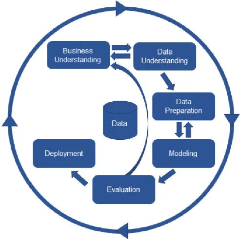
CRISP-DM is the abbreviation of cross-industry process for data mining, which is a standard methodology for planning and implementation of a data mining or machine learning project. It’s robust, flexible, cover all of the aspects, necessary actions required in a typical data mining project. It is also widely used in practice, even with client engagement.

The methodology consists of several steps laid out in a sequential manner. In practice, the steps can be carried out in different order, and even can be iterated multiple times. Each step has a strong connection with other steps, therefore it’s often necessary to jump back and forth among tasks and repeat certain actions. Figure 3-1 shows different phases of CRISP-DM framework model:

(20)

Figure 3-1 CRISP-DM process

3.1 Business understanding

Any project should have a clear objective. Data science project are no exception. Most data science projects are often associated or driven by concrete underlying business objectives. By “business understanding”, this stage emphasizes the understanding of the associating project business objectives, which lays a basis for a proper data mining problem statement in later stage.(Chapman et al., 2000)

3.2 Data understanding

From the business objectives, data mining objectives should be concretely defined and well-stated at this phase. After that, data is collected from relevant sources and then analyzed thoroughly. In this phase, data collection doesn’t necessarily mean the whole process to build a database from start to finish, but mostly querying data from a well-constructed existing database.

(21)

After data collection, initial preliminary checking data also should be carried out in this phase in order to confirm the data is of sufficient quality for later data mining process.

Most importantly, extensive data exploratory analysis process is often carried out in this phase. The goal of exploratory data analysis (EDA) is to create a comprehensive description of the data as well as discover general insights about the data. In other words, EDA helps improving understanding of the data, which is essential for later preprocessing or modeling stage.

3.2.1 Exploratory Data analysis

As its name implies, the goal of exploratory data analysis is to explore some of the main characteristics of the data. The process can employ various techniques from descriptive statistics, hypothesis testing, visualization and so on. EDA can be performed on raw original data, or post-processed data,

Descriptive statistics can be used in this phase to describes each feature (or variable) of the dataset. Hypothesis testing can be employed in order to check if the assumption required for model fitting is meet. Visualization technique (i.e. bar plots, box plot …) can be used to better represent abstract understanding of the data. EDA also encompasses complex mathematical models or algorithms

The explorations obtained from exploratory data analysis often indicate how the data should be prepared or pre-processed in the next stage.

3.3 Data preparation

The goal of this data preparation phase is to transform the raw data into the final dataset that ready to be fed into machine learning models. The reason is that most machine learning models make certain assumptions of the input data. To keep the machine learning model output reasonable and reliable, input data should meet those assumptions of the model. Therefore, data preparation is an indispensable part of any data science or machine learning project. Anomaly detection is also no exception.

In this phase, various preparatory activities can be carried out. The first step is to clean the data, i.e. handling corrupted data, drop unnecessary data and most importantly, handling missing values. Techniques for handling missing values are deletion or imputation. After that, normalization or standardization of the data can also be performed in order to make the data meet certain model assumptions.

(22)

After that, additional pre-processing steps, such as dimension reduction, might also be carried out. Dimension reduction techniques, for example, PCA, aims to represent the original data with a much smaller set of predictors and still maintain the original structure of the data. Such dataset with reduced volume can make training model more efficient and still achieve the same level of performance.

3.4 Modeling

Modelling is often considered as the most important part of any data science project. In this phase, the objective is to select the appropriate model that can achieve the goal defined in the previous phase. There are many machine learning models that can be employed to achieve the same goal. For example, in this anomaly detection setup, one can use any classification method to detect the anomaly. Therefore, different methods should be tested to find out the most optimal method. In this phase, the data scientist should design the training and testing dataset and provide the initial assessment of the model.

3.4.1 Model selection

As discussed in the literature review section, there are many anomaly detection models, divided into 3 groups: unsupervised, supervised and semi-supervised. However, supervised method is highly recommended because of its performance with highly-specific domain application data, its robustness - the ability to detect multiple types of anomaly with one set of predictors. Therefore, the author decided to employ only supervised methods in this thesis, especially because the labeled target data are available from the case company.

3.4.1.1 Scope

Although there are many existing supervised algorithms in literature, in this study, the author decided to limit the scope to only 3 models: random forest, gradient boosting and multilayer-perceptron. Those models are considered as the most popular and favorite choice in practice, as they are robust, fast to train and give well-predictive performance. In contrast to “classic” model like logistic regression, those models do not require any specific assumption about the data, such as independent and identical distributed variables, which is not the case in this thesis.

3.4.2 Random Forest

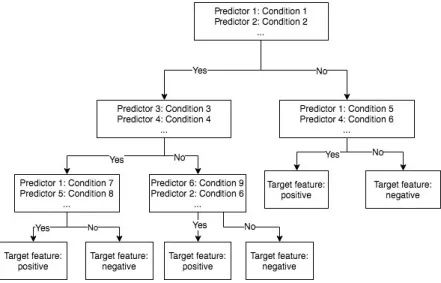
To understand random forest, one needs to know about decision tree model. From the visualization point of view, a decision tree looks like a flow-chart with nodes (i.e. leaf) and

(23)

paths (i.e. branches). In each node, an attribute or feature is tested, and the result is represented by the branch as the path will continue to the corresponding branch. The final node (leaf node) represents the final decision, i.e. the class label. The path from the original node to leaf node represents classification rules. Figure 3-2 represent an example decision tree:

Figure 3-2 Example of Decision tree design

Tree-based methods partition the feature space into a set of rectangles, then fit a simple model (like a constant) in each one. They are conceptually simple yet powerful. One of the advantages of decision tree is that it is low bias model. Theoretically, decision trees are known to be able to capture complex interaction structure in the data. However, they can also be overfitting, as they also learn the noise from the data (Hastie, Tibshirani, & Friedman, 2008). Moreover, as low bias model, decision tree is also high variance model, i.e. a small change in the data can result in a very different tree with different splits. Random forest can fix these issues by employing ensemble techniques with decision tree model. To put it in a simple way, random forest is a mix of different decision tree models.

From the other point of view, decision trees have a number of abilities that make them valuable to be a base learner, namely the ability to handle data of mixed types and the ability to model complex functions.

As Hastie, Tibshirani & Friedman (2008) mentioned in their book, in random forest, decision trees are ensembled by the bagging technique. The major ideas of the technique are:

• Fit the decision tree many times to many sampled versions with replacement of the training set

(24)

The purpose of this bagging technique is to average many noisy but unbiased models in order to reduce the variance. The final model result will have the same bias as (or slightly higher than) the original tree but lower variance.

Random forest employs the same tactics and takes a step further to reduce the variance. Not only taking subset sample of training data, but the model is also trained only on a subset of predictors. This is also called as feature bagging, i.e. random selection of the input variables (feature) in the tree-growing process.

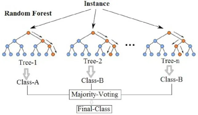
With this design architecture, the bias-variance trade-off still holds true for random forest. Comparing to a single decision tree model, the bias of the forest is usually slightly higher but, due to averaging, its variance also decreases, compensate usually more than for the increase in bias, hence yielding an overall better model. Figure 3-3 sum up the idea of random forest in a simple way:

Figure 3-3 Example Random Forest model architecture

The scikit-learn implementation of random forest is used in the thesis. This implementation combines classifiers using their probabilistic prediction, unlike the original publication in which the final prediction is used. (Breiman, 2001)

In practice, random forest is a popular method, employed in many machine learning problems. Random forest is selected to be used in this case because of its expected higher performance, high accuracy and high robustness.

(25)

3.4.3 Gradient Boosting

Similar to random forest, gradient boosting is also an ensemble method, which combines and averages many weak classifiers (in this case decision tree model) on repeated modified version of the data. However, its difference from random forest is how the data modified after each fitting or so-called boosting iteration: each of the training samples receive a weight 𝑤₁, 𝑤₂, … , 𝑤_𝑁. At first step, these weights are initialized as equal, meaning that the weak learner is simply trained on the original data. After that, those weights are individually modified, and the learning model is refitted to the reweighted data. The weights are individually modified so that those incorrectly predicted training examples at the previous step have their weights increased, meanwhile, the weights are decreased for those that were predicted correctly. As the boosting proceeds, wrong predicted samples in previous weak learner receive more priority in the next learner. In this way, boosting can be a very powerful method, capable of producing highly accurate results. (J. Zhu, 2009)

Gradient boosting employs the same boosting idea, combining with gradient descent algorithm to minimize the loss when adding new models. Mathematically, assuming we have a gradient boosting tree 𝐹(𝑥) with weak learners ℎ_𝑚(𝑥) and weight 𝛾_𝑚 as following:

𝐹(𝑥) = ∑ 𝛾_𝑚ℎ_𝑚(𝑥)

𝑀

𝑚=1

The boosting mechanism is illustrated by the equation

𝐹_𝑚(𝑥) = 𝐹_𝑚−1(𝑥) + 𝛾_𝑚ℎ_𝑚(𝑥)

In which newly added tree ℎ𝑚 tries to minimize the loss 𝐿, given the previous ensemble 𝐹_𝑚−1:

ℎ𝑚 = 𝑎𝑟𝑔𝑚𝑖𝑛ℎ∑ 𝐿(𝑦𝑖, 𝐹𝑚−1(𝑥𝑖) + ℎ(𝑥𝑖))

𝑛

𝑖=1

The minimization problem is solved by steepest descent as follow:

𝐹_𝑚(𝑥) = 𝐹𝑚−1(𝑥) − 𝜃𝑚∑ ∇𝐹𝐿(𝑦𝑖, 𝐹𝑚−1(𝑥𝑖))

𝑛

𝑖=1

In which 𝜃_𝑚 is the step length (often chosen using line search)

3.4.4 MLP Classifier

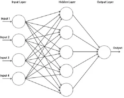
Multi-layer Perceptron (MLP) is a supervised classifier that can learn non-linear function approximators. MLP is a type of artificial neural network, which has an architecture

(26)

made of neuron (nodes) divided into layers. An MLP consists of at least 3 layers, one for input, one for output and a number of hidden layers. MLP is fully-connected, meaning that each node in a layer connects to every node in the next layer. Figure 3-4 illustrates the architecture of a typical MLP:

Figure 3-4 Example of a simple multilayer-perceptron architecture

In each neuron, the output is a weighted-average of the input or output of previous layers) with a nonlinear activation function, as followed:

𝑦𝑘 = 𝜙(∑ 𝑤𝑘𝑗𝑥𝑗)

𝑚

𝑗=0 In which 𝑦𝑘 is the output, 𝑥𝑗 is the input

MLP parameters can be learned using backpropagation techniques. The details of backpropagation:

• First, the parameters are initialized by certain values, then fed to the networks

• Outputs now can be computed in a feedforward manner. Likewise, errors can be computed at the final output and fed backward throughout the network layers

• The gradient is computed using the error obtained from the previous step. One needs to choose the learning rate so that the optimal can be reached

• The parameters are now being updated using the product of the gradient and learning rate

(27)

One of the disadvantages of MLP is that backpropagation doesn’t guarantee to find the global minimum of the function, but only a local minimum. Therefore, the initialization of parameters is very important. (Rumelhart, 1986)

3.5 Evaluation

Even after obtaining the optimal model from the previous stage, it cannot be confirmed that the model would be able to generalize to different datasets. Evaluation phase makes sure that the model is able to perform well in real production and meet the business objectives and needs. Additionally, evaluation tools could also serve as a mechanism to select the optimal model and to discard suboptimal ones.

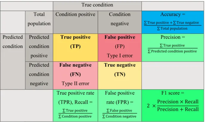
There are many evaluation measures for a machine learning algorithm, such as prediction accuracy, area under ROC curve (AUC-ROC), F1 score etc. Depending on the objective of the project, appropriate evaluation measures will be selected. Table 3-1 shows the confusion matrix and how the evaluation measures are computed from the matrix. Table 3-1 Confusion matrix

True condition Total

population

Condition positive Condition negative

Accuracy = ∑ True positive + ∑ True negative

∑ Total population Predicted condition Predicted condition positive True positive (TP) False positive (FP) Type I error Precision = ∑ True positive ∑ Predicted condition positive

Predicted condition negative False negative (FN) Type II error True negative (TN) True positive rate

(TPR), Recall = ∑ True positive ∑ Condition positive False positive rate (FPR) = ∑ False positive ∑ Condition negative F1 score = 2 ×Precision × Recall Precision + Recall

In this thesis, three evaluation measures will be employed: accuracy, F1 score and AUC-ROC

(28)

3.5.1 Accuracy:

3.5.1.1 Definition

Accuracy is the number of correct predictions divided by the total population. 3.5.1.2 Interpretation

Normally in a typical classification problem which has balance class in target label, if we create a “naive” classifier which predicts all samples to be in one certain class, we would get a baseline classifier with 50% accuracy. The optimal classifier would be expected to have higher accuracy than that.

However, in anomaly detection problem, which has an inherent imbalance class problem, i.e. the ratio would be 90-10 rather than 50-50. If we create a naïve classifier which predicts all samples to be the negative class (the one with the majority), then we would get a baseline model with 90% accuracy, much better accuracy than in the previous case. Therefore, the use of accuracy for anomaly detection might not be appropriate in this case.

3.5.2 F1 score:

F1 score is the harmonic average of precision and recall, in which precision is the number of correctly predicted positive results divided by the number of all predicted positive results, and recall is the number of correctly predicted positive results divided by the number of all positive results.

3.5.2.2 Interpretation

F1 score is the combination of precision and recall, therefore it indicates well the performance of the classifier, especially in the case of imbalance class mentioned above. Let’s assume we create a naïve classifier which classifies all the samples to be negative class, in the case of imbalance data with 90-10 negative-positive ratio. Then TP, FP, TN, FN are 0, 0, 90, 10 respectively. This leads to the F1 score has a value of 0. Thus, F1 score greatly penalizes the naïve classifier for failing to detect any of the positive class, even though the classifier has 90% accuracy. F1 score is selected to be the main measure for selecting and evaluating models in this thesis

(29)

3.5.3 Area under curve - Receiver operating characteristic curve (AUC -ROC):

• ROC curve is created by plotting the true positive rate (TPR) against the false positive rate (FPR) at different discrimination threshold settings. The formulae to compute TPR and FPR is shown in the figure. The purpose of the plot is to demonstrate the performance of a binary classifier at different circumstances.

• Area under curve (AUC): in machine learning, the most common measure from ROC analysis is area under ROC curve (AUC). AUC ROC indicates the capability of the classifier to make a good separation between positive labels and negative labels. 3.5.3.2 Interpretation

Similar to the accuracy measure, AUC ROC would give a score of 0.5 for a naïve classifier, which would predict randomly in the case of balance data. It doesn’t tell us the whole story in the case of imbalance data; however, the score would be lower than the accuracy because it also accounts for different threshold settings

3.6 Deployment

After the model is selected and evaluated to be the optimal one that meets the business needs, it can be deployed into production. The model can be deployed into a local machine or a distributed environment for larger scale dataset. Model deployment is out of scope for this thesis, so it will not be discussed further.

4 Implementation

–

Case study

In this thesis, anomaly detection models are implemented using python, mostly pandas library for data preprocessing and scikit-learn library for modeling.

4.1 Business understanding

As we stated in the literature review, the primary objective of this thesis is to predict failures in advance. By successfully predicting in advance the failure, we can take corrective action and preventive measures, therefore minimize downtime, improve customer experience and reduce operating cost.

With such formulated business objectives and the available dataset, the problem is translated into a supervised problem with multiple target features in this case study.

(30)

4.2 Data understanding

In this case study, each failure is notified by an alarm in the system. The failure or anomalous behavior can occur with different levels of criticality. The data used to predict such alarm failure is collected from a real large-scale LTE network in Finland, as explained in detail in the following subsections.

4.2.1 Data collection

In the LTE network from the case company operator, a large set of performance counters are recorded in each base station on a continuous basis. Each of this performance counter is also referred to as PM in this thesis. From the telecom expert point of view, these are the most relevant data source for predicting the occurrence of alarm failure.

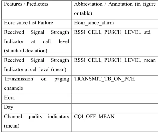
The network consists of over 14000 base stations. The PMs data is collected from a timeframe period of 490 hours or roughly 20 days. Because each station records over ten thousand of PMs as time series, it is impractical to construct and train model on such huge amount volume of data. From earlier work a set of PMs is chosen as predictors for the purpose of alarm prediction as table 4-1 below:

Table 4-1 List of predictors

Features / Predictors Abbreviation / Annotation (in figure or table)

Hour since last Failure Hour_since_alarm Received Signal Strength

Indicator at cell level (standard deviation)

RSSI_CELL_PUSCH_LEVEL_std

Received Signal Strength Indicator at cell level (mean)

RSSI_CELL_PUSCH_LEVEL_mean Transmission on paging channels TRANSMIT_TB_ON_PCH Hour Day

Channel quality indicators (mean)

(31)

Channel quality indicators (min) CQI_OFF_MIN Performance indicator of optimization to avoid handover failure MRO_LATE_HO_NB Transmission on broadcast channel TRANSMIT_ON_BCH

• Channel quality indicator (mean & min): As its name implies, channel quality indicator (CQI) indicates the quality of the communications channel. High CQI indicates that the network is capable of transmit data with large block size, while a low CQI requires the network to reduce the block size. In the case of low CQI, any attempts to transmit the data in large block size will likely results in decoding failures and the needs to retransmit the data again. From the telecom expert point of view, one of the reasons for poor CQI results is hardware failure. Therefore, CQI could provide important predictor for predicting the alarm failure. In the case company data, CQI is represented by two predictors mean and minimum of the quality indicators of all channels from the user equipments (UEs) to the corresponding base stations.

• Performance indicator of optimization to avoid handover failure: Handover is a mechanism in LTE network, enable the mobile user remains connected to the network even he/she moves from one cell to another. A handover process begins when the user moves out significantly of range from the current cell and ends when the user is completely inside the area of new cell. Too early handover can cause ping-pong situation, in which the connection goes back and forth between two base station without becoming stable. Too late handover likely leads to radio link failures. (Bae;Ryu;& Park, 2011) Therefore, the optimization of handover parameter settings to avoid handover failure is important to network performance. As such, the performance indicator of this optimization is chosen for the case study.

• Transmission data on paging and broadcast channel: represent the volume of data transmitted on the corresponding channels. These predictors belong to a broader group of PMs data which represent various throughput values and user activity in the

(32)

network in the up- and downlink. Anomalous changes in these values might indicate malfunctioning hardware or potential hardware failures.

• Received Signal Strength Indicator (RSSI) at cell level: RSSI indicate the level of received power from a radio signal. In this case, the two chosen predictors are computed by taking the mean and standard deviation of RSSI from all signal to the base station. RSSI belong to a broader group of PMs data representing radio interference in the network. based on the radiologist advice, these RSSI-based predictors could be important indicators of potential failure in network hardware devices.

In addition to the set of predictors, a set of target features, representing the alarm failure or anomalies we want to predict, is also available in the dataset. One of the purposes of the thesis is also to determine which type of failures is easier to predict than the other. In this case, the alarms are said to be independent of each other. In another word, at any specific hour, there could be multiple alarms in a specific base station. The list of target feature in this thesis is following:

• Antenna Line Device failure • Cell blocked

• Failure in optical interface • Temperature alarm

• Transmission path failure

• VSWR major alarm (alarm due to VSWR) • VSWR minor alarm

In which VSWR stands for standing wave ratio, indicate impedance mismatch alon g the antenna or transmission line.

As mentioned in the literature review, one characteristic that differentiates anomaly detection with the normal supervised problem is the imbalance ratio of normal and abnormal class. This also holds true in this case. Out of over 6 million data instances in the dataset, the maximum number of any anomalies or alarm is 1500, making the ratio less than 1 to 1000. Figure 4-9 below shows the frequency of each alarm failure occurrence. This poses a difficulty for any typical supervised classifier. Without any special pre-processing or algorithm adjustment, the classifier might not detect any anomaly at all.

4.2.2 Exploratory data analysis

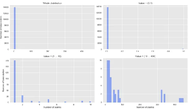
Figure 4-1 shows the distribution of number of alarms for each base station. There are over 14000 base stations. It can be seen that the majority of base stations had experienced zero failures during the recorded time. The bottom two plot gives us a closer look of the

(33)

distribution by only plotting limited support. The bottom left plot tells us that there are over 175 stations with only 1 failure during the recorded hours, and less than 20 stations for each category of base station with 2 to 10 alarms failures. The bottom right plot shows us the base stations with more than 10 alarms during the timeframe. It can be seen that most of the cells had less than 100 alarms during the 490 hours period. On the other hand, there are about 30 or 40 outliers with more than 400 alarms during the period, which means that they experienced the failure most of the time. Telecom expert often refers to those cells as “chronological faulty cells”

Figure 4-1 Distribution of number of alarms per base station

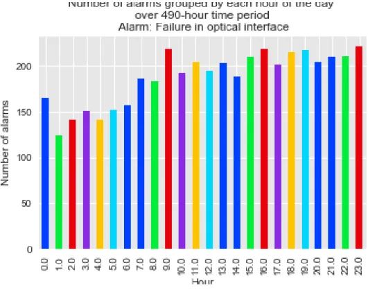
Figure 4-2 showing total number of alarms across all of the cells in each hour of the day. The point of this plot to see whether or not the failures tend to happen at some specific hours during the day. From the plot, we can see that the whole cellular network experienced fewer failures at night (total less than 150 alarms in an hour), although the pattern in each individual base station might be different.

(34)

Figure 4-2 Number of alarms occur at each hour of the day

Similarly, Figure 4-3 shows the number of alarms the whole networks had, hour by hours during the 490-hour timeframe. It can be seen that most of the time the total number of alarms across the network is less than 20. There are some outlier hours at which more than 30 failures happen at once across all over the stations. Predict in advance 4 hour

(35)

Figure 4-4 Distribution of number of timestamps in each base station

Figure 4-4 shows the number of recorded timestamps we have in the dataset. In total there are over 14000 base stations with PM data recorded in 490 hours timeframe. However, there are only over 10000 of them with full 490 timestamps. The remaining have missing timestamps. This poses difficulty in handling missing values and data preparation.

4.2.3 One specific base station

We have 9 PM time series in all over 14000 base station. It is difficult to see all of them at once. Figure 4-5 shows the plot of these time series in a specific base station with Id 10508866

(36)

Figure 4-5 Scaled KPIs and Alarm data from a specific base station

From the plot, it can be seen that alarm tend to happen in cluster, in case one occurs, another one happens shortly. The PM time series seems to follow random patterns; however, different base stations have different patterns for those PMs data.

Figure 4-6 below show the correlation relationship amongst the variable. We have two color spectrums: dark and bright. Dark color represents positive correlation, meanwhile bright color indicates negative correlation. From the plot, it can be drawn that most variables don’t have strong correlation relationship with each other, except the RSSI mean and standard deviation

(37)

Figure 4-6 Correlation matrix of scaled KPIs in a specific base station

4.3 Data preprocessing

4.3.1 Initial processing data

The original data have several issues require fixing, including missing values and discontinuous timestamps. Initial exploratory indicates that missing values are concentrated in certain variables. After removing those variables, there is no null value in the dataset. Because we construct the model in a way that each timestamp is an independent data instance, discontinuous timestamps do not create a big problem for the model. However, discontinuous timestamps also make it unreasonable to use any time series analysis

(38)

technique. For example, extracting seasonality pattern doesn’t provide any good use for later modeling.

After the data is cleaned, the author scaled the data using min-max scaler so that all predictors are within the range [0,1]. It is necessary to scale the data as such because long -range predictors will likely cause bias and heavily skew the anomaly detection model in later phase.

Base on telecom expert advice and earlier studies, the author create a synthetic variable – hour since last alarm, based on each of the target features. The variable is categorical variable, indicating the length of time from the timestamp when last alarm occurs to the current timestamps. It is hypothesized that the failure alarms follow certain patterns, and this synthetic variable could play an important part in predicting the failure.

4.3.2 Oversampling

As mentioned above, class imbalance is a major problem require to be addressed before applying any machine learning or supervised anomaly detection model. In this case study, the author tried different methods to address the issue. One of them is SMOTE sampling, or Synthetic Minority Over-sampling Technique. Using k-nearest neighbor combined with a random factor, the method creates new data points with similar characteristics to the current one. By that mechanism, abnormal data instances are populated to have the same volume as normal data, hence we will have a balanced dataset.

The other method is adjusting the weights of each data instance, so that the weighted average of normal data and abnormal data are equal to each other. Both of the methods are compared and benchmark with the “baseline” method, in which no specific technique is carried out to handling the issue of imbalance class

Figure 4-7 shows the benchmark result for different oversampling technique. Each individual plot represents different model, and within the plots, each group of bar represents the result of different oversampling technique. The blue bar indicates the accuracy of the model, the green bar indicates the F1_Score of the model. As explained later in the evaluation section, the F1_score is the true indicator of how well a supervised model will perform in this case.

(39)

Results

Figure 4-7 Effect of different pre-processing techniques to address imbalance data on the evaluation benchmark

It can be seen that different oversampling techniques bring little to no improvement over classic models such as Naïve Gaussian Bayes and Logistic regression. However, the results are remarkably different with random forest model. By adjusting data instance weight, the f1_score increases by a huge amount, from 0.55 to 0.73. SMOTE sampling doesn’t seem to work that well with random forest, bring the F1_Score to only 0.63.

Based on the result, the author decided to address the imbalance problem by adjusting the data instance weights.

4.3.3 Dimension reduction

The author is also interested in whether or not dimension reduction could bring any extra improvement to the classifier performance, or at least maintain the same performance as with the original dataset. Different dimension reduction methods are also experimented, namely Principle component analysis (PCA) and Factor analysis.

4.3.3.1 Results

Figure 4-8 shows the results of different dimension reduction techniques that were experimented. The first group of bar chart represents the normal modelling without using any dimension reduction technique. The third group of bar chart represents dimension reduction technique which aims to select the best features based on the chi-square statistical. The fourth group of bar chart represents dimension reduction technique which selects the best feature using feature importance scores from other model, in this case another random

(40)

forest. The fifth group of bar chart represents the principal component analysis, or PCA, which attempts to represent the data based on the components that explained the highest variance of the data. Lastly, the sixth group of bar chart represents factor analysis, which has the purpose similar to that of PCA. However, in factor analysis, the components are not necessarily orthogonal to each other, which are in the case of PCA.

Figure 4-8 Effect of different dimension reduction techniques on the evaluation benchmark

From the plot, by comparing all other groups of bar to the first one, it can be seen that using dimension reduction actually doesn’t bring any improvement to modelling. Therefore, it is recommended that the modelling should be carried out with as many features as possible.

4.4 Model selection

In this section, models’ performances are compared to each other to find out which one is the best in this case study. The model selection is carried out by time series cross-validation. Normal cross validation poses a problem to this case, as it would use data from the later period to predict data from earlier period. Time series cross-validation, as illustrated in the following figure 4-9, will eliminate those problems.

4.4.1 Baseline model

In order to verify that a model would give any improvement, a baseline model should be chosen. In this case, the author decided to use a naïve model as the baseline model. Consider a naïve model which assumes every data instance is normal, or non-anomaly, the model

(41)

would have a 100% accuracy, but zero f1 score. Any model that have f1 score greater than zero is considered useful in this case.

4.4.2 Time series cross-validation

Cross-validation has been a common practice for model selection in any science project. However, the technique poses a problem in this case, especially when the author tried to apply machine learning model into time series data. Normal cross-validation folds are selected in such an arbitrarily way that it can use data from the later period to predict the data from earlier period. As such, the author decides to use a special technique of cross-validation for time series data, as referred in literature by (Tashman, 2000) as forward-chaining or (Benítez, 2012) as rolling-origin evaluation. The technique divides the data into multiple folds, using multiple train/test splits, as illustrated in figure 4-9. The main point is that the test set, which will be used to evaluate the model, is always on later period compared to the train set. After evaluating on multiple test set, the result score will be averaged across different folds

Figure 4-9 Number of failure alarms across different time-series cross validation folds

From the plot, we can see that the dataset is divided into training and testing set so that testing sets always come after training set along with the time flow. For each cross-validation fold, the training set is subsequently larger than the previous one. The first two folds, or