Dynamic Modeling of Thermal Management System with Exergy Based Optimization

(1)

Wright State University Wright State University

CORE Scholar

Browse all Theses and Dissertations Theses and Dissertations 2017

Dynamic Modeling of Thermal Management System with Exergy

Based Optimization

Marcus J. Bracey

Wright State University

Follow this and additional works at: https://corescholar.libraries.wright.edu/etd_all Part of the Mechanical Engineering Commons

Repository Citation Repository Citation

Bracey, Marcus J., "Dynamic Modeling of Thermal Management System with Exergy Based Optimization" (2017). Browse all Theses and Dissertations. 1840.

https://corescholar.libraries.wright.edu/etd_all/1840

This Thesis is brought to you for free and open access by the Theses and Dissertations at CORE Scholar. It has been accepted for inclusion in Browse all Theses and Dissertations by an authorized administrator of CORE Scholar. For more information, please contact library-corescholar@wright.edu.

(2)

Dynamic Modeling of Thermal Management System with

Exergy Based Optimization

A thesis submitted in partial fulfillment of the requirements for the degree of Master of Science in Mechanical Engineering

By:

Marcus J. Bracey

B.S.M.E., Wright State University, 2016

2017

(3)

WRIGHT STATE UNIVERSITY

GRADUATE SCHOOL

May 23, 2017

I HEREBY RECOMMEND THAT THE THESIS PREPARED UNDER MY SUPERVISION BY Marcus J. Bracey ENTITLED Dynamic Modeling of Aircraft Thermal Management System with Exergy Based Optimization BE ACCEPTED IN PARTIAL FULFILLMENT OF THE REQUIREMENTS FOR THE DEGREE OF Master of Science in Mechanical Engineering.

Rory Roberts, Ph.D Thesis Director

Mitch Wolff, Ph.D Thesis Director

Joseph Slater, Ph.D, P.E.

Chair, Department of Mechanical and Materials Engineering Rory Roberts, Ph.D

James Menart, Ph.D

Mitch Wolff, Ph.D

Committee on Final Examination

Robert E.W. Fyffe, Ph.D

Vice President for Research and Dean of the Graduate School

(4)

iii

ABSTRACT

Bracey, Marcus J., M.S.M.E. Department of Mechanical and Materials Engineering, Wright State University, 2016. Dynamic Modeling of Aircraft Thermal Management System with Exergy Based Optimization.

System optimization and design of aircraft is required to achieve many of the long term objectives for future aircraft platforms. To address the necessity for system optimization a vehicle-level aircraft model has been developed in a multidisciplinary modeling and simulation environment. Individual subsystem models developed exclusively in MATLAB-SimulinkTM, representing the vehicle dynamics, the propulsion, electrical power, and thermal systems, and their associated controllers, are combined to investigate the energy and thermal management issues of tactical air vehicle platforms. A thermal vehicle level tip-to-tail model allows conceptual design trade studies of various

subsystems and can quantify performance gains across the aircraft. Often one of the main objectives is system efficiency for reduction in fuel use for a given mission. System efficiency can be quantified by either a 1st or 2nd law thermodynamic analysis. A 2nd law exergy analysis can provide a more robust means of accounting for all of the energy flows within and in between subsystems. These energy flows may be thermal, chemical, electrical, pneumatic, etc. Energy efficiency gains in the transient domain of the aircraft's operation provide untapped opportunities for innovation. To utilize a 2nd law analysis to quantify system efficiencies, an exergy analysis approach is taken. This work

demonstrates the implementation of a transient exergy analysis for a thermal management subsystem component found on traditional aircraft platforms. The focus of this work is on the development of a dynamic air cycle machine (ACM) model and implementation of an

(5)

iv

exergy based optimization analysis. This model is utilized in tandem with a bench top ACM experimental unit at the Air Force Research Laboratory’s Modeling, Simulation, Analysis and Testing (MSAT) lab. Individual elements, including compressor, turbines, heat exchangers and control valves have been combined to investigate the behavior of a typical ACM. The experimental test stand is designed and constructed to be used as a method to validate models developed. Combining the results gained from the simulation studies, specifically the exergy analysis, and the experimental setup, a methodology is formulated for system level optimization. By leveraging this approach, future simulation studies can be implemented on various system architectures to generate accurate models and predictive analysis.

(6)

v

ACKNOWLEDGEMENTS

This work was completed under the guidance and direction of Drs. Rory Roberts and Mitch Wolff at Wright State University. I am grateful for the time they dedicated to this project, flexibility in working with my schedule, and most of all, the academic assistance they have provided as my research directors. In addition to their support, this work was supported by students and professionals to include Mark Bodie of AFRL, Dr. Jon Zumberge of AFRL, Sean Nuzum of Wright State, Adam Donovan of Wright State and the support from personnel located at the MSAT laboratory within Aerospace Systems Directorate at AFRL.

I also would like to thank my parents for the support they have provided throughout my academic career and providing me with the foundation for my academic success. Last but not least, I thank my wife, Michelle Bracey, for her understanding and unbounded

support in all my academic pursuits.

Partial support for this project was supplied by the Dayton Area Graduate Studies Institute. The U.S. Government is authorized to reproduce and distribute reprints for Governmental purposes notwithstanding any copyright notation thereon. The views and conclusions contained herein are those of the authors and should not be interpreted as necessarily representing the official policies or endorsements, either expressed or implied, of Air Force Research Laboratory or the U.S. Government.

(7)

vi

TABLE OF FIGURES

Figure 1. (Left) T-S diagram for closed cycle. (Right) Process flow diagram for closed

cycle. ... 6

Figure 2. (Left) T-S diagram for open cycle. (Right) Process flow diagram for open cycle. ... 7

Figure 3. Process flow of the ACM cycle used for the model development. ... 9

Figure 4. T-S diagram for final ACM process ... 10

Figure 5. Tiered approach to modeling and simulation of large scale systems ... 13

Figure 6. ACM test stand process and instrumentation diagram (P&ID) ... 22

Figure 7. ACM Simulink model with boundary conditions. ... 38

Figure 8. State point temperature for the ACM. ... 40

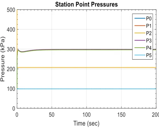
Figure 9. State point pressures for the ACM. ... 41

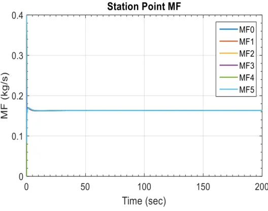
Figure 10. State point mass flows for the ACM. ... 42

Figure 11. ACM shaft speed for turbomachinery. ... 43

Figure 12. Transient exergy destruction rate for ACM components. ... 44

Figure 13. ACM transient exergy destruction rate... 45

Figure 14. ACM component exergy destruction rate with sudden increase in inlet air temp... 46

Figure 15. ACM response when underdamped... 48

Figure 16. Transient exergy destruction rate for underdamped ACM controls. ... 49

Figure 17. ACM response when overdamped... 50

Figure 18. Transient exergy destruction rate for overdamped ACM controls. ... 51

Figure 19. ACM cooling response to increased cooling demand. ... 57

Figure 20. ACM cooling response for varied boundary conditions. ... 58

Figure 21. Boundary conditions for ACM during simulation... 62

(10)

ix

LIST OF TABLES

Table 1. ACM model parameters ... 39

Table 2. Exergy destroyed during simulation with cooling demand step change ... 54

Table 3. ACM mission simulation parameters ... 56

(11)

x

NOMENCLATURE (TEXT)

ACM = Air Cycle Machine

AFRL = Air Force Research Laboratories EDM = Exergy Destruction Minimization EOA = Energy Optimized Aircraft TMS = Thermal Management System MEA = More Electric Aircraft

MIMO = Multiple Input/Multiple Output M&S = Modeling and Simulation ORC = Organic Rankine Cycle VCC = Vapor Compression Cycle WSU = Wright State University

NOMENCLATURE (EQUATIONS)

A = Valve Area

Cp = Specific Heat at Constant Pressure

Cvf = Specific Heat at Constant Volume of Fluid

Cvw = Specific Heat at Constant Volume of Volume Wall

D = Duct Diameter e = Surface Roughness Ecv = Control Volume Energy

(12)

xi

f = Friction Factor

g = Gravitational Constant

h = Specific Enthalpy k = Ratio of Specific Heats

Lduct = Duct Length

M̅_avg = Average Molar Mass

m = Mass mv = Nodal Mass

mwall = Mass of Volume Wall

ṁ = Mass Flow Rate

P = Pressure

P_crit = Critical Pressure

P_ratio = Pressure Ratio

Qc = Cooling Work

Q_heater = Energy Added by Heater

Q̇ = Heat Transfer Rate

R = Ideal Gas Constant

R_u = Universal Gas Constant

t = Time

T = Temperature S = Entropy

U = Internal Energy v = Fluid Velocity

(13)

xii

V = Volume Wnet = Net Work

Ẇ_cv = Rate of Work on Control volume

Ẋ_dest = Rate of Exergy Destruction z = Potential Height

η = Efficiency

ρ = Density

μ = Fluid Viscosity

(14)

1

1. INTRODUCTION

1.1.Problem Overview

Modern day aircraft are transforming as new technology and capabilities are integrated. As new capabilities are integrated, the behavior and overall requirements of the

subsystems are altered. One such system that is transforming and becoming limited is the thermal management system (TMS) [1]. The 5th generation aircraft are the first to operate with thermal deficits [2]. The 5th generation aircraft have reduced ram air heat

exchangers, fueldraulic actuators for thrust and nozzle area control and increased avionics and advanced electronics loads, which all increase the thermal loads on the aircraft.

The next generation aircraft is anticipated to have even higher low quality heat loads which would require a substantial amount of energy to remove the heat. The thermal and power loads are forecasted to increase by an order of magnitude for future aircraft platforms [3, 4]. The TMS must be capable of managing low temperature thermal loads on the aircraft. This is especially true as the advancement of aircraft move toward More Electric Aircraft (MEA). It is then crucial for the TMS design such that the heat load is managed efficiently to produce an Energy Optimized Aircraft (EOA). The TMS impacts the aircraft performance and interacts with the engine, fuel system and the electrical system. In order to properly assess the thermal demands aboard aircraft, research efforts exist to capture the dynamic behavior of these systems through the use of modeling and simulation (M&S). Through these models, the aircraft’s capacity to complete a set of missions without sacrificing performance is better understood. While the models provide tactical insight into the behavior of the aircraft systems, the accuracy of the models must

(15)

2

be quantified. Validation testing must be performed to fully evaluate the aircraft systems and utilize the models. These modeling and validation efforts have evolved from the need to assess the power and thermal demands of current and future aircraft. To account for the energy conversions and losses, exergy analysis is incorporated to account for inefficiencies.

To understand the impact of increasing thermal management requirements, a full vehicle level analysis is needed. Vehicle-level analysis of subsystem interactions could result in significant performance gains across the aircraft, potentially improving the overall effectiveness of future platforms. The development of a vehicle level tip-to-tail (T2T) modeling and simulation tool would allow performance gains to be quantified in a cost effective manner. There are many types of energy being converted onboard the aircraft, chemical, pneumatic, mechanical, electrical and thermal. Therefore, consideration of the interaction between the various systems aboard the aircraft must be assessed. The interface between the thermal, power and electrical management systems is critical to capturing the dynamic behavior of the aircraft system as a whole. Utilizing the

knowledge gained from the studies can provide the necessary information to optimize the performance of the aircraft throughout a mission. Recent work completed by Wright State University (WSU) and the Air Force Research Laboratory (AFRL) focused on the development of a non-proprietary, thermal T2T aircraft model in MATLAB-SimulinkTM [5,6]. In addition, the non-proprietary nature of the model allows the tool to be distributed to various conceptual design groups and researchers. Specifically, it is foreseen that conceptual designers will use the model to conduct design trade studies, allowing the

(16)

3

analysis of multiple design configurations and the resulting subsystem interactions in short time periods [7-9].

1.2.Approach

AFRL has begun work to study different subsystems within aircraft thermal management system architectures, in an effort to accurately predict behavior using physics based models. One component that is incorporated in a typical TMS is an air cycle machine (ACM) [10,11]. The ACM mimics a traditional reverse Brayton cycle where air is ultimately cooled through use of turbomachinery. Air is compressed and then routed through a heat exchanger or series of heat exchangers before being expanded again by a turbine, which provides the mechanical work for the compressor. The current work involves the implementation of a physical test stand of an ACM that will be used to validate a Simulink model. In tandem with the development of a simulation model and bench top test stand, an exergy based analysis is used for system optimization and integration of the ACM into larger, more complex system models.

The modeling approach presented combines both energy and exergy principles based on the 1st and 2nd law of thermodynamics. Combining both these laws provides critical information that can be used for the design, operation, and improvement of systems across multiple platforms. In contrast, only utilizing the traditional 1st law analysis can leave out important information about the system operation that can lead to an inefficient design [12, 13]. The exergy based approach used for the ACM is readily extensible to a systems-level assessment of a more complex TMS architecture model. By this, various subsystems are easily incorporated and integrated into large scale simulation models that include multiple energy domains and platforms such as that within a T2T model.

(17)

4

Simultaneously, the insights from the exergy analysis approach provide a basis for system level optimization, rather than component level. This is accomplished by using exergy destruction as a univariate metric for optimization [14]. Exergy destruction is specifically used because of the need to represent component losses in a consistent system level manner for the ACM model and future aircraft system models. The minimization of exergy destruction provides a single, consistent parameter for

optimization across various subsystems within a large scale system level simulation. By developing a dynamic exergy analysis tool for the ACM, the transient behavior of the ACM is captured. The transient operation highlights where efficiency gains are that were previously untapped for optimization of an ACM. This is especially useful for studying conditions for a system to dynamically update control parameters for maximum

achievable efficiency.

1.3.Thesis Organization

The thesis is organized as follows. Section 2 provides detailed background information pertaining to the ACM thermodynamic cycle and how it is implemented. Following this, the basis for an exergy based analysis is presented for the ACM system. Section 3 details the methodology used to develop the ACM model and bench top test stand. Although the bench top test stand is not studied in depth within this work, it is important to highlight the experimental side of this work as it provides information to the broad scope of the ACM project and how the ACM model was developed. Further, the derivation for the ACM model and exergy analysis is presented. An emphasis is placed on how to use exergy for optimization of the ACM operation. The method used to leverage the exergy analysis for optimal control of the ACM is presented. Section 4 provides the results of the

(18)

5

ACM study. The initial results of the ACM simulation based on the Simulink model are presented. The system optimization of the ACM based on exergy is shown through the dynamic control of the system. Section 5 summarizes the findings of the work performed and outlines key goals reached. Section 6 concludes the work and provides insight for the future work and next steps.

2. BACKGROUND

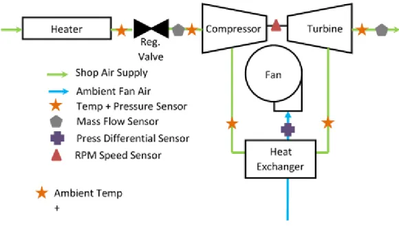
2.1.ACM Architecture

Aircraft thermal management plays a critical role in the performance and effectiveness of an aircraft during flight missions. Due to the high power demand of current aircraft platforms, the thermal loads experienced during operation have increased causing the aircraft TMS to handle higher heat loads than previously designed for. The effect of these high loads correlates to less efficient aircraft or can even cause failure to complete

missions. The TMS aboard aircraft must be designed to handle the specified heat loads experienced throughout the mission. There are two different types of loads, high and low quality heat sources. The high quality sources have high enough temperatures to drive the heat to the heat sinks. The low quality heat sources have low temperature thermal energy that has to be pumped to higher temperatures via refrigeration systems to be dumped to the heat sinks. Electronic thermal loads such as avionics are low quality thermal sources which require refrigeration systems to transfer the thermal energy to the heat sinks. The refrigeration systems are typically reverse Brayton cycles with air as the working fluid, also known as air cycle machines (ACM). The air in a reverse Brayton cycle undergoes the following process in the ideal cycle through each state point. Process 1-2: Reversible,

(19)

6

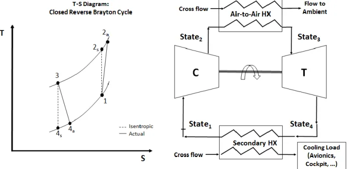
adiabatic compression in a compressor. Process 2-3: Reversible, isobaric heat rejection in a heat exchanger. Process 3-4: Reversible, adiabatic expansion in a turbine. Process 4-1: Reversible, isobaric heat absorption in a heat exchanger. This process is shown in Figure 1 through a process flow diagram and T-S diagram.

Figure 1. (Left) T-S diagram for closed cycle. (Right) Process flow diagram for closed

cycle.

State points for closed Reverse Brayton cycle: 1) Compressor inlet

2s) Isentropic compression outlet 2a) Actual compression outlet 3) HX outlet

4s) Isentropic expansion outlet 4a) Actual expansion outlet

(20)

7

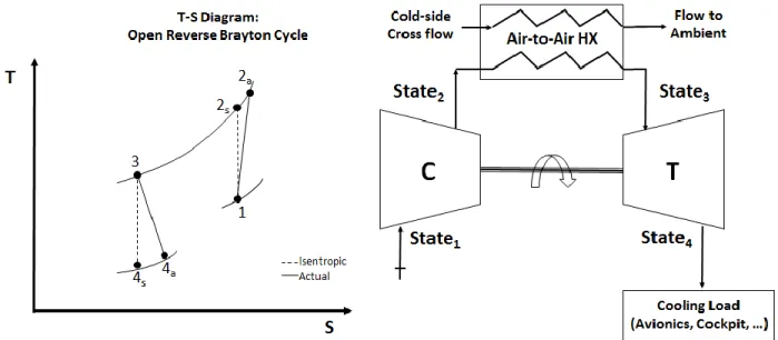
With the actual cycle, there are a few key differences that must be accounted for. The first being that the compression and expansion process is not isentropic, hence there is an exergy destruction rate associated with this process. Second, the pressure drop in the heat exchanger must be calculated to capture the losses other than the inherent losses in the heat exchanger effectiveness. This is the closed loop cycle form of the reverse Brayton cycle. For the model development, the open cycle is used where the inlet air is delivered through a reservoir and the exit air after the cooling turbine dumps into atmosphere. Having the open cycle eliminates the heat exchanger between state point 4 and 1. The open cycle process flow diagram is shown in Figure 2 as well as the state points on a T-S diagram.

Figure 2. (Left) T-S diagram for open cycle. (Right) Process flow diagram for open cycle.

State points for open Reverse Brayton cycle: 1) Compressor inlet from reservoir

(21)

8 2a) Actual compression outlet

3) HX outlet

4s) Isentropic expansion outlet 4a) Actual expansion outlet to load

The open cycle provides various benefits to the closed cycle such as size and weight savings. This process was derived to closely mimic a two-wheeled or bootstrap cycle that is commonly found as an ACM unit on aircraft. The bootstrap cycle provides a

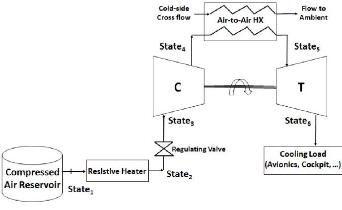
significant increase in cycle efficiency compared to other ACM cycles. In the bootstrap ACM cycle, the compressor is used at the start of the process instead of a fan which is used in a simple ACM cycle. The bootstrap utilizes the power of the turbine to power the compressor. By providing an additional stage of compression at the beginning of the process, a higher efficiency can be achieved. However, the added heat of compression requires an additional heat exchanger between the compressor and turbine [15]. While the process shown in Figure 2 closely mimics the ACM setup used for this work, there are a few key states that are not shown. The final process flow diagram used for this work is shown in Figure 3. As shown, it is an open cycle that utilizes the basic structure of a bootstrap ACM cycle. The inlet air is taken from a shop supply and is modeled as a constant reservoir.

(22)

9

Figure 3. Process flow of the ACM cycle used for the model development.

This process is what was modeled for this work. The experimental setup up also follows this process except for the exit of the turbine at state 6 dumps to ambient. Future

implementation of an experimental cooling load will be incorporated. The cooling load was modeled for the ACM simulation. This cooling load was used as a control constraint for operating the ACM to meet the cooling load demand. The components used in the final process that are not included in the other ACM cycles are the resistive heater and regulating valve. The heater is used to provide a constant heat flux to the air before it enters the compressor. This better simulates the boundary conditions experienced by a typical ACM unit aboard an aircraft. The pressure regulating valve allows for control of the ACM operating speed and cooling capacity. It does this by managing the flow of air from the reservoir and regulates the inlet pressure to the system. The air from the

(23)

10

reservoir is compressed at 100 psi/690 kPa and therefore must be managed to an appropriate pressure before entering the compressor. By appropriately controlling the regulating valve and heat load of the heater, the inlet pressure and temperature of the compressor are controlled and can be used to optimize the ACM performance. Each of these components were modeled and used in the experimental setup of the ACM. The process is further detailed on the S diagram of each state point. Figure 4 presents the T-S diagram for each state point along the ACM cycle used for this work.

Figure 4. T-S diagram for final ACM process

When studying the air refrigeration cycle, it is important to define the operating performance or coefficient of performance (COP). The COP is given by,

(24)

11

𝐶𝑂𝑃 = 𝑄𝑐

𝑊𝑛𝑒𝑡 (1)

where Qc is the cooling capability and Wnet is the total work provided to the ACM. The

COP of an ACM is typically between 0.3 and 0.8 [13,14]. The ACMs are also driven by bleed air from the main engine, which have their own inefficiency associated with the compression of air in the main engine used to mechanically power the ACM. Assuming this conversion of pneumatic energy to work has efficiency of 30% and the COP is 0.4, the overall efficiency of removing low quality heat is 12%. It takes eight times the amount work to move the thermal energy from a cold temperature heat source to a hot heat sink. For example, a 10kW thermal load rate would require more than 80 kW work rate to transfer the heat to a higher temperature heat sink. Due to these inefficiencies, it is important to fully analyze the system performance, specifically the irreversibilities associated with the system. The COP provides a baseline performance parameter for the machine, but it fails to provide a detailed analysis of where the system is experiencing the majority of the lost work potential. For this, a system analysis must be performed which details where the system inefficiencies are most prevalent.

The current work on developing a simulation model of the ACM is complimented with the development of an exergy based analysis on the ACM. An exergy analysis is performed within the ACM model in order to better quantify the overall machine performance. The goal was to perform the exergy analysis of the system to better describe useful energy available to the ACM system. This will define the critical points of efficiencies within the machine as well as direct the power needs of the system as they relate to the overall thermal management system. With an exergy analysis, the design and

(25)

12

operation of components at the system level can be optimizing to reduce the

irreversibilities within the system. Exergy destruction is particularly useful when looking at optimizing the system performance and obtaining a desirable operating point. Using the exergy based approach for system level analysis provides key benefits as opposed to traditional energy based analysis. First, the exergy destruction can be used as a common characterization for irreversibilities across multiple energy domains. This provides a baseline parameter to describe the efficiency of various components used within a larger system [18]. This is useful when analyzing complex systems with multiple components by virtue of a single metric to compare components against. Second, for each component within a system, the exergy destruction rate can be expressed as the sum of each

component’s exergy destruction. This allows for flexibility in the design and change of

system components.

2.2.System Modeling

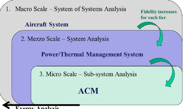
When studying large scale systems such as air or ground vehicles, power plants, or industrial processes, systems engineering can provide useful insight into the behavior of each component and system at large. Capturing the full behavior of the system and ensuring maximum efficiency at the system level poses many obstacles for the engineer to overcome. Griffin examined some common problems faced with systems engineering and capturing system interactions. He proposed a new perspective that focuses on design elegance [19]. This thought process of design elegance has brought forth many new and interesting viewpoints to tackle system level engineering and modeling. One popular answer for creating an elegant system is the utilization of the 2nd law for thermodynamic analysis. The second law provides mathematical formulation to quantify the

(26)

13

irreversibility of a component, process or system. These irreversibilities are captured in an exergy analysis and can be applied to most systems engineering problems. Hence, exergy has been useful in many system level modeling and simulation efforts and has been used for the ACM efforts within AFRL and at WSU. Figure 5 presents a graphic describing the tiered approach to modeling and simulation of large scale systems.

Figure 5. Tiered approach to modeling and simulation of large scale systems

As shown, to study a large scale system such as an aircraft, multiple tiers must be set up each with defined model fidelity. For this study, the ACM, a sub system of an aircraft thermal and power management system, was optimized. The fidelity of the ACM was much higher than a typical aircraft system model as larger scale systems require much more computational power to perform relatively small simulations. Exergy comes into play as a univariate approach to the multi-tier modeling approach. For a large scale

(27)

14

system of systems, exergy can be used as the answer to tying multiple sub systems together to gather an entire picture of the system operation.

Exergy, as a thermodynamic tool, can be used for many different applications such as design, optimization, and assessment of various engineering systems and components. Ahamed and others studied the method of using an exergy based analysis conducted on vapor-compression cycle (VCC) systems to determine the underlining effect of various parameters to improve the overall VCC system efficiency [20]. Similar work was done by Same, S. [21] where an organic Rankine cycle (ORC) was optimized based on the exergy analysis performed for various working fluids. The exergy analysis used in assessing the ORC power cycle was highly beneficial when studying the low quality waste heat of a typical power cycle as a power source for an ORC. Kim et al. [22] further investigated an ORC with an exergy analysis by studying the effect of turbine inlet pressure on the overall exergy destruction of the cycle. It is through an exergy analysis the research team was able to pinpoint the optimal inlet conditions for the turbine inlet. Other various studies have been conducted on the performance of turbo machinery and the use of exergy to detail their performance. Specifically, research on gas turbines in varied load conditions were investigated through exergy to detail the machine performance where an energy analysis would not be sufficient [22, 23]. Exergy has also been used as a

performance criterion for experimental work in the thermodynamics field. Li et al. used an exergy analysis to characterize the performance of an adsorption cold thermal energy storage system [25]. The work detailed where the system inefficiencies were in an effort to predict the best operation on the proposed space cooling system.

(28)

15

In system level studies and analyses, exergy plays a crucial role in defining the system operating parameters and performance. Razmara et al. [26] outlined the method to use exergy-based predictive controls for the HVAC system in an industrial building. By this, operating conditions were chosen for peak performance when needed. Similarly,

performing an exergy analysis can provide knowledge to the theoretical upper limit of the system performance as seen in [27]. Exergy has proven to be useful in many different applications, but it has been shown to be specifically beneficial in system level studies where multiple components are at play. For this work, an exergy analysis similar to the ones mentioned above is utilized to capture the transient behavior of the ACM and highlight the optimal control conditions during operation.

2.2.1. Exergy Analysis Formulation

Utilizing the first law of thermodynamics to perform an energy based analysis for a thermodynamic system can provide useful insight into the behavior of the system. Mathematically, the first law is written as the conservation of energy equation given by,

𝑑𝐸𝑐𝑣 𝑑𝑡 = 𝑄̇𝑐𝑣+ 𝑊̇𝑐𝑣+ 𝑚̇𝑖(ℎ𝑖+ 𝑣_𝑖2 2 + 𝑔𝑧𝑖) − 𝑚̇𝑒(ℎ𝑒+ 𝑣_𝑒2 2 + 𝑔𝑧𝑒) (2)

where cv represents the control volume, i represents inlet state, and e represents the exit state.

However, performing such an analysis is limited. By adding a second law perspective into the analysis, a full description of the thermodynamic system can be achieved. The second law introduces the irreversibility of the system by means of entropy. Another method commonly used to study the irreversibility of a process or system is to study the exergy. Exergy is defined as the maximum reversible work that a system can deliver from

(29)

16

an initial state to the state of the surrounding environment [28]. Mathematically, the flow stream exergy transport,ψ, through a control volume is defined as,

ψ = (ℎ − ℎ₀) − 𝑇(𝑠 − 𝑠₀) +𝑣

2

2 + 𝑔𝑧 (3)

where T0, h0, and s0 are the temperature, specific enthalpy, and specific entropy of the

reference or dead state environment. For a given control volume, thermo-mechanical exergy can be transferred in three different methods: heat transfer, work transfer, or mass transfer. The exergy balance in rate form for a control volume is given by,

𝑑𝑋𝑐𝑣 𝑑𝑡 = (1 − 𝑇₀ 𝑇)𝑄̇𝑐𝑣− (𝑊̇𝑐𝑣− 𝑃0 𝑑𝑉_𝑐𝑣 𝑑𝑡 ) + 𝑚̇𝑖(ψ𝑖) − 𝑚̇𝑒(ψ𝑒) − 𝑋̇𝑑𝑒𝑠𝑡 (4)

where P0 is the reference pressure, 𝑊̇𝑐𝑣 is rate of work across the boundary, and 𝑄̇𝑐𝑣 is the

rate of heat transfer across the boundary. Exergy, unlike energy, is not always conserved. The second law establishes the increase of entropy principle which can be restated using exergy. Exergy must always decreases for an irreversible process. This gives rise to a quantitative measure of the irreversibility of a system, exergy destruction. Exergy destruction is defined as

𝑋̇𝑑𝑒𝑠𝑡 = 𝑇0𝑆̇𝑔𝑒𝑛≥ 0 (5)

Note that for actual processes, the exergy destruction is positive, whereas for a reversible process, the exergy destruction is zero.

Exergy destruction is useful in determining the optimal performance of a system. Exergy analyses based on this formulation have been used extensively to understand system level component interactions and can pinpoint the largest source of irreversibility in the overall

(30)

17

system. Specifically, the minimization of exergy destruction throughout components has been used in many system level optimization problems. Utilizing this analysis, design changes can be made at the component level to improve the system performance [18]. One such example of using an exergy analysis at the design level was to optimized the heat exchanger used in aircraft environmental control systems [29].

2.2.1.1. Exergy Destruction Minimization

Using the thermodynamic optimization approach, exergy destruction minimization (EDM), has proven to be a useful method to system level optimization. One reason for this is that EDM provides a univariate approach across various energy platforms. Because exergy destruction is a common metric, it allows for a direct comparison between

multiple subsystems. For the ACM in study, an operating metric for efficiency commonly used is the COP. This provides useful insight into how the specific ACM subsystem is operating. However, other systems within an aircraft are characterized by additional parameters such as fuel consumption for the aircraft engine. This difference in defining a common parameter is problematic for large system level analyses. Using exergy

destruction as the common metric across multiple domains provides an elegant solution to this problem.

2.2.1.2. Exergy Minimization Control

Exergy destruction provides an objective function for optimal control of systems. Different methods have been used to implement an EDM controller for thermodynamic optimization. One approach that has seen significant research over the past decade is utilizing model predictive control with exergy as a cost function. Model Predictive Control (MPC) predicts and optimizes time-varying processes over a future time horizon.

(31)

18

MPC is useful for MIMO plants where the demands of the plant are well known. For a transient simulation, MPC is used to provide real time control of a system in an effort to optimize the system operation. Jain was able to use exergy destruction as the objective function in the control of an integrated energy system [30]. The work implemented an exergy based MPC approach with the goal to achieve maximum efficiency while meeting the demand of the energy system. Hadian and Salahshoor used exergy losses as the criterion to analyze a MIMO industrial process [31, 32]. By performing an exergy based analysis, information was gained as to where the processes that consumed the majority of exergy were. The process was optimized with MPC by reducing the exergy losses

through improving control performance. While MPC provides many benefits for control systems, the intense computational demands limit the actual utilization in environments where the computing platform is constrained. For this work, a method for optimal control is developed based on exergy destruction that can be readily employed without

introducing additional computational burden. By using a rigorous study of basic PI controllers and gain scheduling, the optimal control of the ACM is studied through simulation for many various different environments.

3. METHODOLOGY

To develop the ACM bench top experimental unit and the corresponding Simulink model, automotive components for the ACM were selected for the turbomachinery and heat exchanger. By employing automotive turbochargers, a bootstrap ACM architecture can be designed which mimics traditional ACM's found on multiple aircrafts. The

(32)

19

implemented in actual aircraft. By validating the component models with the experimental bench top unit, these component models can then be used in the

construction of future system model architectures. The methodology generated through this work can then be exploited for the development of a more accurate modeling approach.

3.1.Air Cycle Machine Description

The transient ACM model developed in the MATLAB-SimulinkTM environment is modeled after the physical bench top test setup of an ACM. The ACM simulation model will be used in tandem with the bench top setup of the ACM. This allows for validation of the model in order to assess the accuracy of the model. The ACM model and bench top test unit both use a series of controllers for various inputs to the system that control the ACM system performance.

Inputs and boundary conditions for the ACM model include: 1) inlet air temperature, pressure, and humidity; 2) fan air temperature, pressure, and mass flow; 3) ambient temperature, pressure, and humidity; 4) regulating valve control pressure; and 5) heater load. The majority of these boundary conditions can be controlled and/or measured through a series of controls/sensors giving the ACM model the flexibility needed for experimental validation. Upon running the model, outputs are the station point temperature, pressures, and mass flows before and after each main component in the ACM.

Within the model, each key component of the ACM is included. The whole ACM system is divided into subsystems that describe the individual components as well as the ducting

(33)

20

before and after each component. The first subsystem is the heater. This heater is used to indirectly control the temperature of the flow entering the compressor. The next

subsystem is the regulating valve, which is connected to the heater by another duct system. The regulating valve is composed of three sections, input and output nodes and the valve itself. This is the critical control device for the system that regulates the inlet pressure to the compressor. The next block is the compressor and turbine combination. Unlike the previous subsystems, this one is controlled by performance maps. These maps were numerically generated with the knowledge of the geometry and design through turbomachinery design software. Between the compressor and turbine is a heat

exchanger. The heat exchanger has four components that are modeled. It has an inlet flow chamber for the hot air coming from the compressor, an outlet flow chamber for the hot air traveling to the turbine, an inlet flow chamber for the cold crossflow, and an outlet flow chamber for the cold crossflow. Both of the inlet and outlet blocks for the hot air function similarly. For the cross flow, a fan with constant flow rate will be used as the cooling medium within the heat exchanger.

3.2.Bench Top Test Unit

When performing M&S studies, it is important to gain an understanding of how

accurately the model predicts the behavior of the system. Due to the limited scope of this work, experimental data for an exergy analysis has yet to be completed. Because the model was developed from the experimental unit, the description of the bench top unit is outlined in the following sections. Future work will look to study how to properly investigate and validate the ACM simulation exergy analysis to experimental results.

(34)

21 3.2.1. Experimental Setup

At its core, a Garrett 1548 turbocharger is used with a Vibrant Performance 12616 intercooler as the heat exchanger. A medium sized fan is used to move ambient air

through the cold side of the heat exchanger. The fan was sized to meet the demands of the system and is estimated to provide up to 60 lbs/min ( 0.45 kg/s) of airflow through the heat exchanger. This flow rate ensures that the heat exchanger effectiveness is high enough that the temperature to the turbine inlet is at a reasonable point.

In general this system architecture has three main controllable inputs to determine the performance. The first is the amount of heat applied to the pressurized air supply before entering the inlet of the compressor. This heat load serves as a disturbance to the system that is controlled to manage the temperature of the air at the compressor inlet. Second, the regulating valve controls the inlet flow pressure to the compressor. The pressure is

limited to between 20 psia / 137 kPa and 45 psi / 310 kPa. These values come from analyzing the compressor efficiency based on the compressor maps. This is an important control variable because it plays a large role in the operating speed of the turbomachinery and overall performance. Last, the fan flow rate across the cold side of the heat exchanger is controlled. The fan flow across the heat exchanger represents the bypass air across a typical ACM heat exchanger. For a typical mission, this airflow varies over the course of a mission. The CFM output of the fan will determine the effectiveness of the heat

exchanger.

3.2.2. Process and Flow Diagram

There are variables that cannot be controlled throughout a test. The air from the in-house air supply has temperature and pressure that vary as the in-house air supply cannot be

(35)

22

controlled. Sensors will measure these parameters on the physical system and will be adjusted in the model to mimic the testing conditions. In addition to these sensors measuring the air supply, a series of other sensors will be used to collect the data during operation. Figure 6 provides a schematic of the system architecture as well as the station points where sensors will be located to collect the desired data.

Figure 6. ACM test stand process and instrumentation diagram (P&ID)

For outputs from the experiment, there are several places where data is taken that can be compared later to the model. This requires a flexible model that is easily adjusted to match the experimental conditions. The experimental design allows for temperature and pressure readings at many points along the air flow. These two parameters are measured before and after each of the major components. Additionally, the mass flow is measured in the hot flow after the regulating valve. The mass flow is also measured from the fan on the cold air flow using a pressure differential sensor. The speed of the turbocharger is

(36)

23

measured at the shaft connecting the two. Through collection of data, the test stand will provide crucial data to validate the ACM model.

3.2.3. ACM Component Selection

The components used in both the model and the experimental bench top test stand were chosen based on various parameters. The physical test stand of the ACM incorporates readily available parts whose information is easily obtained. The decision was made to design and build the ACM from automotive parts including a turbocharger for the turbine and compressor and an intercooler for the heat exchanger. The machine specifications for each of the parts used are easily obtained to fully define the system in the model. The core components of the ACM are the turbine, compressor, and heat exchanger. The model development of the ACM requires detailed performance maps for the turbo-machinery and heat exchanger. The first step in generating the turbo-turbo-machinery maps was to select the appropriate machinery. The sections below describe the turbo-machinery selection process as well as the development of the compressor and turbine performance maps. The heat exchanger was then sized according to the demands of the turbomachinery selected. The heat exchanger selected had to be large enough to provide enough heat transfer between the turbine and compressor such that the turbomachinery would be operating at the highest efficiency. A heat exchanger sizing routine was developed to generate initial performance maps for the ACM heat exchanger. The heat exchanger performance map was generated based on the size, surface treatment, geometry, and material.

(37)

24

ACM’s used in automotive applications closely mimic those used in the aerospace industry. Both have a centrifugal compressor and turbine, but the air stream conditions entering each component, compressor and turbine, are much different in the automotive application when compared to the aerospace ACM application. In the automotive application, the compressor inlet air stream is at ambient pressure and temperature conditions while the turbine accepts hot exhaust gases in the range of 1500oF / 816oC or more. In the bootstrap ACM application, the compressor inlet air stream conditions are at elevated pressures and temperatures, and the turbine inlet conditions are at lower

temperatures, in the range of 120oF / 50oC. These large differences in compressor and turbine inlet conditions, between the automotive and aerospace ACM application, can result in improper compressor and turbine matching.

In order to minimize compressor and turbine matching issues, research was completed to identify the most appropriate turbocharger for the aerospace ACM application from readily available turbochargers in the market. The turbochargers were selected by matching the actual mass flow of the compressor and turbine with inlet boundary

conditions of 25psia/172 kPa and 200oF/94oC for the compressor and 50psia/345 kPa and 120oF/50oC for the turbine. These are the boundary conditions of the compressor and turbine that the ACM bench tests were designed to handle. Through basic turbocharger research, the manufacturer chosen was Garret by Honeywell [33]. The company provided compressor and turbine maps for each turbocharger based on the corrected compressor mass flow. Garret provides over 80 different turbochargers that could be used for this system. In order to narrow the selection to one, the performance maps of the

(38)

25

turbochargers were analyzed. The needed corrected mass flow was determined for the operating boundary conditions and the actual mass flow was determined, by

𝑚̇_𝑎 = 𝑚̇_𝑐 𝑃_𝑎 14.7𝑝𝑠𝑖𝑎 ⁄ √𝑇𝑎⁄_{519 𝑅} (6)

where ma is the actual mass flow (ppm), mc is the corrected mass determined from the

compressor map (ppm), Pa is the inlet compressor pressure (psia), and Ta is the inlet

compressor temperature (R). The actual mass flow is determined from the above equation and compared to that of the turbine. Using the turbine maps at a constant pressure ratio, the corrected turbine mass flow is determined. For a perfectly matched system, the ratio of the turbine and compressor corrected mass flow would be 1. After this analysis, the GT1548 turbocharger provided the best match for the demands of the ACM bench top test stand.

In addition, to the compressor to turbine mass flow matching, the ACM test bench mass flow must be compatible with the available heater and facility air. The 25kW heater used to preheat the house air has the ability to increase the facility air temperature to the 200oF / 94oC required by the compressor. The compressor mass flow requirement is also well below the facility air capability of 180 pounds per minute (ppm) / 1.36 kilograms per second (kg/s) at 100psia / 690 kPa. Because of the compressor and turbine mass flow matching and mass flow capability with the facility air and existing heater, the GT1548 was selected for the ACM test bench turbo-machinery.

(39)

26

To accurately model the ACM system, performance maps were generated for the compressor and cooling turbine. These maps were numerically generated with the knowledge of ACM geometries and design by means of turbomachinery software package. These performance maps are implemented in the ACM model and include calculations based on mass flow, pressure ratio, shaft speed, and efficiency.

ConceptsNREC [34] is a company that offers software packages that calculate the necessary performance characteristics of radial turbines and compressors. The software packages output the performance map characteristics with all geometry and design considerations taken into account. This allows us to export the performance maps from the software and include in the overall model. The maps created were developed on a trial basis of the ConceptsNREC software COMPAL and RITAL.

3.3.ACM Model Development

In this work, all modeling efforts were done in the MATLAB-SimulinkTM environment. The ACM model is developed without iteration loops (algebraic constraints) and all states are continuous. This approach is very important for complex system level simulations of stiff dynamic systems. By modeling all the significant states as continuous states and not steady-state approximations with discontinuities, advanced numerical solvers for stiff systems may be used. Numerical solvers for stiff systems rely on the Jacobian matrix and thus require accurate approximations for gradients of all continuous states. The following sections provide a detailed description of the modeling approach for the transient ACM model.

(40)

27

For the ACM model, a nodal volume approach was taken to model the flow between system components. This approach includes three main elements being modeled; 1) A flow resistive element which represents the ducting, 2) Nodal volumes before and after system components, 3) System components such as regulating valve, turbine,

compressor, etc. The mass continuity and energy balance equations were applied to nodal volumes both before and after major components, generating nodal pressure and

temperature states. Flow resistance equations based on ducted flow were used between nodal states to determine the mass flow between nodes. The nodal volumes inputs are based on the resistive flow calculations from the ducting and boundary conditions. The Swamee and Jain correlation is used to determine the duct mass flow [35].

𝑚̇ = (𝜌(−0.965)√∆𝑃 ∗ 𝐷 5 𝜌𝐿 ) [ 𝑙𝑜𝑔 ( ( 𝑒 3.7𝐷) + √3.17 ∗ (𝜇_𝜌)2𝐿𝜌 ∆𝑃 ∗ 𝐷3 )] (7)

where 𝑚̇ is the fluid mass flow, 𝜌 is the fluid density, ∆𝑃 is the differential in pressure, D is the duct diameter, L is the duct length, 𝑒 is the surface roughness, and 𝜇 is the fluid viscosity. The direction of the mass flow through the resistive ducting elements is

determined by the differential in pressure across the element. The differential in pressure is based on the difference in the nodal volume pressure after the duct and the boundary conditions at the duct inlet. This method requires an initial nodal pressure that represents the initial pressure within the system components. The fluid mass within each nodal volume is determined from the mass continuity shown below,

(41)

28

∫ 𝑑𝑚_𝑉 = ∫(𝑚̇_𝑖− 𝑚̇_𝑜)𝑑𝑡 (8)

where mi is the mass flow entering the nodal volume, mo is the mass flow exiting the

nodal volume, and mV is the nodal mass.

The energy conservation equation is used to determine fluid nodal temperature shown below,

𝑑(𝑚_𝑉𝑢_𝑉)

𝑑𝑡 = 𝑚̇𝑖ℎ𝑖 − 𝑚̇𝑜ℎ𝑜

(9)

where hi is the inlet stream enthalpy, ho is the outlet stream enthalpy, and uv is the nodal

volume internal energy. By incorporating the volume wall thermal capacitance into (9), the energy equation becomes

𝑑(𝑚_𝑉) 𝑑𝑡 𝑢𝑉+ (𝑚𝑉𝐶𝑉𝑓+ 𝑚𝑤𝐶𝑉𝑤) dT dt = 𝑚̇𝑖ℎ𝑖 − 𝑚̇𝑜ℎ𝑜 (10) 𝑑𝑇 𝑑𝑡 = (𝑚̇𝑖ℎ𝑖 − 𝑚̇𝑜ℎ𝑜−𝑑(𝑚𝑉 ) 𝑑𝑡 𝑢𝑉) (𝑚_𝑉𝐶_𝑉𝑓+ 𝑚_𝑤𝐶_𝑉𝑤) (11)

where Cvf is the specific heat at constant volume of the fluid, mwis the wall mass, Cvw is

the specific heat of the wall and T is the temperature of the element. The pressure at the node is found through the use of the ideal gas law shown,

𝜌 = 𝑚 𝑉 ⁄ (12)

(42)

29

where V is the nodal volume, R is the ideal gas constant, T is the nodal temperature, and P is the nodal pressure.

3.3.1. System Components

The ACM model revolves around modeling five core components. These are the heater, regulating valve, turbine, heat exchanger, and compressor. As mentioned, the ducting between each system elements was modeled as a resistive flow element. The basic derivation for each system model is described in the following sections.

Heater

The first subsystem is the heater. This heater is used to indirectly control the temperature of the flow entering the compressor. This acts as a disturbance to the system and will have a large impact on the exergy destruction and overall performance of the ACM. The conservation of mass for this system is shown in the following equation.

𝑚 = ∫ 𝑚̇𝑖𝑛− 𝑚̇𝑜𝑢𝑡𝑑𝑡 (14)

With the mass accumulated in the system, the pressure can be found using ideal gas law in the following equation.

𝑃 =𝑚𝑅𝑇

𝑉 (15)

The temperature after the heater element is found by the energy equation.

𝑑𝑇 𝑑𝑡 = 𝑄_{ℎ𝑒𝑎𝑡𝑒𝑟}+ 𝑚̇ℎ_𝑖𝑛− 𝑚̇ℎ_𝑜𝑢𝑡 −𝑑(𝑚𝑣) 𝑑𝑡 𝑈 𝑚_𝑣𝐶_𝑣𝑓+ 𝑚_{𝑤𝑎𝑙𝑙}𝐶_𝑣𝑤 (16)

(43)

30

The 𝑄ℎ𝑒𝑎𝑡𝑒𝑟 represents the energy that the heater delivers to the airflow. The enthalpy

terms are calculated using relationships with temperature for dry air and then the flow rate.

The heater acts as a heat load on the incoming air into the ACM. This heat load is representative of the heat of compression from the main engine compressor. By controlling the amount of heat input, the ACM can be run through various cycles that simulate different operating conditions and environments for the ACM. Thus, the amount of heat input into the air before entering the ACM is defined as a critical control

parameter for operation of the ACM.

Regulating Valve

The next subsystem is the regulating valve, which is connected to the heater by another duct system. The regulating valve is composed of three sections, input and output nodes and the valve itself. The input and output nodes are identical. They operate in a similar manner to the heater with the following equation set finding the accumulated mass in the system using conservation of mass and ideal gas equation to find the pressure. This element is the main control element for the ACM model. The inlet pressure which is determined by the valve directly affects the operating conditions for the ACM.

The modulating valve is modeled as an ideal gas, one-dimensional, steady, frictionless, and adiabatic flow through a converging nozzle. The valve area is determined by a feedback control system that compares the desired pressure to the pressure on the outlet node. The mass flow is calculated using,

(44)

31 𝑚̇ = 𝐴√( 2𝑘 𝑘 − 1) (𝑃𝑚𝑎𝑥)(𝜌) (𝑃𝑟𝑎𝑡𝑖𝑜 (_𝑘2) − 𝑃_{𝑟𝑎𝑡𝑖𝑜} (𝑘+1) 𝑘 ₎ ₍₁₇₎

The regulating valve is the key component that is used as a control parameter for the ACM. By regulating, the inlet pressure, the operating conditions of the ACM are determined. The pressure after the regulating valve is defined as a critical control parameter for operation of the ACM like the heat input.

Turbine/Compressor

The compressor and turbine model used in this effort determines the outlet pressure, temperature, and power given shaft speed and inlet pressure and temperature. The power generated by the turbine is matched to the power consumed by the compressor. The compressor and turbine models use performance maps which relate pressure ratio, corrected mass flow, corrected speed, and efficiency.

The corrected mass flow associated with the compressor and turbine is calculated by,

𝑚̇_𝑐 = 𝑚 ̇ √𝑇𝑖⁄𝑇_𝑠𝑡𝑑 𝑃𝑖 𝑃𝑠𝑡𝑑 ⁄ (18)

where 𝑚̇_𝑐is the corrected mass flow, 𝑚 ̇is the actual compressor mass flow, Ti is the

compressor inlet temperature, Tstd is standard temperature, 519oR, Pi is the compressor

(45)

32

𝑁_𝑐 = 𝑁

√𝑇𝑖⁄𝑇_𝑠𝑡𝑑𝑃𝑖⁄𝑃_𝑠𝑡𝑑

(19)

where N is the actual speed and Nc is the corrected speed.

The compressor and turbine models use variable specific heat methodology to determine the outlet temperature and power.This is done by calculating the change in entropy to determine isentropic efficiency. The ideal gas entropy change is given by,

𝑠₂− 𝑠₁ = ∫ 𝐶_𝑝 2 1 (𝑇)𝑑𝑇 𝑇 + 𝑅𝑙𝑛 𝑃₂ 𝑃₁ (20)

where T is the flow temperature, R is the ideal gas constant, P2 is the outlet pressure, P1 is

the inlet pressure, s2 is the outlet entropy, s1 is the inlet entropy, and Cp(T) is the specific

heat based as a function of temperature. To find the entropy property at the given temperature, the entropy air property is found using,

𝑠𝑜 = ∫ 𝐶𝑝 𝑇 0 (𝑇)𝑑𝑇 𝑇 (21)

The outlet isentropic entropy is found along with the compressor inlet pressure, inlet temperature, outlet pressure along with the so air property. With the outlet isentropic entropy known, so is used to calculate the isentropic exit temperature.

For the compressor, the actual outlet temperature is determined by first calculating the compressor inlet and isentropic outlet enthalpy along with the compressor efficiency, or

𝐻₂ =(𝐻2𝑠− 𝐻1) 𝑒𝑓𝑓 + 𝐻1

(46)

33

where H2 is the actual compressor outlet enthalpy, H2s is the isentropic compressor

enthalpy, H1 is actual compressor inlet enthalpy, and eff is the compressor efficiency. The

outlet enthalpy is used to determine the actual compressor outlet temperature. Finally, the compressor power is determined by,

𝑃𝑐 = 𝑚̇(𝐻2− 𝐻1) (23)

For the turbine, the actual outlet enthalpy is found by,

𝐻₄ = 𝐻₃− (𝐻₃− 𝐻_4𝑠)𝑒𝑓𝑓 (24)

where H4 is the actual turbine outlet enthalpy, H4s is the isentropic turbine enthalpy, H3 is

actual turbine inlet enthalpy, and eff is the turbine efficiency. The outlet enthalpy is used to determine the actual compressor outlet temperature. The power delivered by the turbine is determined by,

𝑃𝑡= 𝑚̇(𝐻3− 𝐻4) (25)

Based on these equations, the outputs of the turbine and compressor are given. The actual outlet mass flow and outlet temperature are output to a nodal element which determines the outlet pressure and temperature.

Heat Exchanger

The ACM heat exchanger is used to reject heat from the compressor outlet air stream to the environment before entering the turbine. The HX model employs effectiveness and pressure drop maps based on test data and performance prediction methods taken from Kays and London [36]. This method is easily incorporated into the ACM model.

(47)

34

The heat exchanger has four nodal volumes used to model the flow through both the hot and cold side. It has an inlet flow chamber for the hot air coming from the compressor, an outlet flow chamber for the hot air traveling to the turbine, inlet chamber for cold air stream from the fan, and an outlet chamber for cold air exiting the heat exchanger. Both of the inlet and outlet blocks for the hot air function similarly.

The 𝑄_{ℎ𝑒𝑎𝑡 𝑡𝑟𝑎𝑛𝑠𝑓𝑒𝑟} in the heat exchanger is calculated by,

𝑄_{ℎ𝑒𝑎𝑡 𝑡𝑟𝑎𝑛𝑠𝑓𝑒𝑟}= 𝑒𝑓𝑓 (𝑚̇_{ℎ𝑜𝑡 𝑜𝑢𝑡} 𝐶_{𝑝 ℎ𝑜𝑡}(𝑇_{ℎ𝑜𝑡 𝑖𝑛}− 𝑇_{𝑐𝑜𝑙𝑑 𝑖𝑛})) (26)

where 𝐶𝑝 ℎ𝑜𝑡 is the specific heat for the hot air stream and 𝑒𝑓𝑓 is the heat exchanger

effectiveness, which is found using a lookup table based on the surface treatment, geometry, and material of the heat exchanger. The hot fluid properties, including

temperature are determined by the inlet and outlet flow chambers. The fluid temperature is found using the energy equation as shown below.

𝑑𝑇 𝑑𝑡 = 𝑄ℎ𝑒𝑎𝑡 𝑡𝑟𝑎𝑛𝑠𝑓𝑒𝑟+ 𝑚̇ℎ𝑖𝑛− 𝑚̇ℎ𝑜𝑢𝑡−𝑑(𝑚𝑣 ) 𝑑𝑡 𝑈 𝑚_𝑣𝐶_𝑣𝑓+ 𝑚_{𝑤𝑎𝑙𝑙}𝐶_𝑣𝑤 (27)

The cold pressure and the hot fluid mass flows are determined by look up tables based on the geometry and surface finish of the heat exchanger.

3.3.2. Component Exergy Derivation

By employing the 2nd law of thermodynamics, the efficiencies of the ACM and

performance are captured. An exergy analysis provides insight into the available energy of the system and exactly where the inefficiencies of the machine are located. By

(48)

35

analyzing the exergy destruction rate, the quantity of the work capacity that a system loses during a process is quantified. To fully assess the total irreversibility in the ACM, a system level approach was taken. By modeling the individual components within the ACM model, the inefficiencies within the total ACM can be more directly analyzed. The main components studied include the turbine, compressor, and heat exchanger. These are the core system components of the ACM and are the main source of exergy destruction. The development of the exergy destruction model is described in the following sub sections.

Turbine/Compressor

The equations below are used to calculate the rate of exergy destruction for the turbine and compressor sub systems used in the ACM. Mathematically, these two have identical exergy destruction computations. Both are developed on a molar basis for a more robust model. 𝑋̇_{𝑑𝑒𝑠𝑡} = 𝑚̇𝑇0∆𝑠𝑔𝑒𝑛 𝑀̅_𝑎𝑣𝑔 (28) 𝑀̅𝑎𝑣𝑔 = 𝑥𝑎𝑖𝑟∗ 𝑀̅𝑒𝑙𝑒𝑚𝑒𝑛𝑡 (29) ∆𝑠𝑔𝑒𝑛= 𝑐𝑃∗ 𝑙𝑛 𝑇_𝑜𝑢𝑡 𝑇𝑖𝑛 − 𝑅𝑢∗ 𝑙𝑛 𝑃_𝑜𝑢𝑡 𝑃𝑖𝑛 ₍₃₀₎

The turbine and compressor exergy equations used in this work were developed and implemented in the model. Through this analysis, the total exergy destruction through the turbomachinery of the ACM was quantified.

(49)

36 Heat Exchanger

The heat exchanger exergy balance equations used in this work were developed and implemented in the model. The model splits the heat exchanger into three different flow streams to compute the transient entropy generated: 1) the cold side flow, 2) the hot side flow, and 3) the heat exchanger mass. The equations below are used to calculate the exergy balance of the heat exchanger, where c is for cold air, h is for hot air and HX is for heat exchanger. These assume constant mass in the control volume and constant pressure.

𝑚𝑐 𝑐𝑝,𝑐 𝑇_𝑐 𝑑𝑇 𝑑𝑡 = −𝑄̇_𝑐 𝑇_𝐻𝑋 + 𝑚̇(𝑠𝑖𝑛,𝑐− 𝑠𝑜𝑢𝑡,𝑐) + 𝑆̇𝑔𝑒𝑛,𝑐 (31) 𝑚ℎ 𝑐𝑝,ℎ 𝑇_ℎ 𝑑𝑇 𝑑𝑡 = −𝑄̇_ℎ 𝑇_𝐻𝑋 + 𝑚̇(𝑠𝑖𝑛,ℎ− 𝑠𝑜𝑢𝑡,ℎ) + 𝑆̇𝑔𝑒𝑛,ℎ (32) 𝑚𝐻𝑋 𝑐_{𝑝,𝐻𝑋} 𝑇𝐻𝑋 𝑑𝑇 𝑑𝑡 = 𝑄̇_𝑐 + 𝑄̇_ℎ 𝑇𝐻𝑋 + 𝑆̇𝑔𝑒𝑛,𝐻𝑋 (33)

By utilizing the additive property of exergy, the overall exergy destruction rate for the heat exchanger is found by,

𝑋̇𝑑𝑒𝑠𝑡= −𝑇0(𝑆̇𝑔𝑒𝑛,𝑐𝑜𝑙𝑑+ 𝑆̇𝑔𝑒𝑛,ℎ𝑜𝑡+ 𝑆̇𝑔𝑒𝑛,𝐻𝑋) (34) 𝑋̇_{𝑑𝑒𝑠𝑡} = −𝑇₀ ( 𝑚_𝑐𝑐𝑝,𝑐 𝑇_𝑐 𝑑𝑇 𝑑𝑡− 𝑚̇(𝑠𝑖𝑛,𝑐− 𝑠𝑜𝑢𝑡,𝑐) + 𝑚_ℎ𝑐𝑝,ℎ 𝑇_ℎ 𝑑𝑇 𝑑𝑡− 𝑚̇(𝑠𝑖𝑛,ℎ− 𝑠𝑜𝑢𝑡,ℎ) + 𝑚_𝐻𝑋𝑐𝑝,𝐻𝑋 𝑇_𝐻𝑋 𝑑𝑇 𝑑𝑡 ) (35)

(50)

37

This provides a fully transient model of the heat exchanger utilized within the ACM. With the above development of the exergy destruction rate model for the heat exchanger, the overall exergy destruction rate for the ACM during operation was assessed. Both transient and steady state values were studied in order to fully understand the behavior of the ACM.

4. RESULTS

The results shown are that as simulated by the ACM Simulink model. It is important to note that the results are not that of the experimental bench top test stand of the ACM. Although this work compliments that of the experimental work, the simulation results are separate. The model was developed based on the bench top test stand of an ACM

developed and is used for accurate, predictive measures of the experimental ACM.

4.1.Preliminary ACM Analysis

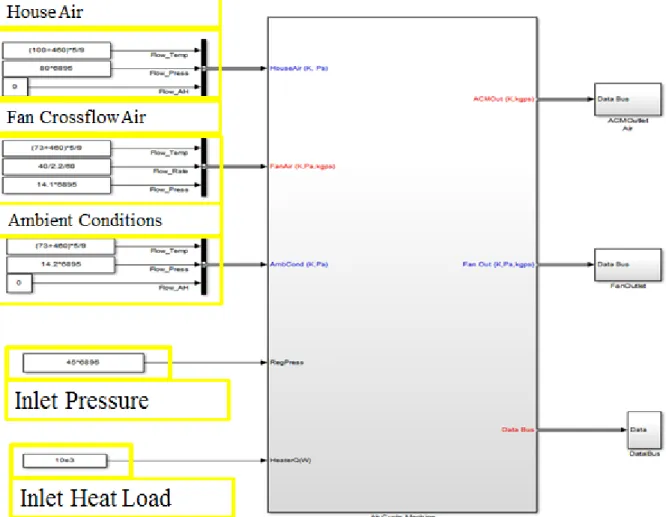
The ACM model after full development is shown in Figure 7. As seen, the main inputs included are the house (compressed) air, fan cross flow, ambient air conditions, inlet pressure, and inlet heater load. By varying each of these boundary conditions, the ACM can be simulated in a number for different ways. Each input can be changed to emulate the different environments the ACM will operate in. The main controlling variable for the ACM is the inlet pressure as this is directly controlled by a regulating valve and will determine the performance of the ACM. The other inputs can be viewed as disturbances or environmental variables in that they vary with different simulations, but these cannot be directly controlled in a typical ACM setup.

(51)

38

Figure 7. ACM Simulink model with boundary conditions.

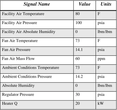
For a baseline simulation, the ACM simulation run conditions are given in Table 1. The model takes the tabulated values as inputs and performs a transient study over a set period of time. The preliminary simulation was run for 200 seconds. These variables can be dynamically changed throughout the mission simulation to better emulate the varied operating characteristics of an ACM onboard an aircraft.

(52)

39

Table 1. ACM model parameters

Signal Name

Value

Units

Facility Air Temperature 80 F Facility Air Pressure 100 psia Facility Air Absolute Humidity 0 lbm/lbm Fan Air Temperature 73 F

Fan Air Pressure 14.1 psia Fan Air Mass Flow 60 ppm Ambient Conditions Temperature 73 F Ambient Conditions Pressure 14.2 psia Absolute Humidity 0 lbm/lbm Regulator Pressure 30 psia

Heater Q 20 kW

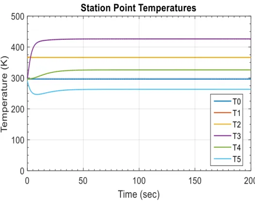
For this simulation, the ACM did not have a specified cooling load constraint that it must meet. This allowed the simulation to be run without a controller providing flexibility in studying the response of the ACM to the critical input parameters. The simulation results are the temperature, pressure and mass flow at each of the defined state points of the ACM. The simulation also captures the turbomachinery shaft speed of the ACM. The states are the compressed air within the reservoir (point 0), the air after passing through the resistive heater (point 1), air after passed through the regulating valve (point 2), air after the compressor (point 3), air after the heat exchanger (point 4), and the air after turbine (point 5). The air after the cooling turbine at point 5 is used as the coolant to the

(53)

40

load defined for the ACM. This load is representative of various load demands a typical ACM can handle such as cockpit environment cooling or avionics cooling. Figure 8 presents the temperature simulated for the ACM station points.

Figure 8. State point temperature for the ACM.

The temperature, T5, at the exit of the cooling turbine is colder than the initial

temperature. This sanity check demonstrates that the ACM is operating as a cooling mechanism. The temperatures at each state are as expected: a rise in temperature after the heater, temperature rise after compression, a drop in temperature across the heat

exchanger and the final temperature drop after the turbine. The transient period for the ACM should also be noted. Before the operating temperatures of the ACM reach steady state conditions, there are significant dynamics of the ACM that are captured.