Assimilation of Remotely Sensed Soil Moisture in the MESH Model

(1)

Assimilation of Remotely Sensed Soil Moisture

in the MESH Model

by

Xiaoyong Xu

A thesis

presented to the University of Waterloo in fulfillment of the

thesis requirement for the degree of Doctor of Philosophy

in Geography

Waterloo, Ontario, Canada, 2015

(2)

ii

AUTHOR'S DECLARATION

I hereby declare that I am the sole author of this thesis. This is a true copy of the thesis, including any required final revisions, as accepted by my examiners.

(3)

iii

Abstract

Soil moisture information is critically important to weather, climate, and hydrology forecasts since the wetness of the land strongly affects the partitioning of energy and water at the land surface. Spatially distributed soil moisture information, especially at regional, continental, and global scales, is difficult to obtain from ground-based (in situ) measurements, which are typically based upon sparse point sources in practice. Satellite microwave remote sensing can provide large-scale monitoring of surface soil moisture because microwave measurements respond to changes in the surface soil’s dielectric properties, which are strongly controlled by soil water content. With recent advances in satellite microwave soil moisture estimation, in particular the launch of the Soil Moisture and Ocean Salinity (SMOS) satellite and the Soil Moisture Active Passive (SMAP) mission, there is an increased demand for exploiting the potential of satellite microwave soil moisture observations to improve the predictive capability of hydrologic and land surface models.

In this work, an Ensemble Kalman Filter (EnKF) scheme is designed for assimilating satellite soil moisture into a land surface-hydrological model, Environment Canada’s standalone MESH to improve simulations of soil moisture. After validating the established assimilation scheme through an observing system simulation experiment (synthetic experiment), this study explores for the first time the assimilation of soil moisture retrievals, derived from SMOS, the Advanced Microwave Scanning Radiometer-Earth Observing System (AMSR-E) and the Advanced Microwave Scanning Radiometer 2 (AMSR2), in the MESH model over the Great Lakes basin. A priori

(4)

iv

rescaling on satellite retrievals (separately for each sensor) is performed by matching their cumulative distribution function (CDF) to the model surface soil moisture’s CDF, in order to reduce the satellite-model bias (systematic error) in the assimilation system that is based upon the hypothesis of unbiased errors in model and observation. The satellite retrievals, the open-loop model soil moisture (no assimilation) and the assimilation estimates are, respectively, validated against point-scale in situ soil moisture measurements in terms of the daily-spaced time series correlation coefficient (skill R).

Results show that assimilating either L-band retrievals (SMOS) or X-band retrievals (AMSR-E/AMSR2) can favorably influence the model soil moisture skill for both surface and root zone soil layers except for the cases with a small observation (retrieval) skill and a large open-loop skill. The skill improvement ΔRA-M, defined as the skill for the

assimilation soil moisture product minus the skill for the open-loop estimates, typically increases with the retrieval skill and decreases with increased open-loop skill, showing a strong dependence upon ΔRS-M, defined as the retrieval skill minus the model (open-loop)

surface soil moisture skill. The SMOS assimilation reveals that the cropped areas typically experience large ΔRA-M, consistent with a high satellite observation skill and a

low open-loop skill, while ΔRA-M is usually weak or even negative for the

forest-dominated grids due to the presence of a low retrieval skill and a high open-loop skill. The assimilation of L-band retrievals (SMOS) typically results in greater ΔRA-M than the

assimilation of X-band products (AMSR-E/AMSR2), although the sensitivity of the assimilation to the satellite retrieval capability may become progressively weaker as the

(5)

v

open-loop skill increases. The joint assimilation of L-band and X-band retrievals does not necessarily yield the best skill improvement.

As compared to previous studies, the primary contributions of this thesis are as follows. (i) This work examined the potential of latest satellite soil moisture products (SMOS and AMSR2), through data assimilation, to improve soil moisture model estimates. (ii) This work, by taking advantage of the ability of SMOS to estimate surface soil moisture underneath different vegetation types, revealed the vegetation cover modulation of satellite soil moisture assimilation. (iii) The assimilation of L-band retrievals (SMOS) was compared with the assimilation of X-band retrievals (AMSR-E/AMSR2), providing new insight into the dependence of the assimilation upon satellite retrieval capability. (iv) The influence of satellite-model skill difference ΔRS-M on skill improvement ΔRA-M was

consistently demonstrated through assimilating soil moisture retrievals derived from radiometers operating at different microwave frequencies, different vegetation cover types, and different retrieval algorithms.

(6)

vi

Acknowledgements

First and foremost, I would like to express my special thanks to my advisors, Dr. Jonathan Li and Dr. Bryan Tolson. Their invaluable guidance is gratefully acknowledged here. It was only through their support and encouragement that I have been able to accomplish my research goals proposed for this study.

I would also like to thank my supervisory committee members, Dr. Jonathan Price, Dr. William Quinton and Dr. James Craig, for their helpful comments as well as their time and support throughout my study over the years. Sincere thanks are given to the external examiner, Dr. Jing M. Chen, for his time and his helpful comments on the original version of the thesis. My appreciation also goes on to Alan Anthony, Lori McConnell, and Susie Castela for their help during my PhD study. They always answered my questions with a quick response.

I am very grateful to the European Space Agency (ESA) and the ESA Earth Observation Missions Helpdesk Team for providing the SMOS soil moisture product, to the National Snow and Ice Data Center (NSIDC) and the NASA Goddard Earth Sciences Data and Information Services Center (GES DISC) for providing access to the AMSR-E soil moisture data, to the Japan Aerospace Exploration Agency (JAXA) and the GCOM-W1 Data Providing Service for providing access to the AMSR2 soil moisture product, and to the Michigan Automated Weather Network (MAWN) and the Natural Resources Conservation Service (NRCS) for their in situ soil moisture data used in this study.

(7)

vii

Sincere thanks also go to Dr. Ralf Staebler for providing me with in situ data at Borden, to Dr. Bruce Davison and Dr. Frank Seglenieks for providing access to the MESH model code and the forcing data, to Dr. Amin Haghnegahdar for his calibration results.

This work was made possible by the facilities of the Shared Hierarchical Academic Research Computing Network (SHARCNET:www.sharcnet.ca) and Compute/Calcul Canada.

I am so thankful for the financial support through an NSERC Alexander Graham Bell Canada Graduate Scholarship-Doctoral (CGSD), a Meteorological Service of Canada Graduate Supplement Scholarship, a Research Studentship provided by Dr. Bryan Tolson, the University of Waterloo President’s Graduate Scholarship, the Dr. T.E. Unny Memorial Award, and the University of Waterloo Environmental Studies Graduate Experience Award.

Finally, I dedicate this work to my wife, my daughter, and my son for their love, patience and endless support. They are an inspiration to me every day.

Xiaoyong Xu September 2015

(8)

viii

List of Tables

Table 2.1. List of synthetic experiments... 33

Table 2.2. Error parameters for the selected forcing inputs and model variables... 35

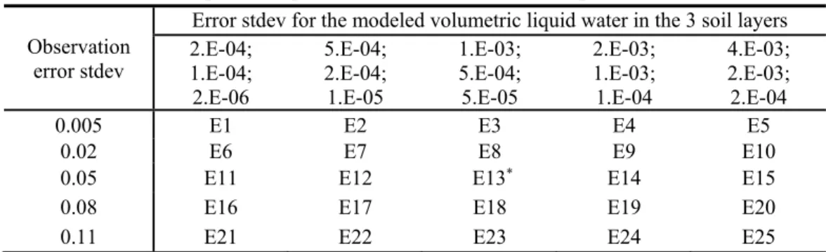
Table 2.3. Input error parameters for experiments E1-E25... 46

Table 3.1. Median and mean skill R within each grid type for soil moisture from SMOS, the open-loop model, and the assimilation, respectively... 67

Table A1. Summary of data assimilation methods ... 156

Table A2. Summary of spaceborne active microwave sensors ... 158

Table A3. Summary of spaceborne passive microwave sensors... 159

Table A4. Summary of efforts to assimilate microwave soil moisture …….…...160

(11)

xi

List of Figures

Figure 2.1. The Grouped Response Unit (GRU) approach to basin discretization and Soil

moisture and drainage representation in MESH…... 29

Figure 2.2. The Great Lakes basin ………... 30

Figure 2.3. Daily averaged surface soil moisture estimates... 36

Figure 2.4. Daily averaged root zone soil moisture estimates... 37

Figure 2.5. Soil moisture skill R from the open-loop model and the assimilation, and the skill improvement ΔR ………..………... 38

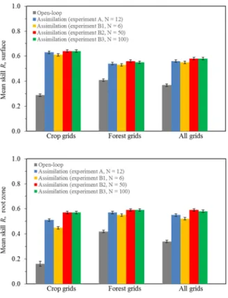
Figure 2.6. Mean soil moisture skill R for experiments A, B1, B2, and B3………... 40

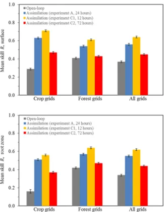
Figure 2.7. Mean soil moisture skill R for experiments A, C1, and C2 ……..….…... 42

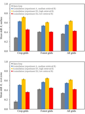
Figure 2.8. Mean soil moisture skill R for experiments A, D1, and D2 ..……..…... 44

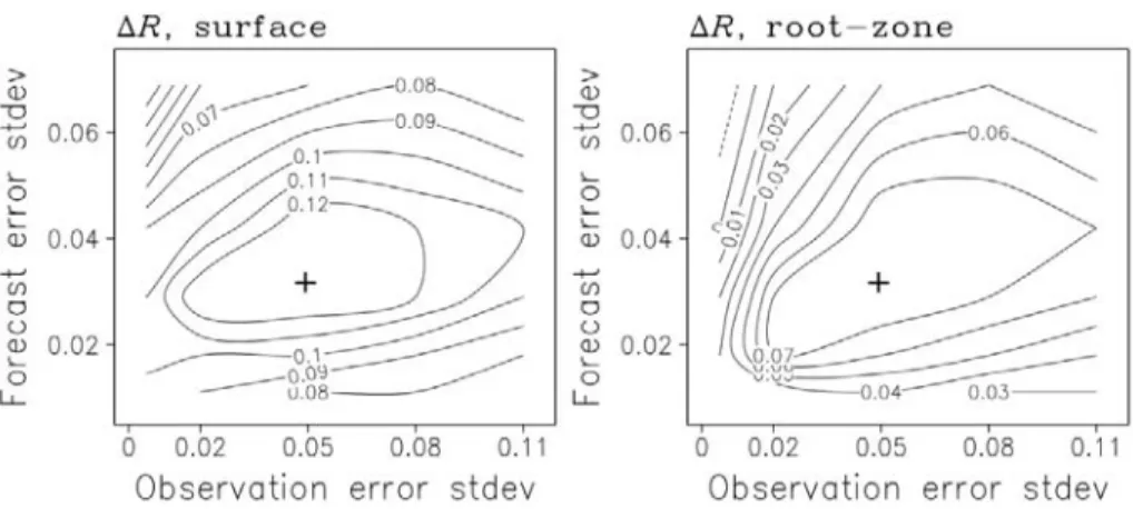
Figure 2.9. Skill improvement ΔR as a function of the forecast and observation error standard deviations... 47

Figure 3.1. Vegetation types over the Great Lakes basin and location of in situ stations for soil moisture measurements...57

Figure 3.2. Comparison of volumetric water content daily time sequences for four pairs of MAWN sites…... 63

Figure 3.3. SMOS soil moisture skill………... 66

Figure 3.4. Skill for surface soil moisture from the open-loop model and the assimilation, and the skill improvement over four individual years... 72

Figure 3.5. Similar to Fig. 3.4, but for root-zone soil moisture………... 75

Figure 3.6. Skill improvement ΔRA-M against ΔRS-M ... 76

Figure 3.7. Skill improvement ΔRA-S, defined as the skill for the surface soil moisture assimilation product minus the SMOS observation skill…………... 81

Figure 4.1. Retrieval skill for AMSR-E NSIDC product and AMSR-E LPRM product over years 2009, 2010, and 2011, respectively……...102

Figure 4.2. Skill for surface soil moisture from the open-loop model, the assimilation of NSIDC and LPRM, and the skill improvement ΔRA-M... 104

(12)

xii

Figure 4.4. Mean soil moisture skill R for the AMSR-E retrievals, the open-loop model,

and the assimilation estimates...108 Figure 4.5. Skill improvement ΔRA-M against ΔRS-M, derived from the assimilation of

AMSR-E……….. 111 Figure 4.6. Mean soil moisture skill R for the satellite retrievals, the open-loop model,

and the assimilation estimates...114 Figure 5.1. Location of validation sites. ………... 122 Figure 5.2. Scatterplot of SMOS vs AMSR2 for the retrieval skill and the number of days with available retrieval data. ………... 125 Figure 5.3. Scatterplot of SMOS vs AMSR2 for the assimilation skill and the skill improvement ………... 126 Figure 5.4. Skill improvement ΔRA-M as a function of the retrieval skill and open loop

skill………... 128 Figure 5.5. Mean soil moisture skill R for the satellite retrievals, the open-loop model,

(13)

1

CHAPTER 1 Introduction

1.1 Background

Changes in the spatial and temporal distribution of water resources are expected to play a major role in driving the impacts of climate and global change on human settlements and infrastructure (Bates et al., 2008). The monitoring and prediction of water resources under climate change typically rely on in situ and remote sensing observations, and reliable numerical modeling systems. In situ observations of hydrological conditions (e.g. precipitation, snow, soil moisture and evapotranspiration) are generally based upon uneven point sources, and have limited and sparse spatial coverage except in developed areas or well-designed field experiments. Satellite remote sensing offers better geographical coverage and holds the capability to provide large-scale spatially distributed measurements. A variety of hydrology-related variables, such as precipitation, snow cover, snow water equivalent, surface soil moisture, land surface temperature, leaf area index, and evapotranspiration, can be estimated using remote sensing (see the review papers by Rango, 1994; Tang et al., 2009; Zheng and Moskal, 2009; Li et al., 2009; Wang and Qu, 2009; Dietz et al., 2012). Overall, however, the temporal and/or spatial coverage of remote sensing measurements is still not sufficient for many practical applications because remote sensing provides only instantaneous values of the object within the sampled area (instantaneous field of view, IFOV) at the observing time. Additionally, satellite remote sensing cannot measure the information (e.g. soil water content) below a thin surface layer.

(14)

2

On the other hand, land surface and hydrological model simulations, in particular for physically-based distributed models, allow for the estimation and prediction of hydrologic conditions at desired spatial and temporal scales. In practice, however, land surface and hydrologic modeling is often difficult because we have neither a perfect forecast model nor perfect forcing data. The accuracy of state estimation suffers from uncertainties in forcing fields and deficiencies in model physics and/or parameters. To improve the model simulations, one may constrain the model forecasted state in time with observations. A simplistic method is a direct insertion, which uses observations to directly replace the corresponding model predictions at measurement times. Nevertheless, observation errors, which always exist but are ignored in the direct insertion method, could degrade the state estimation (Additionally, a direct insertion is applicable only when the model variable is directly connected to the observed variable). To circumvent these problems, observations should be integrated into the model dynamical framework by taking into account both the model forecast and observation errors. The effects on the state estimation (analysis) of the model and observations will be controlled by their respective error statistics. This allows a state estimation superior to either the model forecast or the observation alone to be produced. Meanwhile, the observed information can, by means of consistency constraints based upon the time evolution and physical properties of the system, spread to times and locations that are not directly observed. This is the basic concept of data assimilation.

Soil moisture information is critical to the monitoring and modeling of climate and global changes (e.g. Zhang and Frederiksen, 2003). As a reservoir for evapotranspiration, soil moisture has an important controlling on the partitioning of energy fluxes between

(15)

3

latent and sensible forms at the land surface. In the presence of extensive soil moisture anomalies, land surface fluxes may modulate the large-scale atmospheric circulation during the summer (e.g. Wolfson et al., 1987; Fischer et al. 2007). Soil moisture affects precipitation across a range of spatial and temporal scales (e.g. Talyor et al., 2012; Collow et al., 2014). Soil moisture regulates the partitioning of rainfall into runoff (surface discharge) and infiltration on land surfaces, and therefore has significant impacts upon streamflow forecasting in rainfall-runoff models (e.g., Maurer and Lettenmaier, 2003; Berg and Mulroy, 2006). Traditionally, soil moisture can be in situ measured using a gravimetric method or ground-based sensors (probe, time domain reflectometry, ground penetrating radar, etc.). In situ measurements typically serve as the “ground truth”, but spatially distributed soil moisture information, especially at regional, continental, or global scales, is difficult to estimate from in situ measurements that are typically based upon sparse point sources in practice. Satellite microwave remote sensing (e.g. Jackson, 1997; Bindlish et al., 2003; Njoku et al., 2003; Owe et al., 2008; Kerr et al., 2012; Entekhabi, et al., 2010a) holds the ability to provide a large-scale monitoring of surface soil moisture because microwave measurements respond to changes in the surface soil’s dielectric properties, which are strongly controlled by soil water content. Over the past decade, satellite microwave soil moisture retrievals have shown great potential to improve the predictive skill of land surface and hydrologic models, especially through data assimilation techniques (see section 1.2.3). In a data assimilation system, near-surface soil moisture information derived from satellite microwave measurements can spread to deeper soil layers that cannot be directly measured by satellite microwave sensors. Furthermore, soil moisture observations from

(16)

4

different satellite platforms can, through data assimilation, be merged within the same model framework to yield a single optimal soil moisture estimation.

With recent advances in satellite microwave soil moisture estimation, in particular the launches of the Soil Moisture and Ocean Salinity (SMOS) satellite and the Soil Moisture Active Passive (SMAP) mission, there is an increased demand for exploiting the potential of satellite microwave soil moisture observations to improve the predictive capability of hydrologic and land surface models. This doctoral study aims to assimilate satellite microwave soil moisture observations into a distributed land surface-hydrological model and to demonstrate the contribution of the assimilation to the model soil moisture estimates for both surface and root zone soil layers. The improved soil moisture estimates resulting from the assimilation would benefit weather and climate forecast initializations. In the long term, outcomes of this study can improve the monitoring and prediction of water recourses under climate change, thus providing better guidance for water resource related applications and management.

1.2 Literature review

1.2.1 Data assimilation methods

In essence, data assimilation aims to estimate a posterior probability density function (PDF) of the model state given observations from one or more sources (Bayes' theorem). A great number of data assimilation methods have been developed for land and hydrologic

(17)

5

applications (Table A1). In most cases, we assume that the model and observation errors are Gaussian, and thus the analysis problem can be resolved with either a maximum-likelihood estimator (e.g. variational assimilation methods) or a variance minimizing estimator (e.g. Kalman filter, KF; extended Kalman filter, EKF; or ensemble Kalman filter, EnKF). A variational assimilation method (e.g. three-dimensional variational assimilation, 3DVAR; or four-dimensional variational assimilation, 4DVAR) seeks the state with the maximum likelihood by minimizing a cost function that contains, at least, a background term, a measure of the misfit between the model state x (unknown) and the forecast background (a priori sate), and an observation term, a measure of the misfit between x and observations. In contrast, the Kalman Filter (KF) and its variants (EKF, EnKF) directly compute the Kalman gain matrix and derive the analysis state based upon the analysis equation, which is supposed to ensure minimum analysis error variances. In the KF and the EKF, an additional error covariance equation is utilized to propagate the model forecast error information while the EnKF uses a Monte Carlo sampling (an ensemble of model states and an ensemble of perturbed observations) to estimate error statistics and the evolution of the model forecast error information is implemented by integrating the ensemble of model states forward in time. As compared to the variational methods, a variance minimizing estimator is relatively easy to implement since an adjoint version of the forecast model is not required. These assimilation techniques are further detailed as below.

(18)

6 a. Variational data assimilation

A variational method does not directly compute the analysis state. Instead, it seeks an equivalent solution to the analysis problem by minimizing a predefined cost function, given by

(1.1)

where xb_{represents the background (a priori) model state,}_Y_{is the observation,}_B_and_R

denote the respective error covariances of xb_and_Y_._H_{is a linear or linearized observation}

operator, which relates the model state variable to the observed variable. The superscript T denotes the transpose of the matrix. The first right-hand-side term of (1.1) is called the background term, which is an objective measure of the misfit between the state x (unknown) and the background model state xb_{. The second right-hand-side term of (1.1) is}

the observation term, which quantifies the misfit between x and the observation Y. If multiple observation types (assuming the observation errors are uncorrelated) are to be assimilated, the observation term in (1.1) can be broken down into multiple terms, each observation type having its own observation term. Additionally, to impose additional weak constraints, more terms (e.g. the penalty term) can be added to the right-hand-side of (1.1). In practice, a suitable descent algorithm is needed to iteratively search for an approximate solution to the minimization of J(x). At each iteration step, a new estimation of x is made to produce as possible as great reduction in J(x). The search direction (descent direction) is determined based upon the local slope, i.e. the gradient of the cost function. When the minimum of J(x) is found, the corresponding x is the optimal analysis state. In a realistic

(19)

7

application, only a small number of iterations are performed to ease the computational burden. The cost function in (1.1) can be employed to different spatial dimensions, such as one-dimensional variational assimilation 1DVAR (e.g. assimilation of satellite sounding data) and three-dimensional variational assimilation 3DVAR (e.g. a global assimilation analysis of the 3D meteorological fields).

Further, if the minimization is extended to the time domain, it is called the four-dimensional variational analysis (4DVAR). The corresponding cost function is defined as

∑ (1.2)

In (1.2), the observation term of the cost function contains the differences between the state x and observation Y over a time interval (t0 to tn), while the background term is defined

only at initial time t0. The basic idea of 4DVAR is to seek an optimal state x at t0 (i.e. initial

condition ) to yield (through the forward integration of the model assuming the model is perfect) the sequence of optimal states (ti represent the observation time, i = 0, …,

n), which will lead to the minimum of the cost function defined in (1.2). The minimization procedure of the 4DVAR cost function can be summarized as follows. (i) The forecast model is integrated forward (from t0 to tn) with a first guess of the initial condition to

produce the forecast state at each observation time ti over the time interval, and the cost

function (1.2) is calculated. (ii) The adjoint model of the forecast model (a conjugate transpose of the tangent linear model of the forecast model) is integrated backward to the beginning of the time window (from tn to t0), and the gradient of the cost function with

(20)

8

convergence criterion is met or not; if the convergence criterion is not met, the initial condition of the forward model is adjusted based upon the descent direction, which is estimated using the gradient of the cost function as calculated in (ii). (iv) Repeat the steps (i) to (iii) until the convergence criterion is met and the optimal forecast trajectory is determined. To perform 4DVAR, the construction of the adjoint model of the forecast model is required, and could be difficult if the forecast model is highly nonlinear and complex. In practice, some approximations have to be adopted when deriving the adjoint model (e.g. ignoring moisture physical processes in the adjoint atmospheric model) to limit possible numerical instability arising from nonlinear processes. The readers are referred to the relevant references (e.g., Talagrand and Courtier, 1987) for more details on the minimization of the cost function, the adjoint equations, and the descent algorithms

Note that 4DVAR using the cost function defined in (1.2) deals with only the uncertainty in the model initial condition, and ignores deficiencies in the model physics and parameters (i.e. assuming that the model is perfect). This is the so-called strong-constraint, i.e. the sequence of model states over the time interval must completely comply with the forecast equations. To impose external weak constraints to deals with other errors such as the deficiencies in the model physics and noises in the forcing fields, additional terms can be placed to the right-hand-side of (1.2) (e.g. Reichle et al. 2001a). In 4DVAR, all the observations distributed in this interval are assimilated simultaneously, and the observational information is propagated not only from the past into the future but also from the future into the past. That is to say, the state estimation over the assimilation interval

(21)

9

(time window) is influenced by all the observations distributed in this interval. Therefore, 4DVAR is a typical representative of the smoothing (or batch) algorithm.

b. Kalman Filter and its variants

The Kalman Filter (KF) and its various variants (extended Kalman Filter, EKF; ensemble Kalman Filter, EnKF) are typical ‘filtering’ (or sequential) assimilation techniques. As compared to the ‘smoothing’ algorithm 4DVAR, the implementation of sequential ‘filtering’ technologies is relatively easy since an adjoint version of the forecast model is not required, and therefore makes themselves more attractive for land surface and hydrologic data assimilation. In the traditional KF, each assimilation cycle consists of two steps: a forecast step and an analysis step. In the forecast step, the forecast model is integrated forward in time (from an initial or analysis state) with an additional error covariance equation to propagate error information:

, (1.3) (1.4) where x and P denote the model state and the associated error covariance matrix, respectively; the subscript k denotes the time index; the superscripts f and a represent forecast and analysis, respectively. u denotes uncertainties in the model (errors in forcing data and/or deficiencies in model parameters/physics). M denotes the model operator and Q stands for the model error.

(22)

10

In the analysis step (time index k omitted) the new observation is used to adjust the current forecast estimation. The analysis equation of the KF is given by,

(1.5) Meanwhile, the error covariance matrix can be updated using

(1.6) Starting from the updated state xa_{and error estimation}_Pa_{, equations (1.3) and (1.4) are then}

integrated forward to produce the forecasted and for the next observation. As such, the observational information is accumulated into the model state in a sequential manner.

The KF is valid only for linear systems. Its variants have been developed to solve the optimal estimation problem for nonlinear systems. The EKF still uses equations (1.3)-(1.6) but with M in equation (1.3) being a nonlinear operator and M in (1.4) being its linearized version. Equation (1.4) indicates that the linear KF and its nonlinear variant, the Extended Kalman filter (EKF), explicitly compute and propagate the error statistics. In practice, the full error covariances are difficult or impossible to be directly estimated due to an expensive computational cost and insufficient error information, especially for large-scale applications. Additionally, the use of a linearized and approximate error covariance equation may cause the EKF to fail to track the state space in a strongly nonlinear system since higher-order components are ignored. To this end, Evensen (1994) proposed the Ensemble Kalman filter (EnKF) where the Fokker-Planck equation defining the time evolution of the model state’s probability density was solved using a Monte Carlo method. The probability density function (PDF) of the model state is represented using an ensemble where the mean is the best estimate (Gaussian assumption) and the ensemble spread defines

(23)

11

the error variance. The measurement errors are represented using another ensemble with the mean equal to zero. The evolution of the forecast error statistics is implicit in ensemble forecasts. In contrast to the EKF, the error evolution is fully nonlinear in the EnKF but with lower rank (finite ensemble size).

Similar to the KF and EKF, the EnKF sequentially conducts a forecast step and an analysis step. In the forecast step, the ensemble of model states, generated by a Monte Carlo method, are integrated forward in time, expressed as

, , , , 1, … , (1.7)

where M denotes the model operator, x denotes the model state, uj denotes uncertainties in

the model (perturbations to the forcing data or deficiencies in model parameters/physics), the superscripts f and a represent forecast and analyzed state, respectively; the subscript k denotes the time index, and j is the ensemble member index, counting from 1 to the number of model state ensemble N.

In the analysis step (time index k omitted), the Kalman gain K is estimated from the forecast and measurement error covariances and each forecast ensemble member is then updated according to the Kalman analysis equation.

, , , (1.8) 1, … , (1.9)

where σ denotes the covariance between two vectors, and denote the forecast and analysis model state of the jth ensemble member. and represent the perturbed

(24)

12

observation and the corresponding model prediction. , and ɛ represents the ensembles of , , and observation errors, respectively. The best estimation is represented by the analysis ensemble mean. With an infinite ensemble size the EnKF will yield exactly the same analysis as the EKF.

1.2.2 Microwave remote sensing for surface soil moisture estimation

Soil moisture is an important variable for numerical weather, climate, and hydrologic forecasts. This is because soil moisture plays a crucial role in hydrological cycle by controlling the partitioning of water and energy fluxes at the land surface and the moisture exchanges at the soil-vegetation-atmosphere interface. Surface soil moisture can be estimated using various remote sensing instruments including microwave, optical, and thermal infrared sensors (see a review by Wang and Qu, 2009). Microwave techniques are of particular value for surface soil moisture estimation because microwave measurements are sensitive to changes in the soil dielectric properties, which are strongly controlled by soil water content. Liquid water has a very high dielectric constant (~80-90 at 0-20ºC) while the dielectric constant is very low (only ~ 4) for dry soil. Such a high contrast between the dielectric constants of wet and dry soils forms the basis for deriving soil moisture information from microwave remote sensing measurements. Over the past decades, both active and passive microwave technologies have been developed for surface soil moisture estimation (Jackson, 2005). Passive microwave sensors (radiometers) measure the natural thermal radiation emitted from the soil (brightness temperature), while active microwave sensors (radars) emit energy to the land surface and observe the radiation backscattered by

(25)

13

the soil (backscattering coefficient). The mixed dielectric constant of the soil’s constituents can be retrieved based upon the acquired brightness temperatures or backscattering coefficients. Ultimately, soil water content can be estimated by means of a soil dielectric mixing model.

Tables A2 and A3 summarize the representative microwave sensors, respectively, for satellite active and passive soil moisture measurements. For spaceborne active measurements, the ESA Remote Sensing Satellite (ERS) Synthetic Aperture Radar (SAR) and Scatterometer (SCAT), the Canadian RADARSAT series (e.g. Merzouki et al., 2011), and the Advanced Scatterometer (ASCAT) onboard the Meteorological Operational (Metop) satellite (e.g., Bartalis et al., 2007; Albergel et al., 2009), successor of the SCAT, have played important roles within the past decades; while passive microwave observations typically relied upon the Special Sensor Microwave Imager (SSM/I) (e.g. Jackson, 1997), the Scanning Multichannel Microwave Radiometer (SMMR) (e.g. Reichle and Koster, 2005; Owe et al., 2008), the Tropical Rainfall Measuring Mission Microwave Imager (TMI) (e.g. Bindlish et al., 2003), the Advanced Microwave Scanning Radiometer-Earth Observing System (AMSR-E) (e.g. Njoku et al., 2003; Njoku and Chan, 2006), the Advanced Microwave Scanning Radiometer 2 (AMSR2), or the Microwave Imaging Radiometer with Aperture Synthesis (MIRAS) onboard the Soil Moisture and Ocean Salinity (SMOS) satellite (Kerr et al., 2001; 2010; 2012). In particular, the SMOS mission and the newly launched (January 2015) Soil Moisture Active Passive (SMAP) mission (Entekhabi et al., 2010a) were designed exclusively for soil moisture monitoring. The L-band (1.3 or 1.4 GHz) sensors carried by the two satellites have stronger penetration of soil

(26)

14

and vegetation than those operating at higher frequencies (e.g. X or C-band), and thus greatly enhance our capability to map large-scale surface soil moisture.

There is usually an inverse relationship between a sensor’s temporal frequency and spatial resolution. The active SAR technology is able to scan the land at a high spatial resolution, but the revisit time is very long. Passive microwave sensors onboard polar-orbiting satellites offer a higher time resolution (revisit per 1-3 days) due to their wide swaths, but generally result in relatively coarse spatial samplings. Overall, soil moisture retrieval is challenging for active microwave sensors because radar signal is highly sensitive to local features of the soil surface (surface roughness, topography, vegetation, etc.), while passive microwave soil moisture products are usually more reliable due to higher signal-to-noise ratio and mature retrieval algorithms. Microwave sensors measure only the soil moisture within a near-surface layer. The soil thickness measured increases with the wavelength (approximately several tenths of the wavelength). For bare soil, the penetration depth is about 3-5 cm for L-band (1-2 GHz) sensors (e.g. SMOS), and only ~1-1.5 cm for C (4-8 GHz) or X (8-12 GHz) band measurements (e.g. AMSR-E). Soil moisture estimation using microwave sensors is subject to vegetation effects. Where there is a vegetation cover, the radiation emitted or backscattered from the soil will be attenuated owing to the scattering and absorption by vegetation canopy. The magnitude of the vegetation attenuation increases with the sensor frequency and the vegetation density. Hence soil moisture retrieval at high microwave frequencies (> 5-6 GHz) is valid only for bare soil or sparely vegetated regions. Vegetation cover impacts upon sensors operating at low frequencies are less pronounced because the latter can penetrate moderately dense

(27)

15

canopies. For example, L-band sensors (e.g. SMOS) can provide reliable measurements over a wide range of vegetation cover (biomass ≤ 5 kg/m2_).

1.2.3 Assimilation of microwave remotely-sensed soil moisture in land surface and hydrological models

Thanks to the development of data assimilation technologies and the launches of various passive and active microwave sensor systems, there has been an intensive global research effort to assimilate microwave remote sensing soil moisture information into land surface or hydrological models within the past few decades (Table A4). The studies generally can be divided into three major categories as follows.

(i) A direct assimilation of microwave brightness temperatures in land surface models (LSM). A series of synthetic assimilation experiments based upon the 1997 Southern Great Plains hydrology experiment demonstrated that a direct assimilation of microwave brightness temperature data in LSMs could provide reliable soil moisture estimates (e.g. Reichle et al., 2001a, 2001b, 2002b). In practical application, Margulis et al. (2002) used the EnKF method to assimilate airborne Electronically Steered Thinned Array Radiometer (ESTAR) 1.4 GHz surface brightness temperature measurements during SGP97 into Noah LSM. Crow and Wood (2003) conducted similar assimilation experiments with the TOPMODEL-Based Land Surface-Atmosphere Transfer Scheme (TOPLATS) model. Their results showed that the assimilation of ESTAR brightness temperature measurements led to good soil moisture estimates not only in the surface layer but also for root zone.

(28)

16

Mattia et al. (2009) demonstrated that high spatial resolution surface soil moisture could be estimated through an integration of SAR data and hydrologic modeling with a constrained minimization technique. In their SAR retrieval algorithm, the hydrological model provided the background information about soil moisture at coarse spatial resolution based on the Antecedent Precipitation Index (API) approach.

(ii) Assimilation of microwave soil moisture retrievals in LSM. As one of the pioneer studies, for instance, Houser et al. (1998) incorporated soil moisture derived from the NASA L-band (1-2 GHz) push broom microwave radiometer (PBMR) mounted on a NASA C-130 aircraft into the hydrologic model TOPLATS with several assimilation schemes. Results showed that all the assimilation schemes could produce substantial improvements in the model surface soil moisture simulations. Reichle and Koster (2005) assimilated the surface soil moisture retrievals from SMMR into the NASA Catchment Land Surface Model (CLSM) with the EnKF method. Reichle et al. (2007) assimilated both SMMR and AMSR-E soil moisture retrievals into CLSM. The assimilation led to overall improvements, relative to either the model estimates or satellite retrievals alone, in terms of soil moisture anomaly time series correlation with in situ measurements. In Draper et al. (2009a), the Extended Kalman Filter (EKF) method was used to assimilate the surface soil moisture derived from AMSR-E C-band brightness temperature measurements with the Land Parameter Retrieval Model (LPRM) into the Interactions between Surface, Biosphere, and Atmosphere (ISBA) land model. The introduction of AMSR-E soil moisture did yield substantial analysis increments (changes in the model estimate between before and after the implementation of the analysis equation) for both surface and

(29)

root-17

zone soil moisture, although the assimilation estimates were not validated against real in situ observations. Liu et al. (2011) showed that the assimilation of AMSR-E soil moisture was as efficient as the precipitation corrections for enhancing the model skill for soil moisture estimation (anomaly time series correlation coefficient with in situ measurements). The study assessed the contributions of two AMSR-E soil moisture products (June 2002 to July 2009), the NASA standard algorithm product archived at the National Snow and Ice Data Center (NSIDC) and the LPRM-derived AMSR-E soil moisture. The assimilation of LPRM product led to larger soil moisture skill improvement than the NSIDC product. Draper et al. (2012) suggested that the CLSM model soil moisture skill could be improved through the assimilation of either AMSR-E or ASCAT soil moisture retrievals. A joint assimilation of the two sensor products could produce the best soil moisture skill. Due to the bias (systematic error) between satellite retrievals and the model estimates, a priori rescaling on satellite retrievals (the cumulative distribution function (CDF) matching) was applied during the aforementioned efforts. Li et al. (2012) assimilated AMSR-E soil moisture retrievals (derived from the X-band brightness temperatures using single-channel algorithm), without a priori scaling, into the Noah land surface model. Their work was motivated by the assumption that the mean value of satellite retrievals have potential contribution to improving the model mean values of soil moisture. Although the study observed the improved soil moisture estimates (as indicated by reduced bias and root-mean-square-error against in situ measurements), especially for the mass conservation scheme, the analysis typically made systematic corrections to the model soil moisture estimation (a clear symptom of bias in the assimilation). This means that a

(30)

18

satellite-model bias removal is an indispensable part in a bias-blind assimilation system (i.e. correcting random errors only).

(iii) Assimilation of microwave soil moisture observations in runoff models. During a flooding event, the affected areas are usually characterized by wet pre-storm soil moisture conditions. This provides an opportunity to improve streamflow forecasts by identifying antecedent soil moisture conditions with microwave remote sensing observations. Pauwels et al. (2002) improved the simulated hydrographs in TOPLATS through the assimilation of ERS SAR soil moisture estimates using a statistical correction approach. Francois et al. (2003) applied the EKF method to assimilating soil moisture retrieved from ERS-1 SAR into a lumped rainfall-runoff model. The study demonstrated that the sequential assimilation of SAR data had the potential to improve the runoff simulations. Jacobs et al. (2003) introduced the surface soil moisture observed by ESTAR during the SGP97 hydrology experiment into a lumped rainfall-runoff model. The ESTAR soil moisture retrievals were used to represent antecedent soil moisture conditions and to update the curve numbers and the runoff predictions based upon a strong correlation between the curve number and soil moisture in the Soil Conservation Service (SCS) curve number method. Results showed an enhancement in runoff forecasts for the watersheds at different spatial scales. Regarding the earlier studies of assimilating ERS SAR soil moisture retrievals into hydrological models, we refer the readers to a review paper by Loumagne et al. (2001). Crow et al. (2005) suggested that the predictive capability of land surface’s response to precipitation was enhanced when TMI-derived surface soil moisture was sequentially assimilated into an API model. Brocca et al. (2010) explored the impact on

(31)

19

flood forecasting of assimilating ASCAT-based soil wetness index in a rainfall-runoff model. Results revealed that the assimilation of the ASCAT soil moisture estimates via a simple nudging scheme led to an enhancement in runoff predictions. Crow and Ryu (2009) proposed a new assimilation scheme in which remotely-sensed surface soil moisture measurements were employed to simultaneously adjust both antecedent soil moisture and rainfall accumulations during hydrological modeling. Their work was motivated by the additional capability of soil moisture data to filter errors contained in satellite-based rainfall products (Crow and Zhan, 2007; Crow et al., 2009). Preliminary results indicated that the new approach outperformed those schemes which considering only the calibration of antecedent wetness conditions.

1.2.4 Research gaps and recommendations

The encouraging results warrant further research efforts in this field. In particular, with the launches of SMOS and SMAP, our capability to map large-scale soil moisture by microwave remote sensing is progressively enhanced, which will surely trigger more research efforts in satellite soil moisture assimilation over the next decade. The upcoming research efforts should cover the following aspects: (i) assimilation of new L-band soil moisture products (mainly from SMOS and SMAP). Until recently satellite soil moisture measurements at X (8-12 GHz) and C (4-8 GHz) bands (e.g. SMMR, AMSR-E, TMI, ASCAT, or SAR) have been dominant in land/hydrologic data assimilation applications. The launches of SMOS and SMAP have opened up new opportunities for L-band soil moisture assimilation. Assimilation of SMOS and SMAP soil moisture is more attractive

(32)

20

because the ability of SMOS and SMAP to measure surface soil moisture for a wide range of vegetation covers is clearly of advantage for assessing the vegetation modulation of the assimilation. (ii) Comparison between L-band and X-band (or C-band) soil moisture measurements for land data assimilation. In land/hydrologic data assimilation applications, to date, there has been a lack of comparative studies of multi-sensor soil moisture products, especially from different microwave bands, which represent different retrieval capabilities. At the moment, satellite soil moisture estimates for the same location and within the same time period can be available for both L-band sensors (e.g. SMOS, SMAP) and X-band (or C-band) measurements (e.g. AMSR-E/AMSR2, ASCAT). Their comparison for land data assimilation and even their joint assimilation will offer further insight into the dependence of the assimilation upon the satellite observation skill. (iii) Application of nonlinear/non-Gaussian assimilation approaches. Current methods (e.g. KF, EKF, EnKF, and 4DVAR) for assimilating satellite soil moisture are typically based upon the assumption of Gaussian error statistics. For a nonlinear system with the error statistics far from Gaussian, to take into account the influence of skewed PDF, general nonlinear/non-Gaussian filters (e.g. the Particle Filter) should be applied.

1.3 Research objectives

The overall goal of this research is to exploit the potential of satellite microwave soil moisture observations to improve the predictive capability of hydrologic and land surface models. The limited research objectives are set as follows: 1) to develop nonlinear filter algorithms for assimilation of satellite soil moisture in a distributed land

(33)

surface-21

hydrological model; 2) to explore the impact of satellite microwave soil moisture, through a data assimilation scheme, upon the model soil moisture estimates; and 3) to advance our understanding of the satellite observation skill and vegetation cover impacts on the assimilation results. In the long term, this study aims to improve the monitoring and prediction of water recourses under climate change, thus providing better guidance for water resource related applications and management.

As part of an operational forecasting system developed at Environment Canada, the modelling system called Modélisation Environmentale-Surface et Hydrologie (MESH) provides a flexible framework for coupling land surface schemes, a hydrological model, and an atmospheric model (Pietroniro et al., 2007). In this thesis, the ensemble Kalman filter (EnKF) is utilized to assimilate SMOS, AMSR-E and AMSR2 soil moisture retrievals into the standalone version of MESH in which CLASS, the Canadian Land Surface Scheme, is coupled with a distributed hydrological model over the Great Lakes basin. This is the first study to assimilate these satellite retrievals in the MESH model. This work will address the following questions. Fundamentally, how will satellite retrievals of surface soil moisture, through data assimilation, impact the MESH model soil moisture estimates? Next, how does the vegetation cover modulate the assimilation performance? Finally, how important is the satellite observation skill to the assimilation estimates? To this end, the main contents of this thesis include: 1) to equip the MESH model with the EnKF scheme for assimilation of satellite soil moisture retrievals; 2) to validate the performance of the established assimilation system through observing system simulation experiments (synthetic experiments) and assimilation of real satellite retrievals; 3) to reveal the

(34)

22

vegetation modulation of assimilation by taking advantage of the ability of L-band senor (SMOS) to measure surface soil moisture for a wide range of vegetation covers; 4) to compare L-band retrievals (SMOS) and X-band retrievals (AMSRE/AMSR2) in the same assimilation system.

In this thesis, the EnKF method is used because (i) as compared to the variational methods, the EnKF is relatively easy to implement since an adjoint version (a conjugate transpose of the tangent linear model) of the forecast model is not required; (ii) estimation of full error covariances (as used in the EKF) is not required in the EnKF, and the model and measurement error variances are defined by the ensemble spreading (although the input error parameters may need to be specified based upon empirical statistics or to be adaptively tuned); and (iii) the EnKF is an ensemble-based method and thus can be easily merged into the existing ensemble forecasting system in use with Environment Canada.

The focus of this work is upon improvement in soil moisture estimates rather than in hydrologic forecasts (e.g. in the range of a few days). The soil moisture estimates (satellite, the model, and the assimilation) are quantitatively evaluated using the correlation R metric of skill, which is defined as the daily time series correlation with point-scale in situ soil moisture measurements. Note that satellite soil moisture retrievals are instantaneous observations (typically once every 1-3 days for this study). The satellite soil moisture skill R is computed only over the days with available satellite data, whereas the model and assimilation skill R values are obtained based upon the complete model simulation time series (except for snow covered or frozen soil periods) rather than using the soil moisture

(35)

23

estimates only at satellite observation (i.e. assimilation) times. The absolute error measure (e.g. the root-mean-square error (RMSE) metric) is not applicable here because (1) point soil moisture measurement typically contain substantial sampling errors in terms of absolute magnitude (Crow et al., 2012), while the temporal variability of soil moisture observed by point measurements used in this study is often spatially representative; and (2) the absolute magnitude of the soil moisture assimilation product is meaningless since the satellite retrievals are rescaled prior to the assimilation (Reichle et al., 2007). However, notice that through a percentile-based transformation (e.g., Entekhabi et al. 2010b) the time variations of soil moisture can be scaled to the soil moisture initial conditions of weather and climate models, while any bias (systematic error) in the soil moisture product can be scaled out (e.g. Zhang and Frederiksen, 2003). Therefore, the resulting soil moisture assimilation product can benefit weather and climate forecast initializations as long as the time variability of soil moisture is better captured.

The thesis is organized as follows. Chapter 2 describes the establishment of the EnKF assimilation scheme for the MESH model and examines the performance of the assimilation system under different conditions through the Observing System Simulation Experiment (synthetic experiments). Chapter 3 is focused upon the assimilation of SMOS soil moisture retrievals (2010-2013). Chapter 4 presents the assimilation of two AMSR-E soil moisture products (2003-2011) and their comparison with the assimilation of SMOS. Chapter 5 compares the assimilation of AMSR2 and SMOS retrievals for year 2013. The main conclusions and contributions of this thesis are presented in Chapter 6.

(36)

24

1.4 Statement of manuscript submission and author contributions

This doctoral thesis is comprised of the following published and submitted papers in refereed journals.

[1] Chapter 2: Xu, X., B. A. Tolson, and J. Li (2015). Assimilation of satellite soil moisture data in the MESH model with the Ensemble Kalman filter: Synthetic experiments. Journal of Water Resources Planning and Management, under review (Manuscript number WRENG-2247).

[2] Chapter 3: Xu, X., B. A. Tolson, J. Li, R. M. Staebler, F. Seglenieks, A. Haghnegahdar, and B. Davison (2015). Assimilation of SMOS soil moisture over the Great Lakes basin. Remote Sensing of Environment, 169: 163-175, doi:10.1016/j.rse.2015.08.017. [3] Chapters 4 & 5: Xu, X., B. A. Tolson, J. Li, B. Davison, and A. Haghnegahdar (2015).

Comparison of X-band and L-band soil moisture retrievals for land data assimilation. Remote Sensing of Environment, under review (Manuscript number RSE-D-15-00783).

For all manuscripts, X. Xu conceived the study, performed the analysis and wrote the paper. B.A. Tolson and J. Li provided guidance and edited the manuscripts. R. M. Staebler provided in situ soil moisture data for paper [2]. B. Davison and F. Seglenieks provided access to the MESH model code and the forcing data. A. Haghnegahdar provided his MESH calibration results.

(37)

25

CHAPTER 2 Synthetic Assimilation Experiments

2.1 Introduction

Soil moisture plays a crucial role in the Earth’s energy and water cycles. Specifically, (i) soil moisture is a key state variable linking the land surface and the atmosphere. Soil moisture can bring a significant component of memory into the soil-atmosphere system through an integration of precipitation and evaporation processes over time scales of days to weeks. The memory has an important influence on the surface saturation and the forecasting of flooding events; (ii) Soil moisture, as a reservoir for evapotranspiration, controls the partitioning of the incoming radiative energy between latent and sensible heat fluxes at the land surface. The soil water content greatly impacts the evaporative proportion from the land surface and the transpiration from the root zone, which in turn control the ground sensible heat fluxes; (iii) Soil moisture regulates the partitioning of rainfall into runoff (surface discharge) and infiltration at the land surface. In particular, accurate specification of antecedent (pre-storm) soil moisture conditions is crucial to flooding forecasts; (iv) Accurate initialization of soil moisture is critical to numerical weather and climate predictions. For example, in the presence of extensive soil moisture anomalies, land surface fluxes can modulate the large-scale atmospheric circulations during the summer, thus influencing short- and long-term precipitation and temperature patterns.

(38)

26

In situ measurements, which are typically based upon sparse point sources, cannot provide large-scale spatially distributed soil moisture information. Satellite microwave remote sensing holds the ability to map global surface soil moisture. This is attributed to a strong contrast between the dielectric constants of water (~80-90 at 0-20ºC) and dry soils (~ 4), which causes the sensitivity of microwave measurements to changes in the wetness of the soil. Both passive and active microwave remote sensing technologies have been developed for monitoring surface soil moisture (Jackson, 2005). Passive microwave sensors (radiometers) measure the natural thermal radiation emitted from the soil (brightness temperature), while active microwave sensors (radars) emit energy to the surface and observe the radiation backscattered by the soil (backscattering coefficient). The mixed dielectric constant of the soil’s constituents can be retrieved based upon the acquired brightness temperatures or backscattering coefficients. Ultimately, soil water content can be estimated by means of a soil dielectric mixing model. Satellite microwave soil moisture measurements have been demonstrated to hold great potential to improve land and hydrologic modeling, especially through data assimilation (see a review by Xu et al., 2014). In land surface or hydrologic modeling, the state estimation is often subject to noises in forcing fields and deficiencies in model physical structure and/or parameters. Assimilation of satellite measurements can suppress stochastic noise in the model state estimation. Meanwhile, through data assimilation, satellite surface soil moisture information can propagate to the whole soil column.

With recent advances in satellite microwave soil moisture estimation, there is an increased demand for assimilating satellite soil moisture into land surface/hydrological

(39)

27

models, which will greatly exploit the potential of current satellite microwave observations in water resources related applications. Here, our focus is upon Environment Canada’s MESH model (Pietroniro et al., 2007). This chapter describes a data assimilation scheme for assimilating satellite soil moisture in the standalone version of MESH in which CLASS, the Canadian Land Surface Scheme, is coupled with a distributed hydrological model. Prior to real applications, we conduct synthetic experiments, which are presented in this chapter. In a synthetic assimilation, satellite soil moisture data are simulated with the forecast model and the “true” states are known. This allows us to examine the performance of the established assimilation system in an idealized environment.

2.2 Forecast model

The forecast model used here is Environment Canada’s standalone MESH, which is a coupled land-surface and hydrological model (Pietroniro et al., 2007). The model originates from the University of Waterloo's WATCLASS (Soulis et al., 2000). A primary innovation of MESH is that the model uses a Grouped Response Unit (GRU) approach (Kouwen et al., 1993) to resolve the heterogeneity in geophysical fields. A GRU is a grouping of subareas with similar soil and/or vegetation attributes (Fig. 2.1a). In the version of MESH used in this work, the identification of GRUs is based solely on the land cover types, i.e., each GRU corresponds to one land cover class (other soil characteristics are assumed to be same for the same GRU). Each model grid cell is represented by a limited number of distinct GRUs (tiles) weighted by their respective cell fractions. The land model is run on each GRU independently.The overall fluxes and prognostic variables of a grid cell are obtained by taking a weighted average of the results from GRUs. The soil column is

(40)

28

typically partitioned into three layers (0-10, 10-35, and 35-410 cm) to resolve water and temperature dynamics (Fig. 2.1b). At the moment, the land surface scheme considers only the vertical water movement between the soil layers, which is governed by the one dimensional Richard’s equation (Soulis et al., 2000):

(2.1)

where denotes the volumetric water content, t is time, z is the depth of soil, is hydraulic conductivity, and is pressure head (soil water suction). The lateral movement of water between grids/tiles is not taken into account. The resulting horizontal flows (overland flow, interflow, and base flow) at grid cells are ultimately be routed into the stream and river network systems.

(41)

29

(a)

(b)

Fig. 2.1 (a) The Grouped Response Unit (GRU) approach to basin discretization and (b) Soil moisture and drainage representation in MESH (adapted from Kouwen et al., 1993; Soulis et al., 2000; 2005).

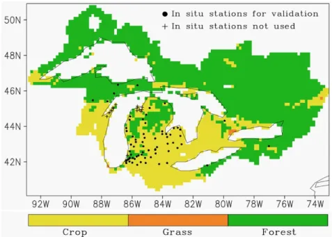
The experiment domain is the Great Lakes basin (Fig. 2.2). The model configurations are similar to those as used in Pietroniro et al. (2007). Seven GRU types are identified for the whole domain: crop, grass, deciduous forest, coniferous forest, mixed forest, water, and impervious. Each GRU class has a different model parameter set. The basin is gridded at 10 arcmins (~ 15 km × 15 km) in the modelling. Each model grid is a mosaic of the seven GRU classes weighted by their cell fractions.

35 cm

410 cm 10 cm

(42)

30

Fig. 2.2 The Great Lakes basin. Note that each grid cell (1/6th of a degree resolution) may consist of a maximum of seven land cover classes (crop, grass, deciduous forest, coniferous forest, mixed forest, water, and impervious). Only the dominant land cover class is displayed for each grid here (the forest cover represents the sum of the deciduous, coniferous, and mixed forest classes). Water and impervious surfaces are not labelled since soil moisture estimates are not considered for them.

2.3 Data assimilation scheme

In a data assimilation system, the observed information is integrated into the model framework by taking into account both the model forecast and observation error characteristics. This allows the model forecast and observation to be optimally merged while without violating the model physical constraints. Many technologies have been developed for land/hydrologic data assimilation (Table A1). In the present study, we use the ensemble Kalman Filter (EnKF) (Evensen, 1994, 2003) to assimilate synthetic satellite soil moisture in the MESH model. The EnKF, which was first introduced by Evensen (1994), uses a Monte Carlo approach to estimate the forecast and observation error statistics. An ensemble of model states is used to approximate the probability density of

(43)

31

the model state. The ensemble spread defines the forecast error variance and the ensemble mean is considered as the best estimate (Gaussian assumption). Thus, the error covariance equation (as used in the Kalman filer or the extended Kalman filter) for the evolution of the model forecast error information can be replaced by integrating the ensemble of model states forward in time, expressed as

, , , , (2.2)

where M denotes the forecast model operator, _, represents a posterior (analysis) model state at measurement time t-1. _, is a priori (forecast) model state at measurement time t.

, denotes the uncertainties in the model (perturbations to the forcing data or deficiencies

in model parameters/physics). The subscript j is the ensemble member index, counting from 1 to the size of the ensemble N. The observation is perturbed to generate an ensemble of perturbed observations with the ensemble mean equal to the actual observation and the spreading of the ensemble as the observation error variance, i.e.,

, , (2.3)

1

1 , , (2.4)

where and _, represent the actual observation and the perturbed observation at time t, respectively. , and denote the observation error perturbation and the observation error

covariance, respectively. The superscript T denotes the vector transpose. At measurement time t, each of the model forecast state ensemble members _, is updated to _, according to the Kalman analysis equation, given by

(44)

32

where is the measurement operator. denotes the forecast error covariance. In the EnKF, is only implicitly needed through

1 1 , 1 , , 1 , (2.6) 1 1 , 1 , , 1 , (2.7)

Ultimately, through conducting in turn the forecast step (equation 2.2) and the update step (equation 2.5), the observational information is sequentially accumulated into the model state. Throughout this thesis, only the one-dimensional version of the Ensemble Kalman filter (1D-EnKF) is used where the horizontal correlations between the model grids are neglected and an observation influences only the model state at the observation location. The model state vector x, which has a dimension of 21 and is independent for each grid, is comprised of the volumetric liquid water content from the seven GRUs for the three soil layers. The observation is the perturbed satellite retrievals of surface soil moisture, and the corresponding model prediction denotes the volumetric liquid water content (a weighted sum of GRUs within the grid) in the model surface layer.

2.4 Experiment setup and results

The synthetic experiment is designed as follows. First, the standalone MESH is integrated for one year period (1 January to 31 December) using the meteorological forcings derived from the Global Environmental Multiscale (GEM) model (Mailhot et al., 2006) forecasts of year 2005. Each GRU class has its own model parameter set, which was based upon a

(45)

33

global calibration with streamflow observations (Haghnegahdar et al., 2014). The model integration is spun up by a repeated integration with the GEM forcings of year 2004. The simulated soil moisture serves as the reference solution (“truth”). The synthetic satellite soil moisture retrievals are generated, independently for each model grid, by applying random noise (the error standard deviation is set to 0.08 m3_/m3_{) to the true surface soil} moisture sequence. Next, an open loop model simulation (without data assimilation), which intentionally deviates from the true integration, is performed. To this end, the MESH model is integrated for a one-year period again but with the GEM forcings of year 2006 and using a different set of model parameters, which are generated by adding random noise with a standard deviation of 30% (of magnitude) to the model parameters used in the true integration. Finally, the synthetic soil moisture retrievals are assimilated into the open-loop integration, under different conditions, to examine the capability of the assimilation system to recover the true soil moisture. The assimilation experiments are listed in Table 2.1. More details on the experiments will be provided in the remainder of this section.

Table 2.1 List of synthetic experiments

Key Description A Control experiment; Ensemble size N = 12; Assimilation interval is 24 hours

B1 Same as A, but with N = 6 B2 Same as A, but with N = 50 B3 Same as A, but with N = 100

C1 Same as A, but with assimilation interval of 12 hours C2 Same as A, but with assimilation interval of 72 hours D1 Same as A, except for a higher retrieval skill

D2 Same as A, except for a lower retrieval skill

(46)

34 A. Control experiment

Experiment A is a control case. We use the 1D-EnKF with 12 ensemble members. To represent random errors in the forcing inputs, the cross-correlated forcing perturbation fields are generated (Table 2.2) following Reichle et al. (2007). Additionally, to account for the model uncertainties due to imperfect model parameters, temporally correlated error perturbations are added to the simulated volumetric liquid water content. Currently, the 0.001 m3_/m3_{, 0.0005 m}3_/m3_{, and 0.00005 m}3_/m3 _{error standard deviations are applied to the} three soil layers, respectively (Table 2.2). The model error parameters are specified largely based upon order-of-magnitude considerations and are not on-line (adaptively) tuned in our assimilation. Smaller error parameters are applied to deeper soil layers to avoid the bias between the ensemble mean (without assimilation) and the unperturbed open-loop integration. The model error correlation time is set to 1 day. A true observation error standard deviation of 0.08 m3_/m3 _{is used for the synthetic retrievals (Recall that the} synthetic retrievals are generated by adding white noise with standard deviation of 0.08 m3_/m3_{to the true surface soil moisture). The assimilation is performed at 24-hr intervals} (i.e., we assume the observing frequency of once daily). The satellite retrieval-model discrepancies in climatological mean and scale are not present and thus not considered in our twin experiment.

(47)

35

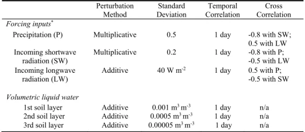
Table 2.2 Error parameters for the selected forcing inputs and model variables Perturbation

Method Deviation Standard Correlation Temporal Correlation Cross Forcing inputs*

Precipitation (P) Multiplicative 0.5 1 day -0.8 with SW;

0.5 with LW Incoming shortwave

radiation (SW) Multiplicative 0.2 1 day -0.8 with P; -0.5 with LW Incoming longwave

radiation (LW) Additive 40 W m

-2 _{1 day} _{0.5 with P;}

-0.5 with SW Volumetric liquid water

1st soil layer Additive 0.001 m3_m-3 _{1 day} _n/a

2nd soil layer Additive 0.0005 m3_m-3 _{1 day} _n/a

3rd soil layer Additive 0.00005 m3_m-3 _{1 day} _n/a

* _{Error parameters for the selected forcing inputs are adapted from Reichle et al. (2007).}

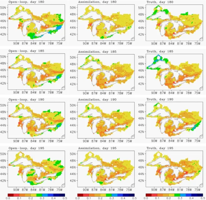
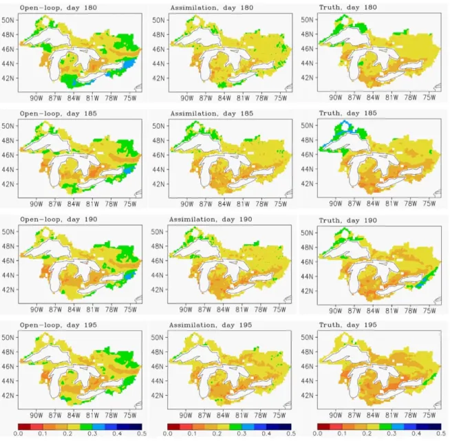
Figure 2.3 shows the open-loop (without assimilation) and the assimilation surface (0-10 cm) soil moisture estimates across the study domain, in comparison with the ‘true’ state. The assimilation estimates show, relative to open loop, better overall agreement with the true fields in terms of the distribution and magnitude of soil moisture across the study domain. This demonstrates that the EnKF scheme installed for the MESH model is effective to improve the model surface soil moisture estimates. The counterpart of Fig. 2.3 for root-zone (0-35 cm) soil moisture is provided in Fig. 2.4. The root-zone soil moisture estimates are also improved through the assimilation of the surface soil moisture retrievals. The successful updating of root-zone soil moisture indicates that through data assimilation, the near-surface soil moisture information, which can be acquired by satellite microwave remote sensing, can spread to deeper soil layers that are not directly measured by satellite sensors. Note that an efficient constraint of satellite retrievals on root-zone soil moisture relies upon the model’s accurate description of water movement in the soil column. In our twin experiment, the model physics is perfect since we used the same model (but with different model parameters) to generate the “true” state and to assimilate soil moisture