HAL Id: hal-02388646
https://hal-enpc.archives-ouvertes.fr/hal-02388646
Submitted on 2 Dec 2019
HAL
is a multi-disciplinary open access
archive for the deposit and dissemination of
sci-entific research documents, whether they are
pub-lished or not. The documents may come from
teaching and research institutions in France or
abroad, or from public or private research centers.
L’archive ouverte pluridisciplinaire
HAL
, est
destinée au dépôt et à la diffusion de documents
scientifiques de niveau recherche, publiés ou non,
émanant des établissements d’enseignement et de
recherche français ou étrangers, des laboratoires
publics ou privés.
variational problems: applications from image
processing to computational mechanics
Jeremy Bleyer
To cite this version:
Jeremy Bleyer. Automating the formulation and resolution of convex variational problems:
applica-tions from image processing to computational mechanics. 2019. �hal-02388646�
variational problems: applications from image processing to
computational mechanics
JEREMY BLEYER,
Laboratoire Navier UMR 8205 (ENPC-IFSTTAR-CNRS), Université Paris-Est, France Convex variational problems arise in many fields ranging from image processing to fluid and solid mechan-ics communities. Interesting applications usually involve non-smooth terms which require well-designed optimization algorithms for their resolution. The present manuscript presents the Python package called fenics_optimbuilt on top of the FEniCS finite element software which enables to automate the formulation and resolution of various convex variational problems. Formulating such a problem relies on FEniCS domain-specific language and the representation of convex functions, in particular non-smooth ones, in the conic programming framework. The discrete formulation of the corresponding optimization problems hinges on the finite element discretization capabilities offered by FEniCS while their numerical resolution is carried out by the interior-point solver Mosek. Through various illustrative examples, we show that convex optimization problems can be formulated using only a few lines of code, discretized in a very simple manner and solved extremely efficiently.CCS Concepts: •Mathematics of computing→Convex optimization; •Computing methodologies →Symbolic and algebraic algorithms;
Additional Key Words and Phrases: convex optimization, conic programming, finite element method, FEniCS ACM Reference Format:
Jeremy Bleyer. 2019. Automating the formulation and resolution of convex variational problems: applications from image processing to computational mechanics. 1, 1 (November 2019),31pages.https://doi.org/10.1145/ nnnnnnn.nnnnnnn
1 INTRODUCTION
Convex variational problems represent an important class of mathematical abstractions which can be used to model various physical systems or provide a natural way of formulating interesting problems in different areas of applied mathematics. Moreover, they also often arise as a relaxation of more complicated non-convex problems. Optimality conditions of constrained convex variational problems correspond to variational inequalities which have been the topic of a large amount of work in terms of analysis or practical applications [25,30,45].
In this work, we consider convex variational problems defined on a domainΩ ⊂Rd(d=2,3 for typical applications) with convex constraints of the following kind:
inf
u∈V J(u)
s.t. u∈ K (1)
whereubelongs to a suitable functional spaceV,J is a convex function andKa convex subset
ofV. Some variational inequality problems are formulated naturally in this framework such as
the classical Signorini obstacle problem in whichKencodes the linear inequality constraint that
a membrane displacement cannot interpenetrate a fixed obstacle (see section3.1). An important
Author’s address: Jeremy Bleyer, [email protected], Laboratoire Navier UMR 8205 (ENPC-IFSTTAR-CNRS), Université Paris-Est, 6-8 av Blaise Pascal, Cité Descartes, Champs-sur-Marne, France, 77455.
© 2019 Association for Computing Machinery.
This is the author’s version of the work. It is posted here for your personal use. Not for redistribution. The definitive Version of Record was published in ,https://doi.org/10.1145/nnnnnnn.nnnnnnn.
class of situations concerns the case whereJ can be decomposed as the sum of a smooth and a non-smooth term. Such a situation arises in many variational models of image processing problems such as image denoising, inpainting, deconvolution, decomposition, etc. In some cases, such as limit analysis problems in mechanics for instance, smooth terms inJare absent so that numerical resolution of (1) becomes very challenging [27,45]. Important problems in applied mathematics such as optimal control [36] or optimal transportation [9,41,42,46] can also be formulated, in some circumstances, as convex variational problems. This is also the case for some classes of topology optimization problems [10], which can also be extended to non-convex problems involving integer optimization variables [28,48]. Finally, robust optimization in which optimization is performed while taking into account uncertainty in the input data of (1) has been developed in the last decade [7,8]. It leads, in some cases, to tractable optimization problems fitting the same framework, possibly with more complex constraints.
The main goal of this paper is to present a numerical toolbox for automating the formulation and the resolution of discrete approximations of (1) using the finite-element method. The large variety of areas in which such problems arise makes us believe that there is a need for a versatile tool which will aim at satisfying three important features:
• straightforward formulation of the problem, mimicking in particular the expression of the
continuous functional;
• automated finite-element discretization, supporting not only standard Lagrange finite
ele-ments but also DG formulations andH(div)/H(curl)elements;
• efficient solution procedure for all kinds of convex functionals, in particular non-smooth
ones.
In our proposal, the first two points will rely extensively on the versatility and computational efficiency of the FEniCS open-source finite element library [2,32]. FEniCS is now an established
collection of components including the DOLFIN C++/Python Interface [34,35], the Unified Form
Language [1,3], the FEniCS Form Compiler [31,33], etc. Using the high-level DOLFIN interface, the user is able to write short pieces of code for automating the resolution of PDEs in an efficient
manner. For all these reasons, we decided to develop a Python package calledfenics_optimas an
add-on to the FEniCS library. We will also make use of Object Oriented Programming possibilities
offered by Python for defining easily our problems (see 4.4). Our proposal can therefore be
considered to be close to high-level optimisation libraries based ondisciplined convex programming
such as CVX1for instance. However, here we really concentrate on the integration within an
efficient finite-element library offering symbolic computation capabilities. As mentioned later, in-tegration with other high-level optimisation libraries will be an interesting development perspective. Concerning the last point on solution procedure, we will here rely on the state-of-the art
conic programming solver named Mosek [38], which implements extremely efficient primal-dual
interior-point algorithms [4]. Let us mention first that there is no ideal choice concerning solution algorithms which mainly depends on the desired level of accuracy, the size of the considered problem, the sparsity of the underlying linear operators, the type of convex functionals involved, etc. In particular, in the image processing community, first-order proximal algorithms are widely used since they work well in practice for large scale problems discretized on uniform grids [41]. Moreover, high accuracy on the computed solution is usually not required since one aims mostly at achieving some decrease of the cost function but not necessarily an accurate computation of the optimal point. In contrast, interior-point methods can achieve a desired accuracy on the solution in polynomial time and, in practice, in quasi-linear time since the number of final iterations is 1http://cvxr.com/cvx/
often observed to be nearly independent on the problem size. However, as a second-order method, each iteration is costly since it requires to solve a Newton-like system. Iterative solvers are also difficult to use in this context due to the strong increase of the Newton system conditioning when approaching the solution. As result, such solvers usually rely on direct solvers for factorizing the resulting Newton system, therefore requiring important memory usage. Nevertheless, interior-point solvers are extremely robust and quite efficient even compared to first order methods in some cases. For these reasons, the present paper will not focus on comparing different solution procedures and we will use only the Mosek solver but including first-order algorithms in the
fenics_optimpackage will be an interesting perspective for future work. Providing interfaces to other interior-point solvers, especially open-source ones (CVXOPT, ECOS, Sedumi, etc.), is also planned for future releases.
The manuscript is organized as follows: section2introduces the conic programming framework
and the concept of conic representable functions. The formulation and discretization of convex
variational problems is discussed in section3by means of a simple example. Section4discusses
further aspects by considering a more advanced example. Finally,5provides a gallery of illustrative examples along with their formulation and some numerical results.
The fenics_optim package can be downloaded from https://gitlab.enpc.fr/navier-fenics/ fenics-optim. It contains test files as well as demo files corresponding to the examples discussed in the present paper.
2 CONIC PROGRAMMING FRAMEWORK
2.1 Conic programming in Mosek
The Mosek solver is dedicated to solving problems entering theconic programming framework
which can be written as:
min x c Tx s.t. bl ≤Ax≤bu x∈ K (2)
where vectorcdefines a linear objective functional, matrixA and vectorsbu,bl define linear
inequality (or equality ifbu =bl) constraints and whereK=K1× K2×. . .× Kpis a product of conesKi ⊂Rdi so thatx∈ K ⇔xi ∈ Ki∀i =1, . . . ,pwherex=(x1,x2, . . . ,xp). These cones can be of different kinds:
• Ki =Rdi i.e. no constraint onxi
• Ki =(R+)di is the positive orthant i.e.xi ≥0
• Ki =Qdi the quadratic Lorentz cone defined as:
Qdi ={z∈Rdi s.t.z=(z
0,z)¯ andz0 ≥ ∥z∥¯ 2} (3)
• Ki =Qdr
i the rotated quadratic Lorentz cone defined as:
Qdr
i ={z∈R
di s.t.z=(z
0,z1,z)¯ and 2z0z1≥ ∥¯z∥22} (4)
• Ki =Sdi is the vectorial representation of the cone of semi-definite positive matricesS+ni of dimensionni ifdi =ni(ni +1)/2 i.e.
Sdi ={vec(M)s.t.M∈S+n
i} (5)
whereS+ni ={M ∈R
ni×ni s.t.M =MTandM ⪰0}
and in which thevecoperator is the half-vectorization of a symmetric matrix obtained by
arranged in a column-wise manner and off-diagonal elements are multiplied by a√2 factor. For instance, for a 3×3 matrix:
vec(M)=(M1,1, √ 2M1,2, √ 2M1,3,M2,2, √ 2M2,3,M3,3) (6)
Note that this representation is such thatvec(A)Tvec(B)=⟨A,B⟩F where⟨·,·⟩F denotes the Froebenius inner product of two matrices.
IfK contains only cones of the first two kinds, then the resulting optimization problem (2)
belongs to the class of Linear Programming (LP) problems. If, in addition,Kcontains quadratic
conesQdiorQ
r
di, then the problem belongs to the class of Second-Order Cone Programming (SOCP)
problems. Finally, when cones of the typeSdi are present, the problem belongs to the class of
Semi-Definite Programming (SDP) problems. Note that Quadratic Programming (QP) problems consisting of minimizing a quadratic functional under linear constraints can be seen as a particular instance of an SOCP problem as we will later discuss.
There obviously exist dedicated algorithms for some classes of problem (e.g. the simplex method for LP, projected conjugate gradient methods for bound constrained QP, etc.). However, interior-point algorithms prove to be extremely efficient algorithms for all kinds of problems from LP up to difficult problems like SDP. It also turns out that a large variety of convex problems can be reformulated into an equivalent problem of the previously mentioned categories so that interior-point algorithms can be used to solve, in a robust and efficient manner, a large spectrum of convex optimization problems.
2.2 Conic reformulations
Most conic programming solvers other than Mosek (CVXOPT, Sedumi, SDPT3) use a default format similar to (2). Aiming at optimizing a convex problem using a conic programming framework therefore requires a first reformulation step to fit into format (2). In the following examples, we will consider a purely discrete setting in which optimization variables are inRn.
2.2.1 L2-norm constraint.Let us consider the followingL2-norm constraint:
∥x∥2≤1 (7)
This can be readily observed to be the following quadratic cone constraint(1,x) ∈ Qn+1. However, for this constraint to fit the general format of (2), one must introduce an additional scalar variable ysuch that the previous constraint can be equivalently written:
y=1 (8)
∥x∥2 ≤y⇔ (y,x) ∈ Qn+1
2.2.2 L1-norm constraint.Let us consider the followingL1-norm constraint:
∥x∥1=
n
Õ
i=1
|xi| ≤1 (9)
To reformulate this constraint, we introducenscalar auxiliary variablesyi such that:
n
Õ
i=1
yi =1 (10)
|xi| ≤yi ∀i
then each constraint with an absolute value can be written using two linear inequality constraints xi−yi ≤0 and 0≤xi+yi.
2.2.3 Quadratic constraint. Let us consider the case of a quadratic inequality constraint such as: 1
2x
TQx≤b (11)
MatrixQmust necessarily be semi-definite positive for the constraint to be convex. In this case, introducing the Cholesky factorCofQsuch thatQ=CTC, one has:
1 2x T Qx= 1 2∥Cx∥ 2 2 ≤b (12)
Introducing an auxiliary variabley, the previous constraint can be equivalently reformulated as:
Cx−y=0 (13)
∥y∥22 ≤2b Finally adding two others scalar variablesz0andz1, we have:
Cx−y=0 (14)
z0=b z1=1
∥y∥22 ≤2z0z1
where the last constraint is also the rotated quadratic cone constraint(z0,z1,y) ∈ Qnr+2
2.2.4 Minimizing aL2-norm.Let us now consider the problem of minimizing theL2-norm ofBx
under some affine constraints:
min
x ∥Bx∥2
s.t. Ax=b (15)
As such this problem does not fit (2) since the objective function is non-linear. In order to circumvent this, one needs to consider the epigraph ofF(x)=∥Bx∥2defined as epiF ={(t,x)s.t.F(x) ≤t}. MinimizingFis then equivalent to minimizingtunder the constraint that(t,x) ∈epiF. For the present case, we therefore have:
min
x,t t Ax=b ∥Bx∥2≤t
(16)
Introducing an additional variableywe have: min x,y,t t Ax=b Bx−y=0 ∥y∥2 ≤t (17)
where the last constraint is again a quadratic Lorentz cone constraint. Problem (15) is now a linear problem of the augmented optimization variables(x,y,t)under linear and conic constraints. 2.3 Conic representable sets and functions
As previously mentioned, minimizing a convex functionF(x)can be turned into a linear problem with a convex non-linear constraint involving the epigraph ofF. We will thus consider the class of
conic representable functionsas the class of convex functions which can be expressed as follows: F(x)=min y c T xx+cTyy s.t. bl ≤Ax+By≤bu y∈ K (18)
in whichKis again a product of cones of the kinds detailed in section2.1. For instance, consider the case of theL1-norm, we have:
∥x∥1=min y∈Rn e Ty s.t. 0≤x+y x−y≤0 (19)
wheree=(1, . . . ,1)whereas for theL2-norm we have:
∥x∥2= min
y∈Rn+1 y0
s.t. x−¯y=0 y∈ Qn+1
(20)
wherey=(y0,y1, . . . ,yn)and¯y=(y1, . . . ,yn). In this example, it can be seen that the representa-tion (18) is not necessarily optimal in terms of number of additional variables, one could perfectly eliminate theyvariable. However, in most practical cases, functions like theL2-norm will quite often be composed with some linear operator (gradient, interpolation, etc.) so that introducing such additional variables will be necessary to fit format (2).
Obviously, ifFis the indicator function of a convex set, then we have a similar notion ofconic representable setsfor which only the constraints in (18) are relevant.
3 VARIATIONAL PROBLEMS AND THEIR DISCRETE VERSION
3.1 A first illustrative example
Before describing the framework of variational formulation and discretization, let us first intro-duce a classical example of variational inequality, namely the obstacle problem. LetΩbe a bounded domain ofR2andu ∈V =H01(Ω), f ∈H
−1(Ω)andд ∈H1(Ω) ∩C0such thaty ≤0 on∂Ω. The obstacle problem consists in solving:
inf u∈V ∫ Ω 1 2∥∇u∥ 2 2dx− ∫ Ωf udx s.t. u∈ K (21) where K = {v ∈ H1
0(Ω)s.t.v ≥ дonΩ}. Physically, this problem corresponds to that of a
membrane described by an out-of-plane deflectionuand loaded by a vertical loadf which may
potentially enter in contact with a rigid obstacle located on the surfacez=−д(x,y). 3.2 Discretization
Let us now consider some finite element discretization ofΩusing a meshThofNetriangular cells. For the displacement fieldu, we consider a Lagrange piecewise linear interpolation represented by the discrete functional spaceVh = {v ∈ C0(Ω)s.t.v|T ∈ P1(T) ∀T ∈ Th}of dimensionN.
Interpolating the obstacle positionyon the same spaceVh, a discrete approximationKh ofK
consists in a pointwise inequality on the vectorsv,g∈RN of degrees of freedom ofvh,дh ∈Vh:
the first integral in (21), the discrete obstacle problem is now: min u∈RN M Õ д=1 ωд1 2∥Bдu∥ 2 2−fTu s.t. u≥g (22)
In (22),Bдu∈R2denotes the discrete gradient evaluated at the current quadrature pointдandωд
is the associated quadrature weight. Note that sinceuhis linear, its gradient is piecewise-constant
so that only one point per triangleT withωд=|T|is sufficient for exact evaluation of the integral
(M=Nein this case). Finally,fis the assembled finite-element vector corresponding to the linear
formL(u)=∫Ωf udx.
The quadratic term in the objective function is now rewritten following section2.2as follows:
min u∈RN M Õ д=1 ωдyд,0−fTu s.t. u≥g yд,1=1 Bдu− y д,2 yд,3 =0 ∀д=1, . . . ,M (yд,0,yд,1,yд,2,yд,3) ∈ Qr4 (23)
Collecting the 4M auxiliary variables yд = (yд,0,yд,1,yд,2,yд,3) into a global vectorby =
(y1, . . .yM) ∈R4M, the previous problem can be rewritten as:
min u∈RN, by∈R 4M c T by−f T u s.t. u≥g Auu+Ayby=b by∈ Q r 4× · · · × Q4r (24) where c = (ω1,0,0,0,ω2,0. . . ,ωM,0,0,0), Au = 0 B1 0 B2 .. . 0 BM , Ay = −I . .. −I with I = 0 1 0 0 0 0 1 0 0 0 0 1
andb=(1,0,0,1,0. . . ,1,0,0). This last formulation enables to see that problem (22) indeed fits into the general conic programming framework (2) but in a specific fashion since it possesses a block-wise structure induced by the quadrature rule. Indeed, each 4-dimensional
block of auxiliary variablesyдis decoupled from each other and is linked to the main unknown
variableuthrough the evaluation of the discrete gradient at each pointд. The conic reformulation performed in (22) is in fact the same for all quadrature points.
This observation motivates us to rewrite the initial continuous problem as: inf u∈V ∫ ΩF(∇u)dx− ∫ Ωf udx s.t. u∈ K (25)
withF(x)= 1
2∥x∥ 2
2which is conic representable as follows2: F(x)=min y∈R4 y0 s.t. y1=1 x− y2 y3 =0 y∈ Q4r (26)
Introducing now the previously mentioned discretization and the quadrature formula, we aim at solving: min u∈RN M Õ д=1 ωдF(Bдu) −fTu s.t. u≥g (27) which will be equivalent to (22) when injecting (26) into (27) since, for allMevaluations ofF, a 4-dimensional auxiliary vectoryдwill be introduced as an additional minimization variable.
As a consequence, thefenics_optimpackage has been particularly designed for a sub-class of
problems of type (1) in whichJ(u)=∫Ωj(u)dx for which integration will be handled by the FEniCS machinery and in which the user must specify the local conic representation ofj.
3.3 FEniCS formulation
In the following, we present the main part of afenics_optimscript. More details on how an
optimization problem is defined are discussed inA. In particular, it is possible to writemanually
the discretized version of the obstacle problem based on (24) (seeA.2). However,fenics_optim
also provides a more user-friendly way of modelling such problems which is based on (25) and (26) and will now be presented.
First, a simple unit square mesh andP1Lagrange function spaceVis defined using basic FEniCS
commands. Homogeneous Dirichlet boundary conditions are also defined in variablebc. Finally,
obstacleis the interpolant onV of
д(x,y)=д0+asin(2πk1x)cos(2πk1y)sin(2πk2x)cos(2πk2y)
In the following simulations, we tookд0=−0.1,a=0.01,k1=2 andk2=8. The loading is also
assumed to be uniform and given byf =−5. The main part of the script starts by instantiating
aMosekProblemobject and adding a first optimization variableuliving in the function spaceV,
subject to Dirichlet boundary conditionsbc. Theadd_varmethod also enables to define a lower
bound (resp. an upper bound) on an optimization variable by specifying a value for thelx(resp.
ux) keyword. For the present case, we uselx=obstaclefor enforcingu≥g.
1 prob = MosekProblem("Obstacle problem") 2 u = prob.add_var(V, bc=bc, lx=obstacle) 3
4 prob.add_obj_func(-dot(load,u)*dx)
where we also added the linear part of the objective function through theadd_obj_funcmethod.
The next step consists in defining the quadratic part of the objective function. For this purpose,
we define a class inheriting from the baseMeshConvexFunctionclass which must be instantiated
by specifying on which previously defined optimization variable3this function will act (here the
only possible variable isu). Moreover, we also specify the degree of the quadrature necessary
2Note that it would have been possible to work directly with function e
F(u):=12∥ ∇u∥2
2which is also conic-representable 3see the notion of block-variables discussed inA.
for integrating the function (one-point quadrature used by default but written explicitly in the
code snippet below). We must also define theconic_reprmethod which will encode the conic
representation (26). We add a local optimization variableYof dimension 4 which will belong to the coneRQuad(4)representingQ4r. Equality constraints are then added using theadd_eq_constraint
by specifying, as in (18), a block matrix
A B
and a right-hand sideb(=0 by default). Note that both equality constraints could also have been written in a single one of row dimension 3. Finally, the local linear objective(cx,cy)vector is defined using theset_linear_termmethod.
1 class QuadraticTerm(MeshConvexFunction): 2 def conic_repr(self, X):
3 Y = self.add_var(4, cone=RQuad(4))
4 self.add_eq_constraint([None, Y[1]], b=1)
5 self.add_eq_constraint([X, -as_vector([Y[2], Y[3]])]) 6 self.set_linear_term([None, Y[0]])
7
8 F = QuadraticTerm(u, degree=0) 9 F.set_term(grad(u))
10 prob.add_convex_term(F)
Note that constraints and linear objectives are all defined in a block-wise manner, these blocks consisting of, first, the main variable which has been specified at instantiation (uin this case), then the additional local variables (Yhere). Besides, these blocks are represented in terms of their action on the block variables using UFL expressions.
Theset_termmethod enables to evaluateF for the gradient ofuusing the UFLgradoperator. This function is then added to the global optimization problem. Finally, optimization (minimization
by default) is performed by calling theoptimizemethod of theMosekProblemobject:
1 prob.optimize()
For validation and performance comparison, the obstacle problem has been solved for
vari-ous mesh sizes using thefenics_optimtoolbox as well as using PETSc’s TAO quadratic
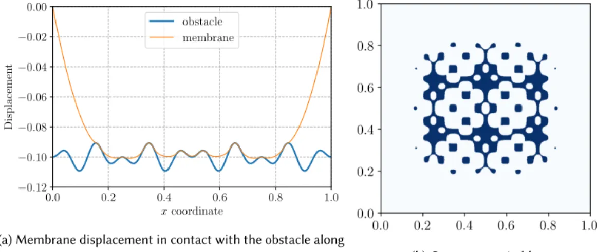
bound-constrained solver [5,39] which is particularly well suited for this kind of problems. We used the Trust Region Newton Method (TRON) and an ILU-preconditioned conjugate gradient solver for the inner iterations. Results in terms of optimal objective function value, total optimization time and number of iterations have been reported for both methods in table1. Note that default convergence tolerances have been used in both cases and that total optimization time includes the presolve step of Mosek which can efficiently eliminate redundant linear constraints for instance. It can be observed that both approach yield close results in terms of optimal objective values and that TAO’s solver is more efficient than Mosek in terms of optimization time as expected, mainly because of the small number of iterations needed to reach convergence but also because no additional variables are introduced when using TAO. However, Mosek surprisingly becomes quite competitive for large-scale problems because of its number of iterations scaling quite weakly with the problem size, contrary to the TRON algorithm. Membrane displacement along the liney=0.5 and contact area forh=1/400 have been represented in Figure1.
4 A MORE ADVANCED EXAMPLE
Let us now consider the following problem: inf u∈V ∫ Ω∥∇u∥2dx s.t. ∫Ωf udx=1 (28)
Mesh size Interior point (Mosek) TRON algorithm (TAO)
Objective Opt. time iter. Objective Opt. time iter.
h=1/25 -0.265081 0.13 s 14 -0.265082 0.09 s 5
h=1/50 -0.264932 0.56 s 15 -0.264932 0.22 s 6
h=1/100 -0.264883 2.27 s 16 -0.264884 1.04 s 10
h=1/200 -0.264867 10.04 s 19 -0.264871 6.03 s 14
h=1/400 -0.264864 48.95 s 20 -0.264868 47.79 s 22
Table 1. Comparison between thefenics_optimimplementation of the obstacle problem relying on the interior point Mosek solver and TAO’s bound-constrained TRON solver.
0.0 0.2 0.4 0.6 0.8 1.0 xcoordinate −0.12 −0.10 −0.08 −0.06 −0.04 −0.02 0.00 Displacemen t obstacle membrane
(a) Membrane displacement in contact with the obstacle along
y=0.5 (b) Contact area in blue Fig. 1. Results of the obstacle problem forh=1/400
This problem is known to be related to antiplane limit analysis problems in mechanics as well as to the Cheeger problem and the eigenvalue fo the 1-Laplacian whenf =1 [16,17,20]. In this particular case, the solution of (28) can indeed be shown to be proportional to the characteristic
function of a subsetCΩ⊆Ωknown as the Cheeger set ofΩwhich is the solution of:
CΩ:= argmin
ω⊆Ω
|∂ω|
|ω| (29)
that is the subset minimizing the ratio of perimeter over area, the associated optimal value of this ratiocΩbeing known as theCheeger constant.
This problem is not strictly convex and is particularly difficult to solve using standard algorithms due to the highly non-smooth objective term. Again, introducing aPkLagrange discretization for
u, we aim at solving the following discrete problem: min u∈RN M Õ д=1 ωдF(Bдu) s.t. fTu=1 (30)
whereF(x) = ∥x∥2 with its conic representation being given by (20). Similarly to the obstacle
objective function evaluation. ForPkwithk ≥2, the quadrature is always inexact and Gaussian
quadrature is not necessarily optimal. For the particular casek = 2, one can choose a vertex
quadrature scheme on the simplex triangle to ensure that the discrete integral is approximated by excess: ∫ T ∥r(x,y )∥dx≲ |T| 3 3 Õ i=1 ∥r(xi,yi)∥ (31)
where(xi,yi)denote the simplex vertices. The choice of the quadrature scheme can also be made
when defining the correspondingMeshConvexFunction:
1 class L2Norm(MeshConvexFunction):
2 """ Defines the L2-norm function ||x||_2 """ 3 def conic_repr(self, X):
4 d = self.dim_x
5 Y = self.add_var(d+1, cone=Quad(d+1))
6 Ybar = as_vector([Y[i] for i in range(1, d+1)]) 7 self.add_eq_constraint([X, -Ybar])
8 self.set_linear_term([None, Y[0]]) 9
10 prob = MosekProblem("Cheeger problem") 11 u = prob.add_var(V, bc=bc) 12 13 if degree == 1: 14 F = L2Norm(u) 15 elif degree == 2: 16 F = L2Norm(u, "vertex") 17 else:
18 F = L2Norm(u, degree = degree) 19 F.set_term(grad(u))
20 prob.add_convex_term(F)
In the previous code,degreedenotes the polynomial degreek of function spaceV. Ifk =1,
the default one-point quadrature rule is used, ifk = 2 the above-mentionedvertexscheme is
used, otherwise a default Gaussian quadrature rule for polynomials of degreek is used.Quad(d+1)
corresponds to the quadratic Lorentz coneQd+1of dimensiond+1 whered=self.dim_xis the dimension of theXvariable.
In the Cheeger problem, a normalization constraint must also be added. This can again be done by adding a convex term including only the corresponding constraint or it can also be added
directly to theMosekProbleminstance by defining the function space for the Lagrange multiplier
corresponding to the constraint (here it is scalar so we use a"Real"function space) and passing the corresponding constraint in its weak form as follows:
1 f = Constant(1.)
2 R = FunctionSpace(mesh, "Real", 0) 3 def constraint(l):
4 return [l*f*u*dx]
5 prob.add_eq_constraint(R, A=constraint, b=1)
4.1 Discontinuous Galerkin discretization
Problem (28) can be discretized using standard Lagrange finite elements but also using Discon-tinous Galerkin discretization, in this case the gradientL2-norm objective term is completed by
absolute values of the jumps ofu: min u∈V ∫ Ω ∥∇u∥2dx+ ∫ Γ |[[u]]|dS+ ∫ ΓD |u|dS s.t. ∫Ωf udx=1 (32)
whereΓdenotes the set of internal edges,ΓDthe Dirichlet boundary part and[[u]]=u+−u−is the jump acrossΓ.
The discretized version using discontinuousPdkLagrange finite elements reads as:
min u∈RN M Õ д=1 ωдF(Bдu)+ Me Õ дe=1 ωдeG(Jдeu)+ Md Õ дd=1 ωдdG(Tдdu) s.t. fTu=1 (33)
whereG(x)=|x|,дe(resp.дd) denotes a current quadrature point on the internal (resp. Dirichlet) facets,Me (resp.Md) denoting the total number of such points andωдe (resp.ωдd) the associated quadrature weights. Finally,Jдeudenotes the evaluation of[[u]]at the quadrature pointдeandTдdu the evaluation ofuatдd.
Similarly to the previously introducedMeshConvexFunction, we define aFacetConvexFunction
corresponding to the conic representable convex functionG(x):
1 class AbsValue(FacetConvexFunction): 2 def conic_repr(self, X):
3 Y = self.add_var()
4 self.add_ineq_constraint(A=[X, -Y], bu=0) 5 self.add_ineq_constraint(A=[-X, -Y], bu=0) 6 self.set_linear_term([None, Y])
When instantiating such aFacetConvexFunction, integration will (by default) be performed
both on internal edges (in FEniCS the corresponding integration measure symbol isdS) and on
external edges (FEniCS symbol beingds). If the Dirichlet boundary does not cover the entire
boundary, then thedsmeasure can be restricted to the corresponding part. Again, the optimization variable on which acts the function must be specified and the desired quadrature rule can also be
passed as an argument when instantiating the function. Theset_termmethod can now take a
list of UFL expression associated to the different integration measures. In the present case,Gis evaluated for[[u]]ondSand foruonds:
1 G = AbsValue(u)
2 G.set_term([jump(u), u]) 3 prob.add_convex_term(G)
By default, facet integrals are evaluated using thevertexscheme. 4.2 Numerical example
We consider the problem of finding the Cheeger set of the unit squareΩ =[0; 1]2. The exact
solution of this problem is known to be the unit square rounded by circles of radiusρ= 1
2+√π in its four corners, the associated Cheeger constant beingcΩ=1/ρ[40,44]. Results of the optimal fieldufor various discretization schemes have been represented on Figure2. For all the retained discretization choices, the obtained Cheeger constant estimates are necessarily upper bounds to the
exact one, in particular because of the choice ofvertexquadrature schemes ensuring upper bound
of the Cheeger set, except for the DG-0 scheme which is too stiff and produces straight edges in the corners, following the structured mesh edges.
4.3 AH(div)-conforming discretization for the dual problem
It can be easily shown through Fenchel-Rockafellar duality that problem (28) is equivalent to the following dual problem (see [17] for instance):
sup λ∈R,σ∈W λ s.t. λf =divσ inΩ ∥σ∥2≤1 (34)
A natural discretization strategy for such a problem is to useH(div)-conforming elements such as the Raviart-Thomas element. Here, we will use the lowest Raviart-Thomas element, notedRT1by the FEniCS definition [32]. For thefenics_optimimplementation, two minimization variables are defined:λbelonging to a scalar"Real"function space andσ ∈RT1. Since forσ ∈RT1, divσ ∈P0, we write the constraint equation usingP0Lagrange multipliers:
1 N = 50
2 mesh = UnitSquareMesh(N, N, "crossed") 3
4 VRT = FunctionSpace(mesh, "RT", 1) 5 R = FunctionSpace(mesh, "Real", 0) 6 VDG0 = FunctionSpace(mesh, "DG", 0) 7
8 prob = MosekProblem("Cheeger dual") 9 lamb, sig = prob.add_var([R, VRT]) 10
11 f = Constant(1.) 12 def constraint(u):
13 return [lamb*f*u*dx, -u*div(sig)*dx]
14 prob.add_eq_constraint(VDG0, A=constraint, name="u")
Finally, sinceσ ∈ P1on a triangle, if the constraint∥σ∥2is satisfied at the three vertices, it
is satisfied everywhere by convexity. We here define aMeshConvexFunctionrepresenting the
characteristic function of aL2-ball constraint and select the"vertex"quadrature scheme so that the constraint will be indeed satisfied at the three vertices. Finally, the objective function is defined
through theadd_obj_funcmethod of the problem instance:
1 class L2Ball(MeshConvexFunction):
2 """ Defines the L2-ball constraint ||x||_2 <= 1 """ 3 def conic_repr(self, X):
4 d = self.dim_x
5 Y = self.add_var(d+1, cone=Quad(d+1))
6 Ybar = as_vector([Y[i] for i in range(1, d+1)]) 7 self.add_eq_constraint([X, -Ybar]) 8 self.add_eq_constraint([None, Y[0]], b=1) 9 10 F = L2Ball(sig, "vertex") 11 F.set_term(sig) 12 prob.add_convex_term(F) 13 14 prob.add_obj_func([1, None])
(a) 25×25 mesh
(b) CG-1 (c) CG-2
(d) DG-0 (e) DG-1
Fig. 2. Results of the Cheeger problem for various discretizations on the unit square: continuous Galerkin (CG) and discontinuous Galerkin (DG) of degreesk=0,1or2.
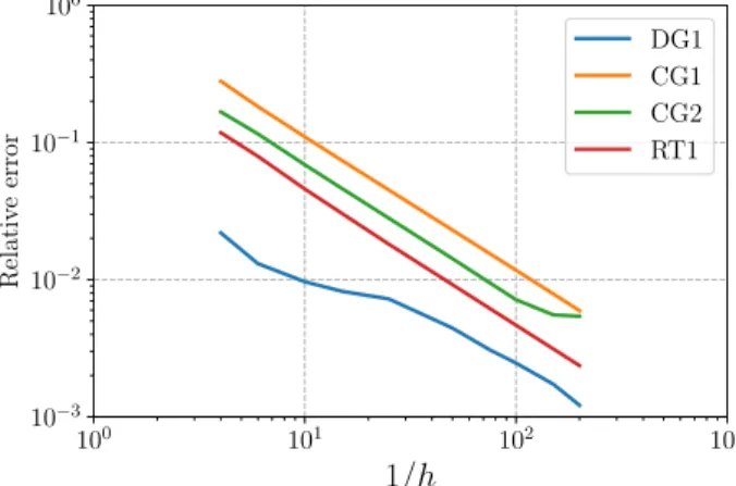
100 101 102 103 1/h 10−3 10−2 10−1 100 Relativ e error DG1 CG1 CG2 RT1
Fig. 3. Convergence results on the Cheeger problem
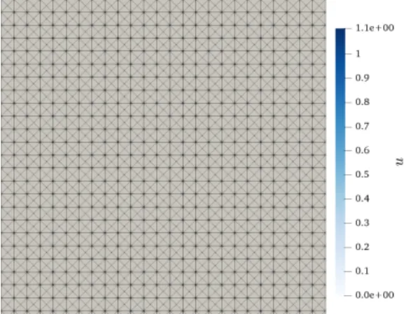
Fig. 4. Optimalufield from the RT discretization
With the above-mentioned discretization and quadrature choice, it can easily be shown that the discrete version of (34) will produce a lower bound of the exact Cheeger constant. For instance, for a 25×25 mesh, we obtained:
cRT1
Ω ≈3.704≤cΩ≈3.772≤cDGΩ 1≈3.800 (35) Convergence results of the numerical Cheeger constant estimatecΩ,hobtained with the previous
CG/DG discretizations as well as with the present RT discretization have been reported in Figure
3. The relative error is computed asϵ(cΩ,h/cΩ−1)whereϵ =−1 for the RT discretization and
ϵ =1 otherwise. We observe in particular that the DG1 scheme is the most accurate and that all
schemes have the same convergence rate inO(h). Finally, primal-dual solvers such as Mosek also provide access to the optimal values of constraint Lagrange multipliers. The Lagrange multiplier associated with the constraintλf =divσcan be interpreted as the fieldufrom the primal problem. This Lagrange multiplier, which belongs to a DG0 space, has been represented in Figure4. 4.4 A library of convex representable functions
In thefenics_optimlibrary, instead of defining each time the conic representation of usual
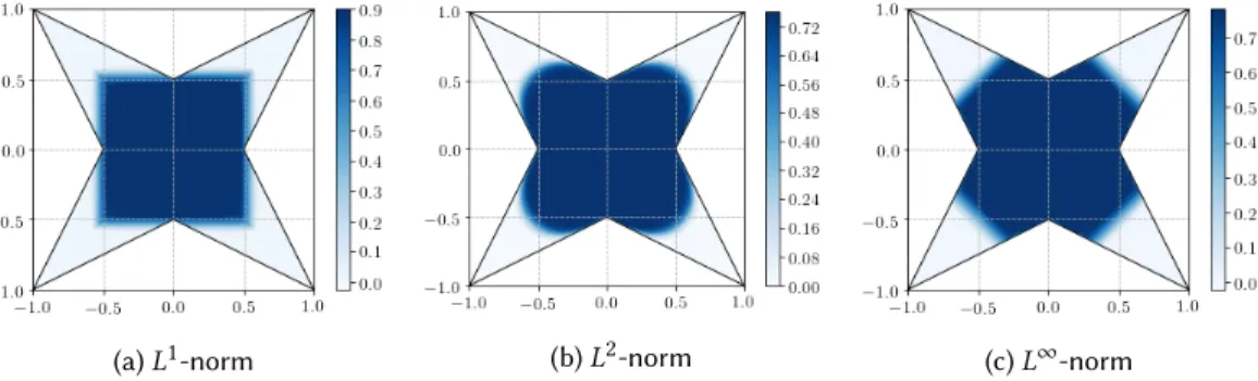
(a)L1-norm (b)L2-norm (c)L∞-norm Fig. 5. Generalized Cheeger sets of a star-shaped domain using different norms
• linear functionsF(x)=cTx
• quadratic functionsF(x)=12(x−x0)TQTQ(x−x0)
• absolute valueF(x)=|x| • L1,L2andL∞norms
• L1,L2andL∞balls characteristic functions
These functions inherit from the composite classConvexFunctionwhich, by default, behaves
like aMeshConvexFunction. To use them asFacetConvexFunction, they can be instantiated asF
= L2Norm.on_facet(u). Using such predefined functions, many problems can be formulated in an extremely simple manner, without even worrying about the conic reformulation. For instance,
we revisited the Cheeger problem on a star-shaped domain but with anisotropic norms [29] such
asL1andL∞instead ofL2in (28)4, the resulting sets are represented on Figure5.
5 A GALLERY OF ILLUSTRATIVE EXAMPLES
We now give a series of examples which illustrate the versatility of thefenics_optimpackage
for formulating and solving problems taken from the fields of solid and fluid mechanics, image processing and applied mathematics. The last two examples involve, in particular, time-dependent problems. Let us again point out that discretization choices or solver strategies using interior-point methods are not necessarily the most optimal ones for each of these problems and that many other approaches which have been proposed in the literature may be much more appropriate. We just aim at illustrating the potential of the package to formulate and solve various problems.
5.1 Limit analysis of thin plates in bending
The first problem consists in finding the ultimate load factor that a thin plate in bending can sustain given a predefined strength criterion and boundary condition. This limit analysis problem has been studied in [12,22]. In the present case, we consider a unit square plate made of a von Mises material of uniform bending strengthmand subjected to a uniformly distributed loadingf. The thin plate limit analysis problem consists in solving the following problem:
inf u∈HB0(Ω) ∫ Ωπ(∇ 2u)dx s.t. ∫ Ωf udx=1 (36)
4Note that in the general case of anLp-norm for the gradient term, the corresponding jump term in (32) is∫
Γ|[[u]] | · ∥n∥pdS wherenis the facet normal and similarly for the Dirichlet boundary term.
where HB0 is the space of bounded Hessian functions [23] with zero trace on∂Ωandπ(M) = 2√m
3 q
M2
11+M222 +M212+M11M22for anyM ∈S+2. One can notice that problem (36) shares some similar structure with the Cheeger problem (28) except that we are now dealing with the Hessian operator and a different norm through functionπ.
Contrary to elastic bending plate problems involving functions withC1-continuity, we deal here with functions in HB which are continuous but may have discontinuities in their normal gradient
∂nu, in particular we can consider again a Lagrange interpolation foruwith jumps of∂nuacross all internal facetsF ∈Γh of unit normaln. Theπ-function being some generalized total variation for∇2u, we have explicitly [13]:
inf u∈HB0(Ω) Õ T∈ Th ∫ Tπ(∇ 2u)dx+Õ F∈Γh ∫ Fπ([[∂nu]]n⊗n)dS s.t. ∫ Ωf udx=1 (37)
where it happens that in factπ([[∂nu]]n⊗n) =|[[∂nu]]|π(n⊗n) =|[[∂nu]]|2√m
3. FollowingB, we have the following formulation of the bending plate problem for aP2interpolation:
1 prob = MosekProblem("Bending plate limit analysis") 2
3 V = FunctionSpace(mesh, "CG", 2)
4 bc = DirichletBC(V, Constant(0.), boundary) 5 u = prob.add_var(V, bc = bc) 6 7 R = FunctionSpace(mesh, "R", 0) 8 def Pext(lamb): 9 return [lamb*dot(load,u)*dx] 10 prob.add_eq_constraint(R, A=Pext, b=1) 11 12 J = as_matrix([[2., 1., 0.], 13 [0, sqrt(3.), 0.], 14 [0, 0, 1]]) 15 def Chi(v): 16 chi = sym(grad(grad(v)))
17 return as_vector([chi[0,0], chi[1,1], 2*chi[0, 1]]) 18 pi_c = L2Norm(u, "vertex", degree=1)
19 pi_c.set_term(m/sqrt(3)*dot(J, Chi(u))) 20 prob.add_convex_term(pi_c) 21 22 pi_h = L1Norm.on_facet(u) 23 pi_h.set_term([jump(grad(u), n)], k=2/sqrt(3)*m) 24 prob.add_convex_term(pi_h) 25 26 prob.optimize()
The reference solution for this problem is known to be 25.02m/f [15], whereas we find 25.05m/f
for a 50×50 structured mesh. The corresponding solutions foruandπ(∇2u)are represented in Figure6.
5.2 Viscoplastic yield stress fluids
Viscoplastic (or yield stress) fluids [6,21] are a particular class of non-Newtonian fluids which, in their most simple form, namely the Bingham model, behave like a purely rigid solid when the
(a) Optimal collapse mechanismu (b) Curvature dissipation densityπ(∇2u)
Fig. 6. Results for the simply supported von Mises square plate
shear stress is below a critical yield stressτ0and flow like a Newtonian fluid when the shear stress is aboveτ0. They appear in many applications ranging from civil engineering, petroleum, cosmetics or food industries. The solution of a steady state viscoplastic fluid flow under Dirichlet boundary conditions and a given external force fieldf can be obtained as the unique solution to the following convex variational principle [26]:
inf u∈H1(Ω; Rd) ∫ Ω(µ∥∇u∥ 2 2+ √ 2τ0∥∇u∥2)dx− ∫ Ωf ·udx s.t. divu =0 inΩ u=дon∂Ω (38)
whereµis the fluid viscosity. Typical solutions of problem (38) involve rigid zones in which∇u =0 and flowing regions where∥∇u∥,0, the locations of which area prioriunknown. Note that when
τ0=0, we recover the classical viscous energy of Stokes flows and optimality conditions of problem (38) reduce to a linear problem. The FE discretization is quite classical, we adopt Taylor-HoodP2/P1
discretization for the velocityuand the pressurepwhich is the Lagrange multiplier of constraint divu =0.
The considered problem is the classical lid-driven unit-square cavity, withf =0,u =0
every-where on∂Ω, except on the top boundaryy=1 whereu =(U,0)withU the imposed constant
velocity. Different solutions to problem (38) are then obtained depending on the value of the
non-dimensional Bingham numberBi= µU
τ0L
with the characteristic lengthL=1 for the present case.
WhenBi=0, the solution is that of a Newtonian fluid and whenBi→ ∞it corresponds to that of
a purely plastic material.
Implementation infenics_optimis straightforward once the symmetric tensor∇u has been
represented as a vector ofR3through thestrainfunction [11]. 1 prob = MosekProblem("Viscoplastic fluid") 2
3 V = VectorFunctionSpace(mesh, "CG", 2)
4 bc = [DirichletBC(V, Constant((1.,0.)), top), 5 DirichletBC(V, Constant((0.,0.)), sides)]
−0.4 −0.2 0.0 0.2 0.4 0.6 0.8 1.0 ycoordinate 0.0 0.2 0.4 0.6 0.8 1.0 V elo cit y ux
solution from [Bleyer et al., 2015] present computation (a)Bi=2 −0.2 0.0 0.2 0.4 0.6 0.8 1.0 ycoordinate 0.0 0.2 0.4 0.6 0.8 1.0 V elo cit y ux
solution from [Bleyer et al., 2015] present computation
(b)Bi=20
Fig. 7. Horizontal velocity profileux(y)on the middle planex=0.5, comparison with results from [14]
6 u = prob.add_var(V, bc=bc) 7 8 Vp = FunctionSpace(mesh, "CG", 1) 9 def mass_conserv(p): 10 return [p*div(u)*dx] 11 prob.add_eq_constraint(Vp, mass_conserv) 12 13 def strain(v): 14 E = sym(grad(v))
15 return as_vector([E[0, 0], E[1, 1], sqrt(2)*E[0, 1]]) 16 visc = QuadraticTerm(u, degree=2)
17 visc.set_term(strain(u)) 18 plast = L2Norm(u, degree=2) 19 plast.set_term(strain(u)) 20 21 prob.add_convex_term(2*mu*visc) 22 prob.add_convex_term(sqrt(2)*tau0*plast) 23 24 prob.optimize()
The obtained optimal velocity field is compared on Figure7with that from a previous independent implementation described in [14]. Finally, ifd =∇u,0, then the stress inside the fluid is given by
τ =2µd+√2τ0
d
∥d∥2 and∥τ∥2> √
2τ0. In Figure8,∥τ∥2has been plotted with a colormap ranging from√2τ0to 1.01
√
2τ0, thus exhibiting the transition from solid regions (white) to liquid regions (blue).
5.3 Total Variation inpainting
In this example, we consider an image processing problem calledinpainting, consisting in
recovering an image which has been deteriorated. In the present case, we consider a color RGB
image in which a fractionη of randomly chosen pixels have been lost (black). The inpainting
problem consists in recovering the three color channelsU = (uj)forj ∈ {R,G,B}such that it matches the original color for pixels which have not been corrupted and minimizing a given energy for the remaining pixels. An efficient choice of energy for the inpainting problem is theL2
(a)Bi=2 (b)Bi=20
Fig. 8. Transition between solid (white) and liquid (regions). The bottom solid region is arrested and the central region rotates like a rigid body.
total variation normTV(u)=∫Ω∥∇u∥2dx for a given color channelu. For an image, the discrete gradient can be computed by finite differences. Here, as we work with a FE library, the image will be represented using a Crouzeix-Raviart (CR) interpolation [18] on a structured finite element mesh. The inpainting problem therefore reads as:
min U∈(RN)3 Õ j∈ {R,G,B} ∫ Ω∥∇uj∥2dx
s.t. Ui,j =Ui,jorig ∀i<Ic, ∀j ∈ {R,G,B}
(39) whereIcdenotes the set of corrupted pixels. Again, problem (39) can be defined very easily as
follows:
1 prob = MosekProblem("TV inpainting") 2 u = prob.add_var(V, ux=ux, lx=lx) 3 4 for i in range(3): 5 tv_norm = L2Norm(u) 6 tv_norm.set_term(grad(u[i])) 7 prob.add_convex_term(tv_norm) 8 9 prob.optimize()
whereVis the space(CR)3 andux(resp.lx) denote functions of Vequal to the original image on cells corresponding to uncorrupted pixels and which take+∞(resp.−∞) values onIc, so that lx≤u≤uxamounts to enforcing fidelity with the uncorrupted values. Finally, anL2-norm term on the gradient of each channel is added to the problem. Results for a 512×512 image discretized using a triangular mesh of identical resolution (each pixel is split into two triangles) are represented in Figure9for two corruption levels. It must be noted that optimization took roughly one minute for both cases.
(a)η=25%corruption level
(b)η=50%corruption level
Fig. 9. Inpainting problem of a corrupted image using TV restoration
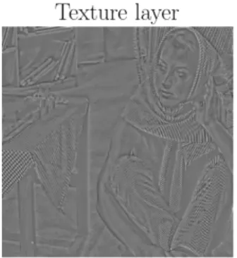
5.4 Cartoon+Texture Variational Image Decomposition
The next image processing example we consider is that of decomposing an imagey=u+v
into a cartoon-like componentuand a texture componentv(here we assume that the image is not
noisy). The cartoon layerucaptures flat regions separated by sharp edges, whereas the texture
componentvcontains the high frequency oscillations. There are many existing models to perform
such a decomposition, in the following, we implement the model proposed by Y. Meyer [37,47]:
inf u,v ∫ Ω∥∇u∥2dx+α∥v∥G s.t. y=u+v where ∥v∥G = inf д∈L∞(Ω; R2) {∥ q д2 1+д22∥∞s.t.v =divд} (40)
Fig. 10. Cartoon-texture decomposition withα=2e-4
This model favors flat regions inudue to the use of the TV norm and oscillatory regions invsince
∥v∥Gincreases for characteristic functions. Following [47], we reformulate the model as: inf u,д ∫ Ω∥∇u∥2dx s.t. y=u+div(д) q д2 1+д22 ≤α (41)
The original image (512×512) is here represented on a triangular finite-element mesh of similar mesh size and we adopt a Crouzeix-Raviart interpolation foruand a Raviart-Thomas interpolation forд. The constrainty=u+div(д)is enforced weakly on the CR space. The implementation reads as:
1 prob = MosekProblem("Cartoon/texture decomposition") 2 Vu = FunctionSpace(mesh, "CR", 1)
3 Vg = FunctionSpace(mesh, "RT", 1) 4 u, g = prob.add_var([Vu, Vg]) 5
6 def constraint(l):
7 return [dot(l, u)*dx, dot(l, div(g))*dx] 8 def rhs(l):
9 return dot(l, y)*dx
10 prob.add_eq_constraint(Vu, A=constraint, b=rhs) 11 12 tv_norm = L2Norm(u) 13 tv_norm.set_term(grad(u)) 14 prob.add_convex_term(tv_norm) 15 16 g_norm = L2Ball(g) 17 g_norm.set_term(g, k=alpha) 18 prob.add_convex_term(g_norm) 19 20 prob.optimize()
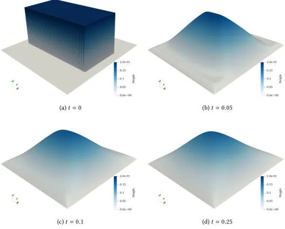
5.5 Time-dependent sandpile growth
In this example, we consider the time-dependent evolution model of a sandpile characterized by its heighth. Since sand can fall off the table domainΩ, Dirichlet boundary conditions are prescribed. Layers of sand having a slope larger than the critical angle at rest tanαwill fall down the slope and can be modelled by Prighozin evolutionary PDE [43]:
∂th−div(m∇h)=f inΩ× [0;T] (42)
m≥0, ∥∇h∥ ≤tanα m(∥∇h∥ −tanα)=0
withh(x,t)=0 forx∈∂Ωandh(x,0)=h0(x)as the initial sandpile height. In the above,−m∇h denotes the horizontal material flux of collapsing sand layers andf is a potential source term. This model has been also linked with the Monge-Kantorovitch problem of optimal mass transportation. Performing a backward implicit Euler discretization of the time derivative at each time steptn
and knowing the previous height configurationhn−1(x)at timet=tn−1, findinghn(x)amounts to
solving the following variational problem [24]:
inf h 1 2 ∫ Ω (h−дn)2dx s.t. ∥∇h∥ ≤tanα (43)
whereдn =∆t f +hn−1and∆t=T/Nis the time interval of eachNtime increments discretization of interval[0;T]. Adopting a standard LagrangeP1interpolation forh, problem (43) is solvedN
times with values ofдnupdated from the previous solution. Figure11illustrate the results obtained
withα =30◦, no source termf =0 and an initial unstable configuration forh
0since∥∇h0∥>tanα. 5.6 Optimal transport with space-time finite elements
Finally, we consider the Brenier-Benamou dynamic formulation [9] of quadratic cost optimal
transport between two distributionsρ0andρ1which reads as:
inf ρ,v 1 2 ∫ 1 0 ∫ Ωρ(x,t)∥v(x,t)∥ 2 2dx dt s.t. ∂tρ+divx(ρv)=0 ρ(x,t =0)=ρ0(x) ρ(x,t =1)=ρ1(x) v·n=0 on∂Ω (44)
The change of variable(ρ,m):=(ρ,ρv)proposed in [9] enables to obtain the following convex optimization problem: inf ρ,m ∫ 1 0 ∫ Ωc(ρ,m)dx dt s.t. ∂tρ+divxm=0 ρ(x,t=0)=ρ0(x) ρ(x,t=1)=ρ1(x) m·n=0 on∂Ω (45)
(a)t=0 (b)t=0.05
(c)t=0.1 (d)t=0.25
Fig. 11. Sandpile growth evolution starting from an initial unstable configuration (height amplification by factor 2)
where the cost function isc(ρ,m)=
∥m∥22 2ρ ifρ >0 0 if(ρ,m)=(0,0) +∞ otherwise
. This function is convex and,
ob-serving thatc(ρ,m) ≤tis equivalent to 2ρt ≥ ∥m∥22, is conic representable as follows: c(ρ,m)=min y y0 s.t. ρ m1 m2 − y1 y2 y3 =0 y∈ Qr4 (46)
The numerical approximation is performed by relying on a space-time finite element discretiza-tion ofQ =[0; 1]2× [0;T]withT =1. We adoptP2 Lagrange finite elements for the 3d-vector (ρ,m). Initial and boundary conditions are imposed on the different boundaries of the space-time cube. The mass conservation equation is replaced by a relaxed inequality between±ϵto allow for small deviations because of errors induced by the space-time discretization. It is written as:
1 prob = MosekProblem("Optimal transport") 2 u = prob.add_var(V, bc=bc)
3
4 conserv = InequalityConstraint(u, degree=2) 5 rho, mx, my = u[0], u[1], u[2]
6 eps = 1e-6
7 conserv.set_term(rho.dx(2)+mx.dx(0)+my.dx(1), bl=-eps, bu=eps) 8 prob.add_convex_term(conserv)
wheredx(0)anddx(1)stand for derivation along both spatial directions anddx(2)stands for
derivation along the third time direction. Finally, the cost function term is added following refor-mulation (46):
1 class CostFunction(ConvexFunction): 2 def conic_repr(self, X):
3 Y = self.add_var(dim=4, cone=RQuad(4))
4 Ybar = as_vector([Y[i] for i in range(1, 4)]) 5 self.add_eq_constraint([X, -Ybar]) 6 self.set_linear_term([None, Y[0]]) 7 8 c = CostFunction(u, degree=2) 9 c.set_term(u) 10 prob.add_convex_term(c)
Numerical results forρ(x,t)at different time slicestare represented in Figure12forρ0being a Gaussian distribution of standard deviation 0.2 andρ1being four identical Gaussian distributions of standard deviation 0.1 located on four opposite points of[0; 1]2. It can be observed how the optimal transport splits the initial distributionρ0into four parts driving towardsρ1.
6 CONCLUSIONS AND PERSPECTIVES
With the Python packagefenics_optimbased on the FEniCS project, we propose a way to
easily formulate convex variational problems arising in many applications of applied mathematics, image processing or mechanics. Convex optimization problems are formulated to fit into the conic programming framework in order to use efficient interior-point solvers especially tailored for such classes of problem. In the current form of the project, we use Mosek as the interior-point solver but other solvers could well be interfaced with the obtained discrete problems. The key point for fitting into the conic programming framework relies on a conic reformulation of convex functions.
We have shown that many elementary convex functions such asLpnorms arising in applications
can be indeed reformulated in such a way. In the gallery of examples we tackled, we showed
that various problems can be formulated with thefenics_optimlibrary in a very condensed
manner. Besides, despite the fact that interior-point solvers are not necessarily the method of choice for all the considered examples, in particular for image processing applications, they are still very efficient and robust. They are therefore a good choice for a general-purpose solver for the present package. Finally, the versatility of FEniCS in terms of discretization solutions allowed to formulate very easily different discretization strategies, in particular including DG finite-elements orH(div)-conforming elements which naturally arise in dual problems.
Obviously, there exist many aspects for improving the scope of the library or its efficiency. In
particular, the current implementation offenics_optimdoes not allow for problems involving
SDP matrix variables (Semi-Definite Programming problems), there are important applications in 3D computational mechanics which would benefit from such a feature. Besides, since version 9
(a)t=0:ρ0distribution (b)t =0.2 (c)t=0.4
(d)t=0.6 (e)t=0.8 (f)t=1:ρ1distribution
Fig. 12. Optimal transport between two distributions
of Mosek, power and exponential cones [19] are also available, which would broaden even more
the class of conic representable functions including, for instance,Lp-norms withp < {1,2,∞},
exponential, entropy functions, etc5. Including such a feature would therefore be a huge added value for many applications.
As regards computational efficiency, we mentioned that interior-point solvers, although being efficient and robust, have important memory requirements for large-scale problems since they rely on solving Newton-like systems using direct solvers. Image processing applications usually rely on proximal algorithms for solving the corresponding optimization problems, it would therefore be interesting to implement such algorithms in the package. Finally, there are some internal limitations due to the current status of the FEniCS library (e.g. Lagrange multipliers cannot be defined on one sub-part, the boundary for instance, of the domain) that could be improved. Fortunately, the FEniCS project is currently experiencing a major redevelopment to bring new functionality and improve efficiency6. We will therefore aim at taking advantage of these new developments in the
later versions of thefenics_optimpackage.
ACKNOWLEDGMENTS
The author would like to thank Gabriel Peyré for his useful advices when preparing the manu-script and F. Bleyer for providing some of the illustrative examples input material.
5seehttps://docs.mosek.com/modeling-cookbook/index.html
A GENERAL PRINCIPLES OFFENICS_OPTIMINTERNAL STRUCTURE A.1 Block-structure of the problem
The formulation of an optimization problem usingfenics_optimrelies on a block-structure
definition of variables and constraints. Let us consider, for instance formulation (24). The conic reformulation leads to the introduction of variablesbyin addition tou. Problem (24) therefore contains a block-structure ofp =2 variables(x1,x2)=(u,
by) ∈R
N ×
R4M. The internal machinery
offenics_optimworks by adding sequentially new optimization variables, possibly associated with bound or conic constraints, and new linear equality or inequality constraints. Pseudo-code for defining such a block-wise structure would look like:
1 # Problem initialization
2 prob = MosekProblem("My problem") 3
4 # Adding a first block variable x1
5 x1 = prob.add_var(V1, lx=lx1, ux=ux1, cone=K1) 6 # Adding a first linear constraint
7 prob.add_ineq_constraint(W1, A=[a1], bl=bl1, bu=bu1)
At this stage, theprobinstance represents the following problem:
min x1∈V1 0 s.t. l1 x ≤x1 ≤u1x b1 l ≤A1x1 ≤b1u (47)
whereV1would beRd1in a purely discrete setting but will, in fact, be the variableFunctionSpace
in the FEniCS FE-discretization setting. Bounds likel1x,u1x,b1l,b1u are ±∞ by default (None in
Python) and can be ignored in such case.K1 is a Coneobject describing the type of cone to
which the variable belongs (againNoneby default if there is no conic constraint). Finally, the
linear constraint matrixA1is represented by a bilinear forma1(y1,x1)onW1×V1wherey1is the constraint Lagrange multiplier andW1its correspondingFunctionSpace. The bilinear forma1is then assembled by FEniCS to produce the discrete matrixA1stored in sparse format.
Adding a second variable is then similar, except that constraints must now include the block-structure of both variables such as:
1 # Problem initialization
2 prob = MosekProblem("My problem") 3
4 # Adding a first block variable x1
5 x1 = prob.add_var(V1, lx=lx1, ux=ux1, cone=K1) 6 # Adding a first linear constraint
7 prob.add_ineq_constraint(W1, A=[a1], bl=bl1, bu=bu1) 8
9 # Adding a second block variable x2
10 x2 = prob.add_var(V2, lx=lx2, ux=ux2, cone=K2) 11 # Adding a second linear constraint
where we now have two bilinear formsa21(y2,x1)onW
2×V1anda22(y2,x2)onW2×V2leading to: min (x1,x2)∈V 1×V2 0 s.t. l1x ≤x1≤u1x b1l ≤A1x1≤bu1 l2 x ≤x2≤u2x b2 l ≤A21x1+A22x2≤bu2 (48)
Finally, a linear objective term(c1)Tx1+(c2)Tx2can be added as
1 prob.add_obj_fun([c1, c2])
The final block-structure for a problem withpblocks will therefore look like: min x=(x1,...,xp)∈V1×...×Vp (c1, . . . ,cp)T(x1, . . . ,xp) s.t. lx ≤x≤ux bl ≤ A11 0 . . . 0 A21 A22 . . . 0 .. . ... . .. ... Ap1 Ap2 . . . App x≤bu (49)
Note that when defining sequentially the block-constraints until variablexi, the blocksAijwith j >iare automatically zero since variablesxjhave not been defined yet. This is by no means a restriction since one could perfectly define the constraint matrices once all variables have been defined. This lower-triangular structure allows however for an easier definition of the constraints
in many cases. Note also that empty blocks can also be written with0orNonein Python. Such
symbols must be explicitly used for allAijwithj≤i. A.2 Explicit construction of problem(24)
Going back to problem (24), one could do first:
1 # Problem initialization
2 prob = MosekProblem("Obstacle problem") 3
4 # Adding a first block variable u 5 u = prob.add_var(Vu, lx=g)
creating only variableuand its lower bound constraintu≥g.
Auxiliary variablebycorresponds to a 4-dimensional vectorial field with degrees of freedom located
at quadrature points. FEniCS provides such a functional space through the concept ofQuadrature
elements. We will use one, notedV2, of dimension 4 forbyand one, notedW, of dimension 3 for the Lagrange multipliers corresponding to constraints:
yд,1=1 Bдu− y д,2 yд,3 =0
Indeed, satisfying the above constraints for all Gauss pointsдis equivalent to writing:
where a12(z,u)=∫ Ω z 2 z3 · ∇udx a22(z,y)=−∫ Ωz ·© « y1 y2 y3 ª ® ¬ dx b(z)= ∫ Ωz· © « −1 0 0 ª ® ¬ dx
in which the integrals are computed using the same quadrature used for definingy∈V2andz∈W. This results in the following code:
1 def quad_element(degree=0, dim=1):
2 return VectorElement("Quadrature", mesh.ufl_cell(), 3 degree=degree, dim=dim, quad_scheme="default") 4 V2 = FunctionSpace(mesh, quad_element(degree=0, dim=4)) 5 W = FunctionSpace(mesh, quad_element(degree=0, dim=3)) 6 y = prob.add_var(V2, cone = RQuad(4))
7
8 dxq = Measure("dx", metadata={"quadrature_scheme":"default", 9 "quadrature_degree":0})
10 def constraint(z): 11 g = grad(u)
12 a21 = dot(z, as_vector([0, g[0], g[1]]))*dxq 13 a22 = -dot(z, as_vector([y[1], y[2], y[3]]))*dxq 14 return [a21, a22]
15 def rhs(z):
16 return -z[0]*dxq
17 prob.add_eq_constraint(W, A=constraint, b=rhs)
wherey ∈V2 is created by specifying that it also belongs to a rotated quadratic coneQr4. This
statement is understood point-wise, meaning that at each degree of freedom (Gauss point) location xд, the local 4-d vectory(xд)belongs to Qr4. Thedxqmeasure is used to enforce a one-point quadrature on each cell, the same used for the definition ofV2andW. Finally, the constraint matrix
is passed as a function (constraint) of the Lagrange multiplierz ∈ W and returns a list of 2
bilinear forms corresponding to both blocks inuandy, while the constraint right-hand side is also passed as a function ofz(rhs) and returns a single linear form inz. A similar syntax would be used for inequality constraints.
Finally, the objective term is set as a list of two linear forms inuandyrespectively:
1 prob.add_obj_func([-dot(load, u)*dx, y[0]*dxq])
Note again the use of the one-point quadrature measure for the second term.
One role ofConvexFunctionclasses described in3.3is to avoid for the user to explicitly define function spaces for the additional variables and Lagrange multipliers. The complete script of this
B CONIC REFORMULATION OF PROBLEM(36) We consider functionπ :M ∈S2←→ 2√m 3 q M2 11+M222+M122 +M11M22. ExpressingM ∈S2as X=(M11,M22,2M12), we have that: π(M)=bπ(X)=√m 3 p XTCXwithC= 4 2 0 2 4 0 0 0 1 (51)
Computing the Cholesky factorJ=
2 1 0 0 √3 0 0 0 1
of matrixC, we have thatbπ(X)=√m
3 p XTJTJX= m √ 3∥JX∥2. REFERENCES
[1] Alnæs, M. S. (2012).UFL: a Finite Element Form Language, chapter 17. Springer.
[2] Alnæs, M. S., Blechta, J., Hake, J., Johansson, A., Kehlet, B., Logg, A., Richardson, C., Ring, J., Rognes, M. E., and Wells, G. N. (2015). The fenics project version 1.5.Archive of Numerical Software, 3(100).
[3] Alnæs, M. S., Logg, A., Ølgaard, K. B., Rognes, M. E., and Wells, G. N. (2014). Unified form language: A domain-specific language for weak formulations of partial differential equations.ACM Transactions on Mathematical Software, 40(2). [4] Andersen, E. D., Roos, C., and Terlaky, T. (2003). On implementing a primal-dual interior-point method for conic
quadratic optimization.Mathematical Programming, 95(2):249–277.
[5] Balay, S., Abhyankar, S., Adams, M. F., Brown, J., Brune, P., Buschelman, K., Dalcin, L., Eijkhout, V., Gropp, W. D., Kaushik, D., Knepley, M. G., McInnes, L. C., Rupp, K., Smith, B. F., Zampini, S., Zhang, H., and Zhang, H. (2016). PETSc Web page. http://www.mcs.anl.gov/petsc.
[6] Balmforth, N. J., Frigaard, I. A., and Ovarlez, G. (2014). Yielding to stress: recent developments in viscoplastic fluid mechanics.Annual Review of Fluid Mechanics, 46:121–146.
[7] Ben-Tal, A., El Ghaoui, L., and Nemirovski, A. (2009).Robust optimization, volume 28. Princeton University Press. [8] Ben-Tal, A. and Nemirovski, A. (2002). Robust optimization–methodology and applications.Mathematical Programming,
92(3):453–480.
[9] Benamou, J.-D. and Brenier, Y. (2000). A computational fluid mechanics solution to the Monge-Kantorovich mass transfer problem.Numerische Mathematik, 84(3):375–393.
[10] Bendsoe, M. P. and Sigmund, O. (2004).Topology Optimization: Theory, Methods and Applications. Springer. [11] Bleyer, J. (2018). Advances in the simulation of viscoplastic fluid flows using interior-point methods.Computer Methods
in Applied Mechanics and Engineering, 330:368–394.
[12] Bleyer, J., Carlier, G., Duval, V., Mirebeau, J.-M., and Peyré, G. (2016). Aγ-convergence result for the upper bound limit analysis of plates.ESAIM: Mathematical Modelling and Numerical Analysis, 50(1):215–235.
[13] Bleyer, J. and de Buhan, P. (2013). On the performance of non-conforming finite elements for the upper bound limit analysis of plates.International Journal for Numerical Methods in Engineering, 94(3):308–330.
[14] Bleyer, J., Maillard, M., De Buhan, P., and Coussot, P. (2015). Efficient numerical computations of yield stress fluid flows using second-order cone programming.Computer Methods in Applied Mechanics and Engineering, 283:599–614. [15] Capsoni, A. and Corradi, L. (1999). Limit analysis of plates- a finite element formulation.Structural Engineering and
Mechanics, 8(4):325–341.
[16] Carlier, G., Comte, M., Ionescu, I., and Peyré, G. (2011). A projection approach to the numerical analysis of limit load problems.Mathematical Models and Methods in Applied Sciences, 21(06):1291–1316.
[17] Carlier, G., Comte, M., and Peyré, G. (2009). Approximation of maximal cheeger sets by projection.ESAIM: Mathematical Modelling and Numerical Analysis, 43(1):139–150.
[18] Chambolle, A. and Pock, T. (2018). Crouzeix-raviart approximation of the total variation on simplicial meshes. hal-01787012.
[19] Chares, R. (2009).Cones and interior-point algorithms for structured convex optimization involving powers andexponentials. PhD thesis, Ph. D. Thesis, UCL-Université Catholique de Louvain, Louvain-la-Neuve, Belgium.
[20] Cheeger, J. (1969). A lower bound for the smallest eigenvalue of the laplacian. InProceedings of the Princeton conference in honor of Professor S. Bochner.
![Fig. 7. Horizontal velocity profile u x ( y) on the middle plane x = 0.5, comparison with results from [14]](https://thumb-us.123doks.com/thumbv2/123dok_us/10116362.2912185/20.729.75.657.134.356/fig-horizontal-velocity-profile-middle-plane-comparison-results.webp)