Improving flood prediction using data assimilation

(1)

UNIVERSITY OF READING

Department of Meteorology

Improving flood prediction using

data assimilation

Elizabeth S. Cooper

A thesis submitted for the degree of Doctor of Philosophy

(2)

Declaration

I confirm that this is my own work and the use of all material from other sources has

been properly and fully acknowledged.

(3)

Publications

Chapters 4 and 5 of this thesis are reproduced from the following publications

re-spectively:

• Cooper, E. S., Dance, S. L., Garcia-Pintado, J., Nichols, N. K. and Smith, P. J.

Observation impact, domain length and parameter estimation in data assimilation

for flood forecasting. Environmental Modelling and Software, 104. pp. 199-214. ISSN 1364-8152, https://doi.org/10.1016/j.envsoft.2018.03.013 (2018)

• Cooper, E. S., Dance, S. L., Garca-Pintado, J., Nichols, N. K., and Smith, P.:

Observation operators for assimilation of satellite observations in fluvial inundation forecasting, Hydrol. Earth Syst. Sci. Discuss., https://doi.org/10.5194/hess-2018-589, in review, 2018.

All work undertaken in these publications was carried out by Elizabeth Cooper with

(4)

Abstract

River flooding is a costly problem worldwide. Timely, accurate prediction of the

behaviour of flood water is vital in helping people make preparations. Mathematical hydrodynamic models can predict the behaviour of flood water given information about

inputs such as river bathymetry, local topography, inflows, and values for model parame-ters. Uncertainty in these inputs leads to inaccuracies in model predictions; data

assimila-tion can be used to improve forecasts by combining model predicassimila-tions with observaassimila-tional information, taking into account uncertainties in both.

In this thesis we investigate ways to maximize the impact of observational infor-mation from satellite-based synthetic aperture (SAR) instruments in data assimilation

for inundation forecasting. We show in synthetic twin experiments using an ensemble transform Kalman filter that using joint state-parameter data assimilation techniques to

correct the model channel friction parameter as well as water levels provides a significant, long lasting benefit to the model forecast. We show that errors in the channel friction

parameter and inflow are interdependent.

We propose a novel observation operator that allows direct use of measured SAR backscatter values, potentially allowing the use of many more observations per SAR

im-age. We test our new observation operator in synthetic experiments, showing that we can successfully update inundation forecasts and the value of the model channel friction

pa-rameter using our new approach. We show that different observation operator approaches can generate significantly different updates to model forecasts and illustrate the

physi-cal mechanisms responsible. Lastly, we use our new observation operator to assimilate backscatter values from real SAR images, showing that our new approach can be used to

improve inundation forecasts in a real case study. Improved understanding of the physical mechanisms by which updates are generated by different observation operators provides

(5)

Dedication

(6)

Acknowledgements

I would like to thank my team of excellent supervisors, Prof. Sarah Dance, Dr. Polly

Smith, Prof. Nancy Nichols and Dr. Javier Garcia-Pintado for huge amounts of support and encouragement. I would also like to thank David Mason for some really helpful

input at various stages of the project. I gratefully acknowledge financial support from the National Environmental Research Council (NERC) through the SCENARIO DTP, and

from my CASE sponsors the Satellite Applications Catapult.

The Meteorology Department at Reading has been a great place to study and I’m

grateful to everyone I’ve had useful discussions and tea breaks with over the last 4.5 years. Special thanks to members of DARC, to current office-mates Aga, Michael and Kaja, and

to Hannah Bloomfield who has been a marvel.

Lastly I want to thank my wonderful family, especially my Mum and Dad, for their endless support. Massive thanks to Mum and Fran for looking after the boys while I

worked; without your help I couldn’t possibly have done this. And thanks to Richard for so many things, including encouragement, laughter, sympathy and wine. Finally, thank

(7)

Contents

Introduction

1.1 Motivation

River flooding is a costly problem in the UK and worldwide (e.g. Ward et al. [2018])

and the number of people exposed to flood risk is expected to increase with future cli-mate change (see e.g. Yamazaki et al. [2018]). Real-time, accurate inundation forecasts

from numerical models can help to mitigate the damage caused by river inundation events by alerting people to when and where they are likely to be affected. However,

predic-tions from such numerical inundation models are inevitably subject to uncertainty due to approximations in the governing equations and uncertainties in model parameters and

driving data. The work in this thesis is part of an effort to improve inundation forecasts using data assimilation, a powerful mathematical tool which can be used to combine

predictions from a numerical inundation model with observations in order to give better predictions of flood extent and depth. In particular, the work in this thesis explores

ques-tions about how to make the best use of observational information. We wish to maximise the observation impact of SAR-derived information, i.e. we seek to improve the accuracy

of inundation forecasts but also to increase the time over which the observations influence the forecast.

A number of authors have used data assimilation to improve inundation forecasting in a number of different ways, as we discuss in chapter 2. Some studies (e.g. Ricci et al.

[2011], Lai and Monnier [2009] and Hostache et al. [2010]) have focussed on using obser-vational information from river gauges, either alone or in combination with information

from satellite images; in this thesis we consider situations in which synthetic aperture radar (SAR) observations are our only source of information. SAR has the advantage

(11)

Chapter 1: Introduction

cover or rain, which could otherwise cause problems in flood situations. The reason for taking a SAR-only approach is that the number of gauges worldwide is in decline

(Vrs-marty et al. [2001]) and we wish to have a method that will be applicable in ungauged catchments. Although SAR observations typically show a clear delineation between wet

and dry areas, and can cover a large spatial area, the information they contain is limited in time. Using SAR-based information to correct only water levels can therefore lead

to short-lived improvement in the forecast. Some authors (e.g. Andreadis et al. [2007], Matgen et al. [2010], Giustarini et al. [2011], Garcia-Pintado et al. [2015], Garcia-Pintado et al. [2013] and Mason et al. [2015]) have demonstrated increased observation impact

by correcting errors in inflow (amount of water flowing into the domain of interest) as well as water levels, but less attention has been paid the role of model parameters. It is

well known that channel friction processes are important in the evolution of flood events (e.g. Hostache et al. [2010], James et al. [2016]) and in this thesis we therefore investigate

whether using data assimilation to correct the value of the parameter controlling channel friction can increase observation impact.

There are a number of ways in which information from a SAR image could be used in

data assimilation. Authors such as Neal et al. [2009], Giustarini et al. [2011], Giustarini et al. [2012] and Garcia-Pintado et al. [2015] have used SAR-derived water levels as

observations. This involves intersecting SAR images with digital elevation models in order to extract information about water level. Such observations are typically sparse in real

case studies (e.g.Mason et al. [2012]). We have designed and implemented a new approach to extracting information from SAR images, in which we directly use measured backscatter

values as observations. This approach allows for the use of many more observations than the derived water level approach and requires less processing of the SAR image,

potentially speeding up the time taken between acquisition and an updated forecast. A related approach is used in Hostache et al. [2018], in which the authors use SAR images to produce flood probability maps and use these as observations in a particle filtering

method.

1.2 Thesis aims

The aims of this thesis are to answer the following research questions:

1. How does estimation of the channel friction parameter affect observation impact in data assimilation for inundation forecasting?

(12)

Can we use joint state-parameter data assimilation techniques to retrieve the correct channel friction parameter in synthetic experiments using SAR-like observations,

and does this significantly improve the forecast? How is error in the channel friction parameter related to error in inflows?

2. Can we design and implement a new method of extracting observational information from a SAR image for use in data assimilation?

How do existing approaches generate an update to the forecast via the observation operator? Can we design and implement a new observation operator in order to

use raw backscatter observations in data assimilation? Does our new observation operator work to improve the forecast in synthetic experiments, and can we use it

to recover the true value of the channel friction coefficient?

3. Can we apply our new observation approach to a case study using real topography and SAR data?

Does our new backscatter observation operator improve the forecast in a real case study, and do we observe the same physical mechanisms as in the synthetic

ex-periments? How can we measure improvement to the forecast when we have no synthetic ‘truth’ to compare to?

1.3 Principal new results

The work in this thesis provides the following answers to the research questions posed:

1. In our synthetic experiments using a simplified domain we found that it was possi-ble to retrieve the correct value for the channel friction parameter using synthetic

SAR-derived water level observations in a joint state-parameter data assimilation approach. We found that correcting the channel friction parameter has a large,

positive impact on subsequent water depth forecasts, significantly improving obser-vation impact by extending the time over which obserobser-vations influence the forecast.

We found that inflow error and channel friction parameter error are interdependent, making the two sources of error difficult to separate out.

2. We have designed and implemented a new observation operator that directly uses SAR backscatter values as observations. We have shown that the method can be

used to successfully update a model forecast and concurrently correct the value of the channel friction parameter in synthetic experiments. We have shown that

(13)

Chapter 1: Introduction

different approaches to observations from SAR images (water level observations vs backscatter observations) and different observation operators can produce

sub-stantially different updates to modelled inundation predictions. We explain these differences by illustrating the physical mechanisms responsible for the updates in

the different approaches.

3. We successfully applied our novel backscatter observation operator to a real case study, using a series of SAR images capturing a flood event near Tewkesbury in

the UK in the winter of 2012. We used a series of binary flood match measures to demonstrate the benefit to the forecast of updating water levels in this way.

1.4 Thesis outline

This thesis is structured as follows:

• Chapter 2 outlines the principles of data assimilation for inundation prediction, and

describes the work of other authors in approaching this problem. We briefly describe SAR measurements and approaches to inundation modelling.

• Chapter 3 introduces and describes the Clawpack software that was used to build

our inundation model and run all of the inundation simulations in this thesis.

• Chapter 4 addresses the first research question posed in section 1.2. We describe

a series of synthetic experiments in which we show that we can use joint

state-parameter estimation techniques to successfully retrieve a good value for the channel friction parameter, and that this has a significant impact on the forecast. We also

show that assuming zero momentum immediately following an assimilation causes a shock in the solution and demonstrate a simple method for avoiding this problem.

This chapter has been published as Cooper et al. [2018b].

• Chapter 5 addresses the second research question. We outline two existing methods

that can be used to assimilate SAR-derived flood edge water elevation measures. We then introduce a novel method which directly assimilates backscatter values from a

SAR image. We describe the three different observation operators and show that the choice of observation operator can have large impact on the updated inundation

forecast. We compare the results of using the three different operators in synthetic experiments and discuss the physical mechanisms associated with generating an

(14)

• Chapter 6 addresses the final research question and shows the results of applying our

new observation operator (described in chapter 5) to a real case study. We show that

assimilating SAR-derived backscatter values generates an update to model predicted water levels, and that this update improves the forecast at the assimilation time.

• Chapter 7 summarizes the main conclusions of the thesis and outlines possible areas

(15)

Chapter 2: Data assimilation for inundation forecasting

Chapter 2:

Data assimilation for inundation

forecasting

In this chapter we introduce some of the key topics used in this thesis. In section 2.1 we briefly outline the theory of data assimilation. In section 2.2 we discuss approaches to

fluvial inundation modelling; in section 2.3 we introduce the Synthetic Aperture Radar (SAR) images used to provide observations for data assimilation in this thesis. We

sum-marise a number of current approaches to data assimilation for inundation forecasting in section 2.4. In section 2.5 we introduce the forecast verification measures that are used

in chapter 6 to assess the agreement between inundation model predictions and observed data.

2.1 Introduction to data assimilation

Data assimilation is a powerful mathematical technique in which predictions from

a numerical model of a dynamical physical system are combined with observational in-formation; this allows us to predict the current and future states of the physical system

more accurately than using either a numerical model or observations in isolation. In this thesis we consider river flooding, but data assimilation methods are very well established

in operational numerical weather prediction (e.g. Rawlins et al. [2007]) and are employed in a wide variety of applications including modelling of land surface processes, (e.g.

Pin-nington et al. [2018]), ocean modelling (e.g. Thomas and Haines [2017]) and neuroscience (e.g. Moye and Diekman [2018]).

In data assimilation we describe the evolution of a dynamical physical process, such as a flood event, using a forecast model,

(16)

x(tk+1) =M(x(tk)), (2.1) where x ∈ _RN _{is the model state vector,} _t _{represents time and} _M _:

RN → RN is the

forecast model; in this case an inundation model.

We assume that at particular times we have observations of the system, y_obs ∈ _Rp_, related to the true state,xt, by

y_obs =h(xt) +. (2.2)

Observations may be indirect measurements of state variables and not located at model

cell centres, so an observation operator,h:RN →Rp is required to map the state vector

into observation space. Observation noise, , is assumed to be Gaussian, stochastic and

unbiased, with covarianceR∈Rp×p.

There are a number of approaches to the data assimilation problem, in which we

seek the state (called the ‘analysis’) that best matches both the model prediction and the observations, subject to the uncertainties in each. One approach is to minimize a cost

function of the form

J(x) = 1 2(x−x f₎_P−1₍_x₋_xf_{) +}1 2(yobs−h(x f₎₎_R−1₍_y obs−h(xf)), (2.3) wherexf is the model prediction at the observation time (often called the ‘background’ state and referred to in this thesis as the ‘forecast’ state). The matrix P ∈ RN×N is

the forecast error covariance matrix, and R ∈ _Rp×p _{is the observation error covariance} matrix. Minimisation of equation 2.3 corresponds to the maximum a posteriori (MAP) solution. The MAP is equivalent to the minimum variance solution when h and M are linear, under the assumption that the errors in the forecast state and observations are

Gaussian (Nichols [2010]). The first term on the right hand side of equation 2.3 describes the difference between the model state and the forecast state, the second term describes

the difference between the model state and the observations, and these terms are weighted according to the relative uncertainties in the forecast and the observations throughPand

(17)

2.1.1 Variational approaches

In variational data assimilation, the cost function is minimised using numerical it-erative methods. Variational techniques generally use the same forecast error covariance

matrix at all assimilation times, i.e. uncertainty in the forecast state is assumed to be fixed and not updated based on observational information. The sequential variational

approach is known as 3D-Var (e.g. Lorenc et al. [2000]). Sequential data assimilation schemes comprise two steps: a forecast step in which the system is evolved according to

equation 2.1 and an update step, in which we update the model forecast according to the observations. The updated (analysis) state is then used as the starting point for the next

forecast step and the process can be repeated many times. An alternative to the sequen-tial approach is the 4D-Var approach (e.g. Rawlins et al. [2007]), in which an assimilation

time window is defined. In 4D-Var techniques, the aim is to find the initial state which best fits the forecast state at the initial time (the background) and all of the observations

available in the defined window, subject to the model equation 2.1. The advantage of the 4D-Var approach is that observations can be distributed across an assimilation window.

2.1.2 Kalman filter approaches

The Kalman filter (KF) (Kalman [1960]) provides a solution that minimises equation

2.3 in systems with linear forecast models and observation operators. An advantage of the Kalman filter approach over variational methods is that the forecast state error covariance

matrix is updated at each assimilation time along with the model state. The Kalman filter is only applicable to systems with linear h and M; the extended Kalman filter (EKF) is an approximation to the KF which can be used in the case of non-linearity. The EKF

requires linearisation of the observation operator and forward model; this can lead to poor results in highly non-linear cases (Gelb [1974]).

2.1.3 Ensemble Kalman filter approaches

In this thesis we use an ensemble transform Kalman filter (ETKF) to find the analysis

state. The ETKF is a sequential technique, based on the Kalman filter, which uses an ensemble of state vectors to represent a number of possible realisations of the dynamic

system. There are a number of different ensemble Kalman filter (EnKF) methods but in all of them the ensemble mean is used to represent the best estimate of the true

(18)

estimate of the uncertainty in the mean prediction ([Evensen, 1994]). One formulation of the EnKF uses perturbed observations to ensure that the analysis ensemble retains the

correct statistics (Evensen [2003]); we have used an ETKF which is sometimes known as a ‘deterministic’ EnKF method as it does not require observation perturbations. Variants

of the deterministic approach are reviewed in Tippett et al. [2003]. The ETKF is one of a number of square root filters, which are reviewed in Livings et al. [2008]. We use an

ETKF here following the approach of Garcia-Pintado et al. [2013] and Garcia-Pintado et al. [2015] for a similar application. The ETKF has the advantage of being numerically efficient in implementation.

The ETKF is valid for non-linear forecast models and observation operators, and

retains the advantage of flow-dependent forecast state covariances. However, since the ensemble is a statistical sample of state space, there are a number of potential problems

with practical implementation of the technique. Undersampling can lead to underesti-mation in ensemble spread (ensemble collapse), causing the forecast to give insufficient

weight to observations and diverge from the truth (filter divergence)(Petrie and Dance [2010]). Inflation techniques can be used to counter this problem (see e.g. Anderson

[2007]). Undersampling can also lead to noise in the state forecast covariance matrix, producing spurious updates (Petrie and Dance [2010]). Techniques to deal with this

problems include localization (e.g. Hamill et al. [2001]). The Kalman filter and ETKF update equations are given in section 4.3.2.

2.1.4 Particle filter approaches

Particle filter techniques represent another sequential approach to the data assimila-tion problem (e.g. van Leeuwen [2009], Doucet et al. [2013]). In particle filter methods the

requirement for errors to be Gaussian is relaxed, and non-linear models and observation operators are permitted. Particle filter approaches use an ensemble of states, or particles,

to represent forecast and analysis uncertainty in a similar way to EnKF systems. Standard particle filter techniques are known to suffer from problems such as particle degeneracy

and impoverishment, particularly when the size of the state is large (e.g. Snyder et al. [2008]).

(19)

2.2 Inundation models

In this section we discuss some approaches to modelling river flood inundation pro-cesses. In chapter 3 we discuss in more detail the particular hydrodynamic model used

in the remainder of this thesis, which uses Clawpack software (Clawpack Development Team [2014]).

There are a number of well developed numerical inundation models that can predict the behaviour of flood water given information about the topography of the domain and

the amount of water flowing into the area, e.g. HEC-RAS [HEC-RAS Development Team], Telemac [Hervouet, 2000], LISFLOOD-FP [Neal et al., 2012a], Dassflow [Honnorat et al.,

2007]. Most models use a variation of the shallow water equations to predict changes in water depth in river channels. The shallow water equations are an approximation to the

Navier-Stokes equations, which can be used to model the behaviour of fluids. The shallow water equations are valid for situations in which

• the vertical scales are much smaller than the horizontal scales, allowing vertical

velocity to be neglected;

• viscous forces can be neglected;

• the fluid being modelled is incompressible.

These approximations are generally met for inundation modelling applications. The shal-low water equations are given and discussed in the context of Clawpack in section 3.1.

Hydrodynamic inundation models provide approximate solutions to the shallow

wa-ter equations using various numerical schemes. Models can use implicit methods (using information from the current time as well as the past time to calculate a solution) or

ex-plicit methods (which use information from past timesteps only to calculate the solution). HEC-RAS and Telemac-2d use implicit methods, whereas Clawpack and LISFLOOD-FP

use explicit solvers. Time steps in the model can be user-specified or can be adaptive to preserve numerical stability. Models can solve 1D or 2D forms of the shallow water equations, and use a variety of discretisation approaches. HEC-RAS uses finite

differ-ence methods to solve the full 1D shallow water equations in river channels and makes assumptions about the conveyance of water onto the floodplain. Telemac-2d uses finite

volume methods to to solve the 2D depth-averaged shallow water equations. Dassflow has both 1D and 2D capabilities and uses finite volume methods on an unstructured mesh.

(20)

equations in river channels and a raster-based approach on the floodplain.

The 1D approach is considerably less expensive than using the full 2D shallow water

equations, but has the disadvantage that momentum is not exchanged between water in the river and on the floodplain. Three different model approaches are compared in Horritt

and Bates [2002], in which HEC-RAS (1D), LISFLOOD-FP (1D and raster approach) and Telemac-2d (2D) are all separately calibrated for two flood events of the river Severn, UK,

two years apart. The predictions of models calibrated on the first flood are then compared with satellite-derived inundation extents from the second flood and vice versa. The study

shows that the three models all had similar predictive power when optimally calibrated, but that the performance of LISFLOOD-FP was sensitive to the type of calibration data

used, requiring calibration against inundation data rather than discharge data to give good results. In Neal et al. [2012b] the authors use a series of benchmarking tests to compare the

performance of three different approaches to solving the 2D shallow water equations, and show that for gradually varying flows the simplest representation of the physical processes

performed similarly well to more complex representations, and to industry standards for commercial inundation codes. However, simpler models are unable to deal with shocks

(hydraulic jumps). In the hydrodynamic model we use for the simulations in this thesis we use a finite volume, explicit method to solve the 2D shallow water equations throughout

the domain. Our method is able to simulate shocks in the solution.

Numerical models require appropriate boundary conditions in order to generate

re-alistic solutions, and there are a number of different approaches to specifying these. In many models it is possible to set an inflow rate at the upstream boundary, which can

be based on measured gauging station data. A downstream boundary condition can be set by specifying the water depth at the boundary, or an outflow rate; either of these

conditions may be available from gauging stations. In our work we use an extrapolating outflow boundary, to allow water to freely leave the domain (see section 3.1.2 for more

details of the boundary condition options in Clawpack); we treated inflow as a source term in the equations (see section 4.8.2).

In inundation modelling, the boundary between wet and dry areas on the floodplain moves as the flood event develops and this moving boundary can cause problems for some

solvers. Approaches that use the 1D equations do not suffer from this problem as the shallow water equations are only valid in the channel with e.g. a 2D or raster-based

volume filling approach on the floodplain. Clawpack deals with the problem of wet/dry interfaces by assuming that there is water everywhere in the domain, but that the water

(21)

depth is zero in dry areas.

All inundation models require good topographical information to give accurate

re-sults. Digital Terrain Models (DTMs) are often available for flood plains, although are not always of a sufficiently high quality for hydrological modelling (see Schumann and

Bates [2018]). DTMs do not typically contain information about river and stream bed elevations, and accurate, recent representation of river channels can be difficult to obtain.

Further, combining information about flood plain and river topography is non-trivial. When high resolution topography information is available, the resolution at which the

model is run will depend on the available compute resources; higher resolution models provide more accurate results but at a higher cost and a longer run time. To address

this problem, LISFLOOD-FP uses a sophisticated sub-grid parameterization technique for river channels, allowing accurate representations of flow in river channels with

dimen-sions smaller than the grid-scale (see Neal et al. [2012a]); this reduces the cost of the model by removing the need for a grid resolution that can resolve river channels.

2.3 Synthetic aperture radar (SAR) observations

Synthetic Aperture Radar instruments on satellites (such as CosmoSkymed and

Sen-tinel 1) can provide a large amount of observational information about a river flood event (e.g. Brown et al. [2016], Schumann et al. [2009], Mason et al. [2012]). SAR instruments

are side-looking active instruments that emit radiation (of wavelength cm to m) towards the surface of the Earth. SAR instruments use cloud penetrating radiation, giving the

instruments all-weather capability, and can be operational day and night, unlike passive sensors that rely on solar radiation. The strength of the returned signal measured at the

SAR sensor depends strongly on the roughness properties of the surface from which it has been reflected.

Figure 2.1 shows an example of a SAR image in a flood situation. Areas of open water are very smooth and therefore reflect a large proportion of the incoming radiation away

from the sensor. Pixels in flooded or other wet areas therefore have low backscatter values and appear as dark areas on SAR images. Dry areas have rougher surface properties and

reflect a larger proportion of incoming radiation back towards the sensor; dry areas have higher backscatter values and therefore appear paler than wet areas. During a flood event

SAR images therefore generally show a clear difference between flooded and non-flooded areas.

(22)

Figure 2.1: TerraSAR-X 2.5m resolution SAR image of the Severn catchment near Tewkes-bury, UK, July 2007. Reproduced from Mason et al. [2012]. Dark areas are water.

SAR images can be processed to various different levels of calibration. In chapter 6

we use digital number (DN) values for our observations, whereas in Giustarini et al. [2011], backscatter values measured in dB are used for data assimilation. When

purchas-ing SAR data, DN values are available at lower cost than backscatter values. This is because backscatter values are processed to a higher level than DN values; a radiometric

calibration is required to produce backscatter values. Radiometric calibration is essential when comparing SAR images taken at different times, but it is possible to use DN values

to identify wet and dry pixels contained in one particular image.

There are a number of approaches to identifying pixels as wet or dry based on SAR

backscatter or DN measurements. Techniques include thresholding (e.g. Henry et al. [2006]) with varying levels of user-interpretation (as compared in Brown et al. [2016])

and region growing/clustering (e.g. Horritt et al. [2001]); it is also possible to use change detection methods if a number of co-located images are available (e.g. Hostache et al.

[2012]). Identifying wet and dry areas using these methods can be used for flood mapping and monitoring (as in e.g. Brown et al. [2016], Matgen et al. [2011]) and for validation

and calibration of inundation models (e.g. Mason et al. [2009], Baldassarre et al. [2009] Wood et al. [2016]).

(23)

Intersection of flood edges with a DTM provides information about the elevation of water, by using the fact that water elevation must be the same as the terrain elevation at

the location of the flood edge. For model calibration, Mason et al. [2009] and Stephens et al. [2013] show that better calibration can be achieved by comparing modelled water

levels with SAR derived water levels, rather than using binary wet-dry comparisons. However, it is not clear whether derived water levels provide better observation impact

than wet/dry observations in data assimilation; this question is addressed in chapter 5.

A difficulty in determining flood edge water levels arises when a flood edge is found to

be on a steeply sloping area of topography, since small errors in pinpointing the position of the flood edge cause large errors in the elevation assigned to the water. Flood edges in

positions with slopes above a threshold are therefore often excluded from calculations e.g. Mason et al. [2012]. Complications in accurately determining the flood edge in a SAR

image can include:

• Vegetation: If the flooded area contains plants that are taller than the flood depth,

this can affect the SAR signal return strength, causing wet areas to appear dry.

• In windy conditions the surface of a body of water can be rough due to ripples and

therefore have a higher backscatter values than usual. This potentially risks wet

areas appearing to be dry.

• In urban areas, buildings can prevent substantial amounts of ground being observed

by SAR instruments due to layover and shadowing (see Mason et al. [2014], Mason

et al. [2018], Tanguy et al. [2017]).

2.4 Approaches to data assimilation for inundation

fore-casting

There have been a number of attempts to use data assimilation to improve

hydro-dynamic forecasting, many of which have used data from gauges to provide observational information. For example, in Madsen [2003] water level data from gauges was used to

successfully update forecasts of water levels on the Sesia River basin in Italy. In Srensen et al. [2004] and Srensen and Madsen [2004] the authors test various ensemble Kalman

fil-ter techniques, assimilating tidal gauge data into hydrodynamic models. Synthetic tidal gauge data is assimilated in a twin experiment in Srensen and Madsen [2004], and in

(24)

the North Sea and Baltic Sea system. In Mure-Ravaud et al. [2016] river level and flow information is used to update real-time operational river forecasts for the city of Dijon in

France.

A number of authors have highlighted the potential of using various different

satellite-based observations in conjunction with flood forecasting models, and a comprehensive review of current research and future opportunities is presented in Grimaldi et al. [2016].

In this thesis we assimilate only information from SAR images, since a method which can work on an ungauged catchment is highly desirable. In section 2.4.1 we outline the work

of other authors who have used only SAR-derived observations. In section 2.4.2 we briefly describe some studies in which gauge observations are assimilated alongside SAR-derived

observations.

2.4.1 Assimilating SAR-derived observations

A number of studies have focussed on using SAR-derived observations to improve inundation forecasting. These include Matgen et al. [2007a] and Matgen et al. [2007b],

in which water level observations (WLOs) are extracted from SAR images capturing a flood event in 2003 on the river Alzette in Luxembourg. These observations are used to successfully update water level forecasts from a pre-calibrated HEC-RAS model

to-wards measured high water marks using a direct-insertion technique. In Andreadis et al. [2007] the authors use LISFLOOD-FP and a square root EnKF technique to perform

an identical twin experiment. The method uses synthetic SAR-derived WLOs to update water level and discharge forecasts, and uses an auto-regressive error forecast model to

simultaneously update inflow. The study found that water levels and discharge could be successfully updated towards the true values, and that the system showed more

sensitiv-ity to observation frequency than to observation error. The authors point out that the contribution from errors in channel characteristics such as the model friction parameter

values are not investigated in their study, but are likely to play an important role in data assimilation for depth and discharge estimation.

A perturbed observation ensemble Kalman filter technique is used in Neal et al.

[2009] to update water depth and discharge (flow rate) forecasts from HEC-RAS using water level observations derived from a SAR image showing flooding of the river Alzette.

Updated water level and discharge estimates are shown to be closer to independent mea-surements from wrack marks and gauge data than open loop (no assimilation) predictions,

(25)

in-Chapter 2: Data assimilation for inundation forecasting

undation forecasting. The study also shows that forecasts produced by the hydrodynamic model are sensitive to the way the river channel geometry is represented.

In Matgen et al. [2010] a particle filter approach is used with HEC-RAS and synthetic water level observations; the authors show that only updating water levels in this way

gave a very short lived improvement to forecast water levels. Simultaneously updating the inflow, assuming a constant error, is shown to give a longer benefit to the forecast. A

similar approach is used in Giustarini et al. [2011] to assimilate SAR-derived water levels for a case study on the river Alzette. The authors show that a constant error approach

to inflow estimation has limitations, leading to better results at short timescales, but overcorrection of inflow at mid to longer time scales. In Giustarini et al. [2012] the

particle filter method with inflow error correction is applied to two different case studies; on the Po river in Italy and the Sure river in Luxembourg. The authors demonstrate a

correction of modelled water levels towards observed water levels in both cases.

In Garcia-Pintado et al. [2013] an ETKF approach is used with LISFLOOD-FP to

assimilate synthetic water level observations, showing that water levels can be successfully updated towards the truth. The study also shows that simultaneously updating the inflow

assuming a constant error gives better results than only updating the state (water levels), and that SAR-like observations from early in a flood event have a larger influence on the

subsequent forecast improvement. In Garcia-Pintado et al. [2015] the authors use similar techniques in a real case study; SAR-derived water level observations are assimilated into

a LISFLOOD-FP model to produce better estimates of water depth and discharge than using the model alone.

Various authors have demonstrated that although SAR images cover a large spatial

area, the information they contain is limited in time, e.g. Lai and Monnier [2009], Matgen et al. [2007b] and Schumann et al. [2009]. This is because the behaviour of the water in a flood situation is only weakly dependent on past water levels, and depends much more

strongly on the inflow and model parameter values. This leads to a situation in which data assimilation can effectively correct water levels at the time of an observation, but with

incomplete information about inflow and parameter values, the forecast quickly moves away from the truth.

In order to address the short-lived improvement in forecast, several authors - e.g.

Andreadis et al. [2007], Matgen et al. [2010], Giustarini et al. [2011], Garcia-Pintado et al. [2015], Garcia-Pintado et al. [2013] and Mason et al. [2015], have devised data assimilation

(26)

water levels. These have all been shown to produce longer-lived observation impact than state-only estimation. Much less attention has been paid to the role of model parameters

controlling processes such as channel friction, despite the fact that the evolution of a flood is highly sensitive to this parameter in particular; Andreadis and Schumann [2014] and

the comprehensive review paper Grimaldi et al. [2016], indicate that model parameters are likely to have an important influence on the behaviour of the flow and therefore on

observation impact.

One study which did examine model parameter values is Garcia-Pintado et al. [2015],

in which the channel friction was estimated along with water levels, inflow error and a number of other parameters. The approach was found to give a good forecast, but

correc-tion of the channel friccorrec-tion parameter along with the inflow did not result in significant extra improvement to the forecast. Further, the parameter values obtained, though

phys-ically reasonable, could not be validated. This motivates the identical twin experiments we describe in chapter 4, which have been carried out with a known, unbiased inflow,

allowing us to isolate and examine the effect of estimating the channel friction parame-ter. This work has allowed us to conclude that channel friction parameter estimation is

possible, and produced a large improvement in observation impact in our experiments. We showed that simultaneous estimation of inflow error may obscure this improvement.

Another aspect to observation impact is the way in which observational information is extracted from a SAR image in order to use it in a data assimilation context. All of

the studies mentioned so far assimilate derived water-level observations. In Wood [2016] and Hostache et al. [2018] flood probability maps are produced from SAR images (see

Giustarini et al. [2016] for details of probability maps) and these are used as observations in experiments with LISFLOOD-FP and a particle filter. An advantage of this method is

that is removes the need for integration of the SAR image with a DTM in order to derive water levels. This is also true of the new observation operator approach that we describe

and apply in chapters 4 and 5.

2.4.2 Assimilating SAR-derived and gauge observations

Other approaches to data assimilation for flood prediction use both satellite-derived and in situ gauge data as observations. These include Ricci et al. [2011] in which a 1D

river model is used with an extended Kalman filter and two sets of observations in a two-step assimilation process. The authors first test the EKF in an idealised setting and

(27)

upstream flow is corrected using downstream flow measurements. In the second step, the authors directly assimilate water levels and discharge (flow) measurements sequentially,

once an hour. The effect of correcting the inflow with data assimilation is found to be much greater than the effect of correcting water levels and discharge, particularly in the

longer term. This two step process is applied to some real data in a number of catchments in France and found to give good results in some cases. However, the authors point out

that the success of the method depends on good calibration of parameters (e.g friction) in the shallow water equations before the assimilation. In common with studies using SAR observations only, the authors find that the sensitivity of the forecast to the initial water

levels is short lived (hours); here it is shown that the sensitivity of the forecast to initial water levels is negligible compared to the sensitivity to the upstream flow at longer times.

A 4D variational approach is used to assimilate water levels with a 2D numerical

flood model in the two linked papers Lai and Monnier [2009] and Hostache et al. [2010]. The authors use DassFlow software to numerically solve the 2D shallow water equations.

In part I (Lai and Monnier [2009]) the mathematical method is described and used in a simple test domain to correct inflow estimation and water levels; in part II (Hostache et al.

[2010]) the method is applied to a real flood event in order to extract Manning’s friction coefficients for the domain. The authors show in Hostache et al. [2010] that calibrating a

flood model (i.e. retrieving friction coefficients) with SAR derived data alongside in situ hydrograph data leads to a better result than when using the hydrograph data only. An

identical twin experiment is carried out in order to show that the method can accurately identify the Manning’s friction coefficients in the channel and on the floodplain. Water

depths extracted from a real SAR image (RADARSAT) are then assimilated along with hydrograph data; the addition of the SAR-derived water depth information allows the

friction coefficients to be determined. A sensitivity analysis indicates that the channel friction is much more important to the development of the flood than the friction coef-ficients on the floodplain in this case; this motivates our work to better understand the

effect of the channel friction parameter in chapter 4.

The approaches of Ricci et al. [2011], Lai and Monnier [2009] and Hostache et al. [2010] all require the assimilation of some information about the flow in the river, i.e.

from gauges. In this thesis we consider assimilation only of SAR-derived information. This means that our method can work in ungauged catchments, or in cases where gauge

data are unreliable. Since gauge data are not trustworthy in the very high flow situations associated with flooding, a method that does not require such information is extremely

(28)

valuable.

2.5 Measuring improvement in inundation forecasting

In the synthetic experiments described in chapters 4 and 5 measuring improvement

to the forecast due to assimilation is straightforward; we have a ‘truth’ flood to which we can compare the model forecast and analysis predictions. In chapter 6 we apply our

methods to a real case study in which we do not have a true solution for comparison. In this case we measure the improvement to the forecast using a binary wet/dry

compari-son with observations; despite some problems, such measures may be used to assess the performance of flood models (see e.g. Stephens et al. [2013]).

In order to use binary measures we first create a contingency table. The form of the

contingency table is as shown in table 2.1.

Modelled

Observed

Wet Dry

Wet A (Correctly predicted wet) C (Wrongly predicted dry)

Dry B (Wrongly predicted wet) D (Correctly predicted dry)

Table 2.1: Contingency table, after Mason [2003], Stephens et al. [2013] and Schumann et al. [2009].

Each model cell in which there is also an observation is assigned to a category as defined in table 2.1. The number of cells in each category is then counted to give one

value ofA,B,C and Dper model prediction. For each case,Acan be thought of as the number of ‘hits’,B can be thought of as the number of ‘false alarms’,C can be thought

of as ‘misses’ andDas ‘correct rejections’. In flooding applications, much of the domain is likely to be in theD category as there will likely be large areas of the model domain

where the river is never likely to flood.

In the application of this thesis, the model cells and the observation cells are always

assumed to be co-located. In the case where this is not true, some interpolation of either the observation or the model prediction would be necessary, and the manner of this

interpolation would likely affect the results. We do not consider this question here.

There are various ways to combine the values in the contingency table into measures that give an idea of how well the model predictions match the observations. Each of the

(29)

observations. We outline eight such measures here; for further details see Stephens et al. [2013], Schumann et al. [2009] or Hunter [2005]. The measures are referred to slightly

differently by different authors; here we follow the naming conventions of Stephens et al. [2013].

• Bias, defined as

A+B

A+C. (2.4)

The bias score expresses the balance between model overprediction and model

un-derprediction. A forecast that is unbiased in terms of under and overprediction would score 1; a model that overpredicts flooding scores > 1, and a model that

underpredicts flooding scores <1.

• Proportion Correct (PC) or F<1>, defined as

A+D

A+B+C+D. (2.5)

This score measures the proportion of the total cells that are correctly identified by the model, according to the observations. This score varies between 0 for a

forecast that wrongly predicts in every cell, and 1 for a perfect forecast. This score is dominated by D, as in any domain there is likely to be a large area in which there

is never likely to be any flooding. Comparison of this score between domains is very difficult due to the different numbers of cells in category D in different domains.

This weakness is not important in our application, as we only use these scores for one domain.

• Hit rate (HR), defined as

A

A+C. (2.6)

The hit rate is the fraction of the observed flood that is correctly predicted by the

model to be wet. Like the PC score, the value of HR varies between 0 and 1, with scores closer to 1 for a good forecast.

• False alarm rate (F), defined as

B

B+D. (2.7)

The false alarm rate is the proportion of observed dry area that is predicted by the

(30)

poorer forecast.

• Pierce Skill Score (PSS), defined as

AD−BC

(A+C)(B+D). (2.8)

This is equal toHR−F, that is the hit rate minus the false alarm rate. This score

can vary between −1 and +1. A score of more than zero indicates that the forecast has more hits than misses and is therefore likely to be useful. A perfect forecast,

(where HR= 1 and F = 0) will have a PSS score equal to 1.

• Critical Success Index (CSI) or F<2>, defined as

A

A+B+C. (2.9)

The CSI is similar to the PC measure, but excludes category D from the calculations since this can dominate the PC measure. CSI varies between 0 and 1, with a value

of 1 indicating a perfect forecast.

• F<3>, defined as

A−C

A+B+C. (2.10)

The F<3> _{measure is similar to the CSI but penalises underprediction for use in}

cases when overprediction is preferable to underprediction. A perfect forecast would give a score of 1.

• F<4>, defined as

A−B

A+B+C. (2.11)

Like F<4>, theF<3> measure is similar to the CSI but penalises overprediction.

All of the measures detailed here give us different information about model inundation predictions compared to observations. In Stephens et al. [2013] the authors show that

there are problems when using the CSI in particular to compare model performance in different catchments and for different sized floods. In the work presented in this thesis we are only comparing how well forecasts (with and without assimilation) represent the

same floods, so this limitation is not relevant here. We note also that binary measures generally give better results for overpredictions compared to underpredictions for floods

(31)

an increase in predicted flood volume leads to an increase in predicted depth of floodwater rather than prediction of a greater number of flooded cells.

2.6 Chapter summary

In this chapter we have reviewed and discussed a number of topics relevant to the

thesis. In section 2.1 we presented an overview of data assimilation techniques. The ETFK method, which we use in chapters 4, 5 and 6 is discussed in more detail in section 4.3.2. In

section 2.2 we outlined various approaches to fluvial inundation modelling; the inundation model used in this thesis is discussed further in chapter 4. In section 2.3 we discussed

Synthetic Aperture Radar (SAR) images, which we use as observational information in this thesis. In section 2.4 we outlined a number of studies in which SAR data has been

used in data assimilation for inundation forecasting. In section 2.5 we presented the forecast verification measures that are used in chapter 6 to test the agreement between

(32)

Chapter 3:

Hydrodynamic model

In order to apply data assimilation to river flooding, we require an inundation model. There are a number of approaches to numerical inundation modelling, as discussed in section 2.2. In this thesis we used Clawpack [Clawpack Development Team, 2014, Mandli

et al., 2016, LeVeque, 2002] to run our inundation simulations. Clawpack (‘Conservation LAW’) is an open source collection of FORTRAN and python code that can be used to

solve a wide variety of conservation laws. The software can be downloaded by the user and adapted to fit the problem of interest. Clawpack uses finite volume methods and

sophisticated Riemann solvers to treat systems of partial differential equations; in this work the equations of interest are the 2D shallow water equations that describe how river

and flood water will move in space and time. The model splits the user-defined domain of interest into a number of cells and calculates the water depth in each cell. The code

is capable of dealing with shocks in the solution, such as bores that may occur following a sudden increase of inflow into a particular river stretch. Clawpack deals effectively

with the wet-dry interfaces that are present in an inundation event, and preserves depth non-negativity [George, 2008].

We chose Clawpack for the work presented in this thesis rather than a model

specif-ically designed to simulate flooding. The advantages of Clawpack are

• the code is open source and transparent;

• code is very flexible in terms of boundary conditions and topography specification;

• the code uses fast, robust, well developed solvers;

• it is possible to specify the computational mesh resolution separately from the

(33)

Chapter 3: Hydrodynamic model

The remainder of this chapter is adapted from a University of Reading Mathematics Report available online as Cooper et al. [2016].

3.1 Modelling the shallow water equations using Clawpack

Systems of partial differential equations (PDEs) can be used to model a wide variety

of physical situations. The Navier-Stokes equations are a set of such equations that describe how pressure, velocity, temperature and density change with time and in space

in a moving fluid. The Navier-Stokes equations are derived from laws of conservation of momentum and mass. The equation can be simplified in certain cases to give the shallow

water equations. The shallow water equations hold in situations for which the viscosity of the fluid can be neglected, and the horizontal scale of the system is much larger than the vertical scale, i.e. the horizontal domain is large compared to the depth of the water.

A further assumption is that the fluid is incompressible, so that its density is constant.

Figure 3.1: Shallow water equations schematic

The 2D shallow water equations can be written as (e.g. LeVeque [2002])

∂q ∂t + ∂F(q) ∂x + ∂G(q) ∂y =R(q), (3.1)

whereqis a vector of conserved quantities

q=      h hu hv      , (3.2)

h represents the depth of the fluid in the z direction (see figure 3.1), g is acceleration

(34)

bathymetry of the river bed depicted in figure 3.1 is represented by B(x, y), assumed here to be constant in time. For applications of the shallow water equations to e.g. ocean

modelling it is sometimes useful to refer to a reference or steady state depth; this is shown in figure 3.1 with a dashed line.

In equation 3.1,F(q)and G(q)represent fluxes of the conserved quantities in thex

andy directions respectively. For the shallow water equations these are

F(q)=      hu hu2₊1 2gh2 huv      and G(q)=      hv huv hv2+1₂gh2      . (3.3)

The term on the right hand side of equation 3.1,R(q), is a source term; whenR(q)= 0, the system is said to be homogeneous. The homogeneous equations describe a system in which, within a given volume, any change in the conserved quantities with time is equal

to the value of the flux of the quantities at the boundary of the volume. WhenR(q)6= 0 in a volume it means that there is a source of one or more of the conserved quantities

within that volume. (WhenR(q)has negative values, this is sometimes referred to as a sink, but source will be used here for both positive and negativeR(q)).

Various methods can be used for the numerical solution of PDEs such as the shallow

water equations. These include finite element methods (FEM), finite difference methods, finite volume methods (FVM) and boundary element methods. Finite volume methods

are particularly suited to situations in which the behaviour of the system is not smooth; by using the integral (also called the ‘weak’) form of conservation laws it is possible for

FVM solutions to ‘capture’ or ‘track’ shocks in the solutions of the equations (LeVeque [2002]). Clawpack (Clawpack Development Team [2014]) uses finite volume methods and

can solve homogeneous and non-homogeneous equations.

3.1.1 Source terms in Clawpack

Clawpack can solve systems of partial differential equations with source terms. We

have developed and implemented a new source term to add water to the domain in order to model river-like flow. We describe the pre-existing approach to treating friction as a

source term in Clawpack in section 4.8.1 and our new inflow source term is described in section 4.8.2. This material appears in the paper published as Cooper et al. [2018b],

(35)

3.1.2 Boundary conditions in Clawpack

Correct specification of the solution at the boundaries of the computational domain is vital for the stability of any numerical scheme. To achieve this, Clawpack adds a

user-specified number (2 by default) of ‘ghost cells’ next to each cell at a domain bound-ary. The domain is effectively extended in all directions by the addition of ghost cells.

The behaviour of the solution at the boundaries then depends strongly on the values of calculated model quantities in the ghost cells.

Clawpack allows for different treatment of domain boundaries, which work by setting

the values ofq in ghost cells beyond the edge of the computational domain. There are four options in the code for specifying the boundary conditions. For the shallow water

equations the available boundary conditions are:

• Non-reflecting outflow (extrapolating). This type of boundary acts as a free

bound-ary, so that water can flow across the it without any (minimal) spurious reflections.

This is most useful when the boundary of the computational domain does not have any physical significance but is an arbitrary edge of the domain of interest. In this

case, the values of q are extrapolated from the cell next to the boundary into the ghost cells at each time step. This acts as a no-flow boundary in the case that the

water is not flowing, but for non-zero velocity water flows over the boundary and leaves the domain. This is called a ‘zero order’ extrapolation in LeVeque [2002],

and can be thought of as letting the numerical scheme collapse to a purely upwind scheme at the boundary. A first order extrapolation scheme can also be used in the

code, but this has been shown to cause instabilities LeVeque [2002].

• Solid wall. The momentum of the water in the ghost cells is effectively reflected

about the boundary, while the water depth is extrapolated as in the non-reflecting outflow case.

• Periodic. This is for situations where the behaviour of the system is periodic so

that all water leaving the system at one edge re-enters at the opposite edge. The values for qin the inflow ghost cells are therefore copied from the cells at the same distance from the outflow boundary.

• User specified boundary conditions. These could be e.g. outflow conditions, if the

flow across a boundary is known, or a boundary water depth condition if that is a

(36)

3.1.2.1 Topography at the boundary

The behaviour of water at the boundaries of the domain is highly dependent on the boundary conditions as described above. Another important factor for inundation

mod-elling is the representation of the domain topography at and across the domain boundaries. In Clawpack, the value of the domain elevation is by default copied from the cells next to

the boundary into the ghost cells. This represents a situation where there is no slope in bathymetry or topography across any boundaries. This is an adequate description of the

left and right boundaries of the domains used here, since the domain is designed to be large enough inxthat no water is expected to flow across these boundaries. The default

no-slope condition is also used at the upstream boundary here, since very little water is likely to flow across it. However, at the downstream boundary the situation is very

differ-ent; lots of water flows across the downstream boundary as it leaves the domain. A more physically realistic situation for the downstream boundary is therefore to extrapolate the

slope of the domain into the ghost cells at the boundary. Changes have been made to the code to accommodate this, and it is possible to treat the downstream topography

slope as a model parameter, as in Garcia-Pintado et al. [2015]. The effect of varying the parameter controlling the bathymetry slope at the boundary for a simple simulation can

be seen in section 3.2.2.

3.2 Sensitivity studies

The following sensitivity studies were carried out in a domain with topography as shown in figure 3.2 with grid-spacing of approximately 10 m in both thexandydirections.

(37)

The upstream-downstream slope for the river and flood plain is 0.09% and the slope from the outside of the domain down to the river is 0.8%. The maximum depth of the

channel below the bank is 8.5m and its width is 50m; these are values based on measured cross sections from the river Severn.

For the results shown in this section, the upstream boundary of the domain was set to be a solid wall to avoid water being able to leave the domain in that direction, and also to

avoid water effectively being generated in the ghost cells. The other three boundaries are free (extrapolating) boundaries with an extrapolated slope for the downstream boundary.

3.2.1 Channel friction

In the following simulations, the domain shown in figure 3.2 was initially empty.

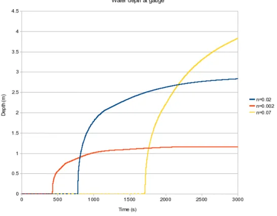
Wa-ter was added into the domain close to the upstream boundary at a rate of 160m3s−1for a total simulation time of 3000 seconds. A gauge measuring depth (relative to topography)

was simulated in a central position as shown in figure 3.3.

Figure 3.3: Location of gauge in domain marked with black dot and ‘1’. There is no water in the domain at the time shown; the green colours correspond to ‘dry land’ and are not

shown on the colourbar.

The gauge recorded depth throughout the simulations, which were carried out for

three different values of Manning’s friction coefficient,nin the domain. The friction values used were n = 0.02, n = 0.002 and n = 0.07. The first of these values is a reasonable

(38)

possible values. For each case the friction coefficient was the same in the whole of the domain, i.e. the value ofnin the rest of the domain was the same as in the channel. The

results are shown in figure 3.4.

Figure 3.4: Water depth at gauge with time for different channel friction parameters

Figure 3.4 shows that the channel friction parameter influences both the time taken to reach equilibrium, and the equilibrium depth in the channel, where the channel is defined

as the central 5 grid cells in thex direction for all y. The final water levels (after 3000 seconds) are shown in plan view for the three different values ofnin figure 3.5. The edges

of the channel are shown by the thin red lines and we can see in figure 3.5c that in the case in whichn= 0.07, some flooding of the domain took place (wherex >3000m). This

is because under these conditions water travels so slowly in the channel in thexdirection that it is forced out onto the banks. In all of the cases shown here the Manning’s friction

coefficient on the flood plain was the same as in the channel; making these values different will clearly affect the evolution of any inundation event.

(39)

(a)n= 0.002 (b)n= 0.02

(c)n= 0.07

Figure 3.5: Water depth in the domain at the end of the simulation for three different values of nin the channel. The domain is shown in plan view. Note the different scales

for the colourbars.

3.2.2 Slope at downstream boundary

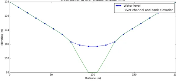
The effect of changing the parameter controlling the bathymetry slope at the down-stream boundary can be seen in the following simulations. In each case, a symmetrical

domain with a central channel was initially filled with water to a depth of approximately 4 m as shown in cross section in figure 3.6. The domain has a slope of 0.09% which caused

(40)

downstream end. No extra water was added to the domain during the simulations, which ran for 1500 seconds. Some water remained in the domain at the end of the simulations.

For one case the downstream slope was extrapolated into the ghost cells, and for the other case the ‘no slope’ condition was used, where the elevation in each ghost cells is set to be

the same as the domain cell next to it on the inside of the boundary.

Figure 3.6: Cross section of the domain, showing the channel filled with water at the start of the simulations. The green line shows the elevation of the domain and the blue points

show the water depth.

At the end of the simulations, the water profile is different for the two cases as shown

in figure 3.7. For the extrapolated boundary slope condition, the water is able to leave the domain cleanly; the flow over the boundary is the same as elsewhere in the domain.

For the no slope condition, water cannot leave the domain as fast and therefore builds up at the boundary.

(41)

(a) Extrapolated slope; water levels relative to topography in 3D

(b) No slope; water levels relative to topography in 3D

(c) Extrapolated slope; water levels relative to topography in plan view

(d) No slope; water levels relative to topography in plan view

Figure 3.7: Water profiles for the slope and no slope boundary conditions after 1500s.

3.3 Chapter summary

In this chapter we have described the inundation model used for the simulations in

chapters 4, 5 and 6 of this thesis. We have described the boundary condition options in Clawpack; our description of the treatment of source terms is presented as part of our paper Cooper et al. [2018b], reproduced in this thesis as chapter 4 (see section 4.8

for treatment of source terms). In this chapter we have also presented results of studies investigating the sensitivity of modelled water levels to the domain friction parameter and