Author(s)
Morino, Kai; Hirata, Yoshito; Tomioka, Ryota; Kashima,
Hisashi; Yamanishi, Kenji; Hayashi, Norihiro; Egawa, Shin;
Aihara, Kazuyuki
Citation
Scientific Reports (2015), 5
Issue Date
2015-05-20
URL
http://hdl.handle.net/2433/216227
Right
This work is licensed under a Creative Commons Attribution
4.0 International License. The images or other third party
material in this article are included in the article's Creative
Commons license, unless indicated otherwise in the credit line;
if the material is not included under the Creative Commons
license, users will need to obtain permission from the license
holder to reproduce the material. To view a copy of this
license, visit http://creativecommons.org/licenses/by/4.0/
Type
Journal Article
Textversion
publisher
Predicting disease progression from short
biomarker series using expert advice
algorithm
Kai Morino1, Yoshito Hirata1,2, Ryota Tomioka3, Hisashi Kashima4, Kenji Yamanishi1,5, Norihiro Hayashi6,
Shin Egawa6& Kazuyuki Aihara1,2
1Graduate School of Information Science and Technology, The University of Tokyo, Tokyo 113-8656, Japan,2Institute of Industrial
Science, The University of Tokyo, Tokyo 153-8505, Japan,3Toyota Technological Institute at Chicago, Chicago, Illinois 60637,
USA,4Graduate School of Informatics, Kyoto University, Kyoto 606-8501, Japan,5CREST, JST, Honcho, Kawaguchi, Saitama
332-0012, Japan,6Department of Urology, Jikei University School of Medicine, Tokyo 105-8461, Japan.
Well-trained clinicians may be able to provide diagnosis and prognosis from very short biomarker series using information and experience gained from previous patients. Although mathematical methods can potentially help clinicians to predict the progression of diseases, there is no method so far that estimates the patient state from very short time-series of a biomarker for making diagnosis and/or prognosis by employing the information of previous patients. Here, we propose a mathematical framework for integrating other patients’ datasets to infer and predict the state of the disease in the current patient based on their short history. We extend a machine-learning framework of ‘‘prediction with expert advice’’ to deal with unstable dynamics. We construct this mathematical framework by combining expert advice with a mathematical model of prostate cancer. Our model predicted well the individual biomarker series of patients with prostate cancer that are used as clinical samples.
M
athematical models of diseases have been constructed to understand the mechanisms of diseases1–7, provide diagnosis and prognosis8–10, and determine treatment options11–14. When we focus on a clinical setting, it is crucial that we can estimate the state of a disease from short biomarker observations. Clinicians make such estimations using their experience with previous patients (see Fig. 1a). To the best of our knowledge, such estimations have not been realized mathematically thus far. If such mathematical estimation is possible, then we can optimize a treatment option in a personalized way. The difficulty of estimations stems not only from a lack of information, but also the instability of biomarkers’ time-series, such as those for cancer volumes. Thus, our goal is to infer the state of a disease from both short, unstable time-series data of biomarkers obtained from a target patient and longer time-series data of biomarkers from previous patients who suffered from the same disease. We adopt the machine-learning framework of ‘‘online prediction’’, which integrates ‘‘experts’ advice’’15to make accurate predictions, where experts are short-term patterns of previous patients’ histories, which are conformed to the target patient time-series.A series of samples from a patient contains information on (often unstable) disease dynamics8,10such as rapid increase. By considering the time series observed from the unstable dynamics, we may be able to better under-stand the current disease state. Employing past patients’ time-series as experts and the target patient’s time-series as observations, we can predict a time-series with the standardexpert advicemethod15. However, this cannot be used directly, because we must deal with the unstable dynamics in which the value of a biomarker increases rapidly. In this paper, we propose an approach that couples an existing machine-learning technique with the instability possessed by the temporal disease datasets. Our method is based on the standard expert advice15, but deals with the instability of the underlying dynamics8,10by integrating trajectories in a database with weights that increase exponentially in time.
Results
The proposed method: temporal expert advice (TEA).We extend the standard expert advice method15to one that emphasizes near-past information. Thistemporal expert advice, or the TEA algorithm, consists of three steps (see Fig. 1b–d). TEA uses a collection of time-series, which we call experts, and weights each expert based on its agreement with the target time-series. The algorithm outputs a prediction by combining these experts.
SUBJECT AREAS: MACHINE LEARNING TUMOUR BIOMARKERS APPLIED MATHEMATICS Received 24 September 2014 Accepted 6 February 2015 Published Correspondence and requests for materials should be addressed to K.M. ([email protected]) 2 May 20150
The first step constructs an expert of a target system. There are two options. The first option is to use long time-series observed in the past as they are. We construct experts by simply inserting previous parts of the time-series or the datasets of previous patients. Letxj,lbe thelth point of thejth time-series in a database (j51, 2, …,J,l51, 2, …,L) andfi,tbe theith expert’s advice at timet. NumbersJandLare the number of series and the number of points in each time-series, respectively; We assume that the lengths of the time-series are equal, but it is easy to extend to cases of different lengths. LetPbe the number of points related to each expert. Then, we can define an expertf(L2P11)(j21)1i,k5xj,i1k21fori51, 2, …,L2P11,k5 1, 2, …,P. The second option is roughly to fit a mathematical model that has a set of parameters to a very short time-series, obtain the initial conditions for each set of parameters, and prepare the set of experts with these parameters. The details of this second rough option are discussed after we introduce a mathematical model of prostate cancer in the later section.
In the second step, TEA weights the trajectoriesfi,tin the database to generate an appropriate weighting for the most current state. Letyk denote the observation at timek, and letl(
?
,?
) be a loss function. When we include the next point, the weightswi,tare updated accord-ing to a formula obtained by modifyaccord-ing the standard expert advice15. To achieve this, we sum the loss at each time step with a coefficient as follows: Li,t{1~ Xt{1 k~1ak(t)l fði,k,ykÞ, ð1Þ Lt{1~ Xt{1 k~1ak(t)l pð k,ykÞ: ð2Þ The modified form considers the instability of the underlying dynamics by introducing a coefficientak(t), which measures the reliability of the prediction at, and increases exponentially with, time ksuch thatak(t)5lk21orlkwithl.1. Thus, the real valuesLi,tandFigure 1|Schematic illustration of the estimation from short observations of biomarkers.(a) The prediction of clinicians. (b) The first step of TEA. (c) The second step of TEA. (d) The third step of TEA.
Ltare the exponentially weighted losses of theith expert and the predictor up to time t, respectively. We defineL0 5Li,050 for simplicity. The weight of the expert is updated as
wi,t{1~exp({gLi,t{1), ð3Þ wheregis a learning rate. Chernov and Zhdanov16proposed a modi-fied expert advice method in which they definedak(t)5rt2k21and 0,r,1. We call this the ‘‘CZ method’’.
The third step predicts future states of the target system by apply-ing the obtained weightapply-ing to the future trajectories in the database15. We can generate a point prediction by simply adding the qsteps ahead of the trajectories with the weights obtained in the second step as follows: ptzq{1~ PN i~1 wi,t{1fi,tzq{1 PN i~1 wi,t{1 , ð4Þ
whereNdenotes the total number of experts. We can also generate a distributional prediction by assuming the distribution of obser-vational errors, and summing this error distribution with the weights. To make these predictions online, we repeat the second and third steps iteratively.
Upper bound of the regret of TEA.We derive an upper bound of the regret of TEA. The primary property peculiar to TEA lies in our definition of ak(t). We define the coefficient asak(t)5lk21 orlk, where l . 1. The choice of these two options depends on each situation. When a given data is too short, we choose the latter, e.g. our prediction about the biomarker of prostate cancer, or PSA (prostate-specific antigen). LetL^t andL
^
i,tbe the accumulated losses for the proposed method. We call these theexponential accumulated lossesto distinguish them from the standard accumulated losses. In addition, we define the regret as R^t~L
^
t{ min i~1,:::,NL
^
i,t. The upper bound of the regret withak(t)5lk21is then given by
R^tƒlnN g z e2g 8 :l2t{1 l2{1: ð5Þ
Proof of the upper bound in our proposed method.We give a proof of Eq. (5) in a similar way to the Proof of Theorem 2.2 in Ref. 15. Define a new variableWt:
XN k~1w ^ k,t~ XN k~1exp {gL ^ k,t . We will consider the upper and lower bounds of ln(Wt/W0) to construct the upper bound of the regret. First, we obtain the lower bound of ln(Wt/W0) as lnWt W0 ~lnWt{lnW0 ~ln XN k~1exp {gL ^ k,t {lnN §ln max k~1,:::,Nexp {gL^k,t {lnN ~{g min k~1,:::,NL ^ k,t{lnN: ð6Þ
Second, we derive the upper bound of ln(Wt/W0). Observe that L ^ k,t~L ^ k,t{1zlt {1l f k,t,yt
ð Þ. Then, we can reformulate ln(Wt/Wt21) as follows: ln Wt Wt{1 ~ln PN k~1exp({gL ^ k,t) PN k~1exp {gL ^ k,t{1 ~ ln PN k~1exp({gL ^ k,t{1)exp {glt {1l f k,t,yt ð Þ PN k~1exp {gL ^ k,t{1 : ð7Þ
Equation (7) can be regarded as the average of random variable exp(2glt21l(f
k,t,yt)) with a probability mass function proportional to exp({gL^k,t{1). Lemma 2.2 of Ref. 15 states that
lnEðexpð Þsx ÞƒsE xð Þzs 2ðb{aÞ2
8 : ð8Þ
Here, we assume thatxis a random variable satisfyinga#x#b, and that the inequality holds whensis any real number.
Replacesby2glt21andxbyl(f
k,t,yt). Then, the upper bound of Eq. (7) can be found using Eq. (8) as follows:
ln Wt Wt{1 ~lnEexp{glt{1l fðk,t,ytÞ ƒ{glt{1E l fððk,t,ytÞÞzg 2l2(t{1)e2 8 ~{glt{1 PN k~1exp {gL ^ k,t{1 l fðk,t,ytÞ PN k~1exp {gL ^ k,t{1 zg 2l2(t{1)e2 8 ƒ{glt{1l PN k~1exp {gL ^ k,t{1 fk,t PN k~1exp {gL ^ k,t{1 ,yt 0 B @ 1 C Azg 2l2(t{1)e2 8 ~{glt{1l PN k~1w ^ k,t{1fk,t PN k~1w ^ k,t{1 ,yt ! zg 2l2(t{1)e2 8 ~{glt{1l p^ t,yt zg 2l2(t{1)e2 8 : ð9Þ
We assume thatl(
?
,?
) is convex as described above. Then, the upper bound of ln(Wt/W0) can be derived aslnWt W0 ~Xt k~1ln Wk Wk{1 ƒ Xt k~1 {gl k{1l p^ k,yk zXt k~1 g2l2(k{1)e2 8 ~{gL^tzg 2e2 8 :l2t{1 l2{1: ð10Þ
Because Eqs. (6) and (10) provide lower and upper bounds of ln(Wt/ W0), respectively, the following inequality is obtained:
{g min k~1,:::,NL ^ k,t{lnNƒ{gL ^ tz g2e2 8 :l 2t{ 1 l2{1: ð11Þ By substituting the regret R^t~L
^
t{ min k~1,:::,NL
^
k,t into Eq. (11), we finally reach the following inequality:
R ^ tƒlnN g z ge2 8 :l2t{1 l2{1: ð12Þ (Proof end)
Optimization of the upper bound of TEA.We minimize the upper bound of Eq. (12) overg. First, we differentiate the upper bound with respect togas follows: {lnN g2 z e2 8 :l2t{1 l2{1 ~0: ð13Þ The solution is g~2 ffiffiffi 2 p e : ffiffiffiffiffiffiffiffiffiffiffiffiffiffiffiffiffiffiffiffiffiffiffi l2{1 l2t{1 :lnN s , ð14Þ
which gives the smallest upper bound. Replacinggin the upper bound ofR^twithg*, we obtain the following optimal upper boundA
^ (t): A^(t)~ effiffiffi 2 p : ffiffiffiffiffiffiffiffiffiffiffiffiffiffiffiffiffiffiffiffiffiffiffi l2t{1 l2{1 :lnN s : ð15Þ
Although this optimal upper bound perhaps seems to be curious at a glance due to its exponential increase witht, this is caused by the definition of the accumulated losses Eqs. (1) and (2) with ak(t)5
lk21
.This regret can be compared with the normal types of regrets using relationship described in the next section. Whene51 andlR 1, the optimal upper boundA^(t)coincides withpffiffiffiffiffiffiffiffiffiffiffiffiffiffiffiffitlnN=2, which is the upper bound obtained in the standard expert advice method15.
Comparison between the proposed method and the Chernov– Zhdanov method. Here, we highlight the difference between the CZ method and the proposed TEA method. The first point of difference is the optimal upper bound of the regret. We briefly introduce the optimal upper bound of the CZ method16. LetL^
i,tand
^
Ltbe the accumulated losses for theith expert and the predictor for the CZ method, respectively. Then, the optimal upper boundA^c(t)of the regretR^t~^Lt{ min
i~1,:::,N
^
Li,tfor the CZ method is given by
^ Ac(t)~e ffiffiffiffiffiffiffiffiffiffiffiffiffiffiffiffiffiffiffiffiffiffi 1{rt 1{r:lnN s : ð16Þ
Note that we assume the case where the value of the decay raterdoes not depend ontork. See Ref. 16 for the proof.
Although we cannot directly compare these regrets, we can compare them after normalization. Assuming that the decay rates are equal, namelyl5r21, the regretsR^
tand^Rthave the following relation:
^ Rt~ Xt k~1r t{k l ^p k,yk { min i~1,:::,Nl fði,k,ykÞ ~rt{1Xt k~1l k{1 l ^pk,yk { min i~1,:::,Nl fði,k,ykÞ ~rt{1R^ t: ð17Þ
Using this relation, a comparison between the two upper bounds is feasible. Multiplying the optimal upper boundA^(t)byrt21, we obtain the normalized optimal upper boundA^m(t)as
A^m(t)~rt{1A^(t) ~rt{1 effiffiffi 2 p : ffiffiffiffiffiffiffiffiffiffiffiffiffiffiffiffiffiffiffiffiffiffiffiffiffiffiffi 1{r{2t 1{r{2:lnN s ~e ffiffiffiffiffiffiffiffiffiffiffiffiffiffiffiffiffiffiffiffiffiffiffiffi 1{r2t 1{r2: lnN 2 s : ð18Þ
Then, the following relation is obtained: A^m(t) ^ Ac(t) ~ ffiffiffiffiffiffiffiffiffiffiffiffiffiffiffiffiffi 1 2 :1zrt 1zr s v1: ð19Þ This result means that the normalized optimal upper bound of the proposed method is always smaller than that of the CZ method when 0,r,1.
Next, we compare the weights produced by the two methods. Let ^
wi,tandw
^
i,tbe the weights of theith expert at timetin the CZ and TEA methods, respectively. Similarly to the derivation of Eq. (17), the accumulated losses of both methods are related by^Li,t~rt
{1L^
i,t. Substituting this relation intow^
i,t, we have w^i,t~exp {gL ^ i,t ~exp{g^Li,t:r{tz1 ~exp{g^Li,tr {tz1 ~ðw^i,tÞr{tz1: ð20Þ
Equality (20) means that the proposed TEA method tends to assign reliable experts with heavier weights than the CZ method. This implies thatw^i,t .XN j~1w ^ j,t§w^i,t.X N
j~1w^j,t for reliable experts becauser2t11$1.
Examples of time-series prediction for mathematical models.We demonstrate the superiority of the TEA method to both the CZ method and the standard expert advice in online time-series prediction using toy examples. We use the He´non map17and the Ikeda map18 for our demonstration. These two models are commonly used to test nonlinear time-series analysis methods, which exhibit typical unstable chaotic dynamics. First, we generate time-series for the database using various values of parameters. We then generate a target time-series for prediction using a set of parameter values that is different from those used to generate the database. We prepareM3Sexperts for the database, whereMis the number of parameter sets. For each parameter set, we generateS experts with different initial conditions. In numerical simulations of TEA, we sete 51 andg~
ffiffiffiffiffiffiffiffiffiffiffiffiffiffiffiffiffiffiffiffiffiffiffiffiffiffiffiffiffi 8:l 2{1 l8{1 :lnMS s . We also setl5 r21andr50.9. See Algorithm 2 in Ref. 16 for the implementation of the CZ method, and Ref. 15 for that of the standard expert advice.
The He´non map17is a two-dimensional map defined as xnz1~1{ax2nzyn,
ynz1~bxn:
ð21Þ
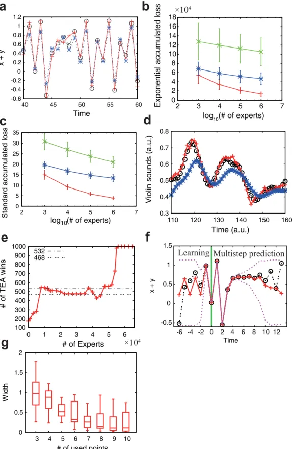
We set the parameters ata51.35 andb50.15 to generate the target time-series. Note that the dynamics produced by this parameter set is of deterministic chaos. The experts’ parameters are uniformly chosen fromag[1.3,1.4] andbg[0.1,0.2]. The initial conditionsx0andy0 are randomly chosen in [20.02, 0.02]3[20.02, 0.02], and the map is iterated for 1,000 steps to eliminate transient effects. We assume that we observe and predict the value ofx1y. We use this assump-tion because we can observe a scalar biomarker of PSA in the prostate cancer application discussed later. The results presented in Figs. 2a, 2b, and 2c show that the proposed TEA achieves better online time-series prediction than the standard expert advice and the CZ method. We chooseM5100 andS51,000 in Figs. 2a, 2f, and 2g. Another example of the Ikeda map is shown in Supplementary Fig. S1 (see also Supplementary Information).
The proposed TEA method provides the best online prediction in different toy examples. The more experts we use, the smaller the prediction errors become. When a large number of experts are used, the proposed TEA tends to achieve the best online time-series pre-diction. We need to decay the past information in these examples, because the unstable chaotic dynamics rapidly loses the memories.
Examples of time-series prediction for real datasets. We now consider two real datasets: violin sounds19and the membrane potential of squid giant axons20. The violin sounds are RWC-MDB-I-2001 No. 15 in the RWC Music Database (Musical Instrument Sound). Previous studies on squid giant axons have demonstrated the chaotic nature of the underlying dynamics20–23. These time-series are both scalar and real-valued. We divide each time series into two. The first part is used to build the database, and the second constructs the targets for online prediction. We use M 5 1,000 and M 5 120 targets for the analysis of violin sounds and squid giant axon data, respectively. The lengths of the target data are 311 for the violin data and 51 for the squid giant axon data; numbers and lengths of target data are determined by the lengths of the original datasets.
We compare five methods using these real data. These are our TEA method, the CZ method, the standard expert advice, the persistence prediction, and the average prediction. The persistence prediction is a method that we let the current value to be the prediction for the next time point. We compare each pair of the method individually, and count the number of points at which the prediction by one method is better than the other for each target time-series. If one method is superior at more than half the data points, we declare that method the winner on the target data. We exclude the initial ten points from the analysis, because we cannot prepare the learning part. Finally, we count the number of wins and losses for each pair among the five methods. In the TEA numerical simulations, we set e 5 1 and
g~ ffiffiffiffiffiffiffiffiffiffiffiffiffiffiffiffiffiffiffiffiffiffiffiffiffiffiffi 8:l 2{1 l8{1 :lnM s
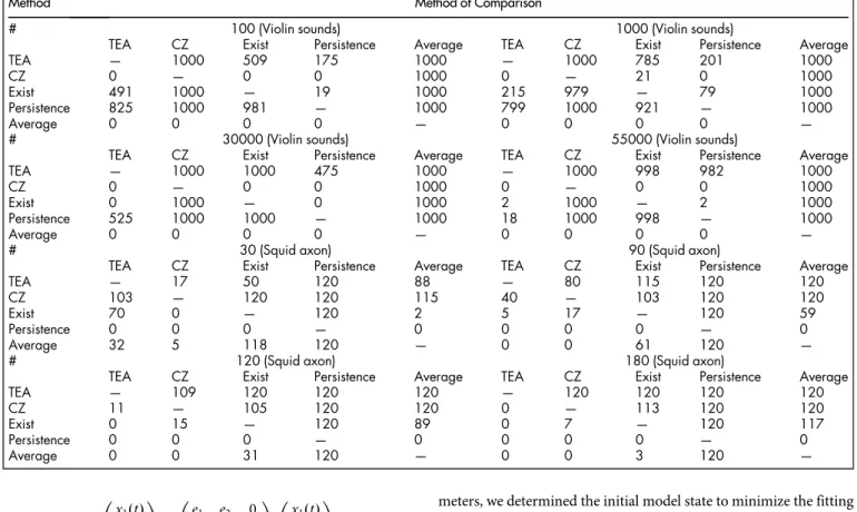
. We also setl5r21andr50.9. The violin sound19results are shown in Figs. 2d and 2e, and Tables 1. For this dataset, our method and the persistence prediction produce much better results than the other methods. Therefore, we next compare our TEA method with the persistence prediction with respect to the number of experts. We use the binominal test for the analysis, i.e., if the number of wins is greater (smaller) than 531 (469), the method is significantly superior (inferior) to the other method with respect to the 95% confidence level two-sided binominal test. When the num-ber of experts is large, our TEA method is significantly superior to the persistence prediction, as shown in Fig. 2e and Table 1. In the example of squid giant axon20, the proposed TEA is also better than the other four methods when the number of experts is large, espe-cially when greater than or equal to 87, as shown in Fig. 3 and Table 1. In conclusion, our TEA method tends to provide the best predic-tion when the number of experts is large. The precise number of experts for which this is the case may change depending on the given data, the length of targets, and the decay parameter.
Distribution prediction to the mathematical models.We applied the distribution prediction to time-series of the He´non map. The distribution prediction will be explained in the later Method section. The setup is similar to that for the point prediction, except that we provide the prediction as a distribution. The results are presented in Figs. 2f and 2g. The width of the distribution prediction is narrow immediately after the learning period (Fig. 2f), then grows gradually as the number of prediction steps increases because of the instability of the underlying dynamics. The predicted confidence interval tends to contain the actual values. When we increase the number of points used for prediction, the width of the distribution prediction becomes narrower (Fig. 2g). We use values ofS51,000 and M5100 in Figs. 2f and 2g. In the TEA numerical simulations, we set
e51 andg~1 l ffiffiffiffiffiffiffiffiffiffiffiffiffiffiffiffiffiffiffiffiffiffiffiffiffiffiffiffiffi 8:l 2{1 l8{1 :lnMS s
. The number of trials is 40 in each box in Fig. 2g. Restricting the range oflto 1,l,2 gives a better prediction. We generate the target and experts’ time-series as in the previous section. We also obtain the distribution prediction of the Ikeda map usingS51,000 andM5100, as shown in Fig. S1f. The result is very similar to that of the He´non map. Again, restricting the range oflto 1,l,2 gives a better prediction.
Mathematical models of prostate cancer.TEA can be applied to clinical problems, such as the prediction of prostate-specific antigen (PSA) after some initial treatments, while waiting to start an additional treatment. We apply TEA to the prediction of tumor markers for prostate cancer PSA. Before the technical details, we introduce a mathematical model of prostate cancers in this section.
Patients had already received radical prostatectomy as an initial treatment. Then, clinicians followed postoperative PSA levels to determine when to commence salvage treatment. Although the tim-ing at which patients start salvage treatment is an important prob-lem, there is no definitive agreement on when this to be started. Currently, clinicians are determining the start of salvage treatment based on their discretion. The clinical part of this study was approved by the ethics committees of Jikei University School of Medicine and The University of Tokyo. All patients provided written informed consent. Cancer cells tend to thrive under an androgen-rich envir-onment. Meanwhile, lowering androgen levels makes cancer cells grow slowly or rather decline. Because of this characteristics, clin-icians suppress the androgen concentration with hormone therapy. However, when cancer cells remain exposed to an androgen-poor environment, they often acquire the ability to grow without andro-gen. This growth signals a cancer relapse. Intermittent androgen suppression was proposed to delay the relapse of cancer24. In inter-mittent androgen suppression, we start hormone therapy, but stop when PSA levels have decreased sufficiently. Then, we wait until PSA increases and reaches a threshold value. After reaching this thresh-old, we resume hormone therapy. We repeat this process to delay the relapse. However, clinical trials show that the effects of intermit-tent androgen suppression depend on individual patients, and are limited25,26.
Here, we use a mathematical model8of intermittent androgen sup-pression for prostate cancer24–26. This model was constructed based on data of Canadian patients25,26whose PSA had increased to some extent after radiation therapy, and were later treated by intermittent andro-gen suppression. Because the model of Ref. 8 has a small number of parameters, it is reasonable to predict the future PSA values with this simple model and very short time-series, although several mathemat-ical models have been proposed to describe dynamics under intermit-tent androgen suppression4–6,8,10,27–31. In the model described in Ref. 8, we assume that there are three classes of cancer cells: androgen dependent cancer cellsx1, androgen independent cancer cells gener-ated through reversible changesx2, and androgen independent cancer cells generated through irreversible changesx3. When the hormone therapy is underway,x1may change tox2orx3. When the hormone therapy is stopped,x2may return tox1, whereasx3cannot return tox1 orx2because of genetic mutation. We previously verified two import-ant properties of this model: namely, a piecewise linear model is sufficient to describe the dynamics of PSA, and the androgen concen-tration need not be explicitly included in the model8. Based on these verified properties, we can simply construct the mathematical model as d dt x1(t) x2(t) x3(t) 0 B @ 1 C A~ d1 0 0 d2 d3 0 d4 d5 d6 0 B @ 1 C A x1(t) x2(t) x3(t) 0 B @ 1 C A, ð22Þ
Figure 2|Examples of prediction by TEA.(a) Online point prediction of the He´non map. (b, c) The number of experts versus the exponential accumulated loss of errors and the standard accumulated loss of errors in the prediction of the He´non map. (d) Online point prediction of violin sounds. (e) The number of experts versus the number of wins out of 1,000 online prediction trials against the persistence prediction in the violin example. (f) Distribution prediction of the He´non map. (g) Confidence interval width against the number of used points shown in box plots. In panels (a) and (f), actual observations are shown with black#and dotted lines, TEA predictions are shown with red1and solid lines, and the prediction given by the method of Chernov and Zhdanov is shown with blue*and dashed lines. In panel (f), the purple dotted lines show the 95% confidence interval of the distribution prediction, and the green line divides the learning period and the multistep prediction period. In panels (b) and (c), red, blue, and green error bars correspond to TEA, the method of Chernov and Zhdanov, and the standard expert advice, respectively. In panel (e), the dotted lines show the 95% confidence interval under the null-hypothesis of even chance.
d dt x1(t) x2(t) x3(t) 0 B @ 1 C A~ e1 e2 0 0 e3 0 0 0 e4 0 B @ 1 C A x1(t) x2(t) x3(t) 0 B @ 1 C A, ð23Þ
for the off-treatment period8. Here,d
1,d2,d3,d4,d5,d6,e1,e2,e3, ande4 are model parameters. We assume that a PSA measurement is repre-sented byx11x21x3for simplicity. Thus, we must specify these 10 parameters for the dynamics and three other parameters for the initial conditions of x1,x2, and x3. If we try to find these 13 parameters directly only from a single target patient, we would need to obtain a long time-series. The application of the proposed TEA algorithm makes the required observation period of PSA measurements shorter by integrating observations from the target patient with the long time-series data of PSA measurements obtained from previous prostate cancer patients. We note that we only analyze the off-treatment period in this paper, because the target dataset is about the follow-up period after an initial treatment. Therefore, we need 4 control parameters and initial conditions.
Construction of experts for prediction of PSA for prostate cancer. In this paper, we have two datasets; one is a dataset of Canadian patients with many data points; the other is a dataset of Japanese patients with short time points. We need a long time-series to efficiently estimate model parameters. Therefore, we select Canadian datasets for estimation of parameters and Japanese datasets for predicting targets.
In applying TEA to prostate cancer, we first prepared 72 sets of model parameters, each of which was obtained from one of 72 Canadian prostate cancer patients treated with intermittent andro-gen suppression. These parameters were obtained from Ref. 8. We note that our prediction target dataset corresponds to the off-treat-ment period in the model8. Second, we chose the number of obser-vation points to use as known data points. This must be at least three because of the model dimensions8. Third, using each set of
para-meters, we determined the initial model state to minimize the fitting error between the initial three or more PSA measurements and the model output. The optimal initial conditions were selected by min-imizing the following cost function:
XK k~1 X3 j~1xj(tk){y tð Þk z X3 j~1h xjð Þtk , ð24Þ
whereh(x)51015(12x) forx,0 andh(x)50 forx$0, wheret kis the kth observation time. We denote the number of observation points used for learning byK. The method of obtaining the initial conditions was similar to that in Ref. 8. Fourth, we ran the model with each set of parameters and the corresponding initial conditions to construct the database of expertsfi,t; thus, we have 72 experts.
Estimation of learning parameters.We applied the second step of the TEA algorithm to determine the weights of the PSA measure-ments. Then, we applied the third step of the TEA algorithm to obtain the distribution prediction. We determined the optimal decay rate l by minimizing the error between the last learning observation and the prediction. We restricted the range oflto 1, l , 2 to obtain better predictions. The standard deviation s is estimated as follows. We ran the distribution prediction with the obtained initial conditions and the decay parameter. We set the standard deviationsto the mean of the absolute errors between the median of the distribution prediction and the corresponding observation when the mean is taken during the learning period.
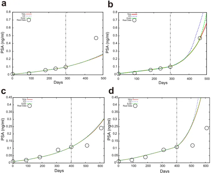
Application of TEA to prediction of PSA for prostate cancer.We predict the values of PSA with distribution prediction. The distribution prediction of PSA with TEA is shown in Fig. 4. Here we evaluate the larger side of the predicted distribution, because overlooking high PSA is highly undesirable in a real clinical setting. We show seven pointsut(Q) of the predicted distribution (97.5%, 87.5%, 75%, 65%, 60%, 55%, and 52.5%) in these figures, whereut(Q) is defined as
Table 1 | Analysis of violin sounds and the membrane potential of squid giant axon. The number of wins between each pair of the five prediction methods is shown. The each number indicates the number of experts in each case.
Method Method of Comparison
# 100 (Violin sounds) 1000 (Violin sounds)
TEA CZ Exist Persistence Average TEA CZ Exist Persistence Average
TEA — 1000 509 175 1000 — 1000 785 201 1000
CZ 0 — 0 0 1000 0 — 21 0 1000
Exist 491 1000 — 19 1000 215 979 — 79 1000
Persistence 825 1000 981 — 1000 799 1000 921 — 1000
Average 0 0 0 0 — 0 0 0 0 —
# 30000 (Violin sounds) 55000 (Violin sounds)
TEA CZ Exist Persistence Average TEA CZ Exist Persistence Average
TEA — 1000 1000 475 1000 — 1000 998 982 1000
CZ 0 — 0 0 1000 0 — 0 0 1000
Exist 0 1000 — 0 1000 2 1000 — 2 1000
Persistence 525 1000 1000 — 1000 18 1000 998 — 1000
Average 0 0 0 0 — 0 0 0 0 —
# 30 (Squid axon) 90 (Squid axon)
TEA CZ Exist Persistence Average TEA CZ Exist Persistence Average
TEA — 17 50 120 88 — 80 115 120 120
CZ 103 — 120 120 115 40 — 103 120 120
Exist 70 0 — 120 2 5 17 — 120 59
Persistence 0 0 0 — 0 0 0 0 — 0
Average 32 5 118 120 — 0 0 61 120 —
# 120 (Squid axon) 180 (Squid axon)
TEA CZ Exist Persistence Average TEA CZ Exist Persistence Average
TEA — 109 120 120 120 — 120 120 120 120
CZ 11 — 105 120 120 0 — 113 120 120
Exist 0 15 — 120 89 0 7 — 120 117
Persistence 0 0 0 — 0 0 0 0 — 0
ðut(Q)
0 p ^
t(x)dx~Q: ð25Þ
Note thatQis the intended value of the probability, i.e. 0.975, 0.875, 0.75, 0.65, 0.6, 0.55, and 0.525, respectively, in this situation. We obtained the proportion of PSA values that are less than the intended probability for eachQ, and counted the PSA data points that are next to the final data points in the learning period; namely, if we are using three data points for learning, we count the fourth data point. In this paper, we focus on the predictability of the next point. The results are summarized in Table 2. Note that TEA can predict not
only the next data point, but also those far in the future. We predicted the future PSA values for 88, 86, 80, and 69 patients when we used the first three, four, five and six time points, respectively. We also conducted numerical simulations using CZ and the standard expert advice. The predicted distributions were different for each method, as shown in Fig. 5. In numerical simulations, we sete5 1. We arrange the learning rate as four constant values g~1 l ffiffiffiffiffiffiffiffiffiffiffiffiffiffiffiffiffiffiffiffiffiffiffiffiffiffi 81{l 2 1{l2vlnM s
with v 5 1, 2, 3, and 4. In addition, we increasevas the number of the learning points increases. We note thatM572 is the number of experts. We also arrange the learning Figure 3|Online time-series prediction of membrane potential of squid giant axon.The decay parameter was fixed atr50.9. (a, b, c) The observed time-series is represented by black lines. The number of experts is 160. The predicted time-series represented by a red dashed line in (a), a blue dashed line in (b), and a green dashed line in (c) are obtained by our method, CZ, and the standard expert advice, respectively. (d) The number of times our method outperforms CZ (blue*), the standard expert advice (green3), and the average prediction (purple%) (out of 120) are shown. When the number of wins for a method is greater than 71 (the dashed-dotted horizontal line), it is significantly better than the other method in terms of the binominal test. When it is smaller than 49 (the double-dotted line), the opposite is true. (e) The number of times the CZ method outperforms our method (red1), the standard expert advice (green3), and the average prediction (purple%). (f) The number of times the standard expert advice outperforms our method (red1), CZ (blue*), and the average prediction (purple%).
rate as g~ ffiffiffiffiffiffiffiffiffiffiffiffiffi
8lnM v
r
for the standard expert advice and g~2
ffiffiffiffiffiffiffiffiffiffiffiffiffiffiffiffiffiffiffiffiffiffi
1{r 1{rvlnM
r
for the CZ method.
TEA exhibits the best performance among the three methods, because each proportion tends to be closest to the specified value ofQ. These results imply that our proposed prediction method may be reasonable for real applications in a clinical setting. We also checked the prediction performance in terms of the median using the mean absolute error (MAE) as summarized in Supplementary Table S1. As a result, TEA shows the best performance in the mean-ing of the average MAE among the four cases. We note that the CZ method showed good performance in terms of the root mean square error (RMSE), however, we believe that the MAE suits our situation because we employed the absolute error function for the learning period.
Discussion
In general, clinicians provide a salvage treatment with patients who had recurrence after surgery. Although many studies show the clin-ical benefit of a salvage treatment for patients with prostate cancer, current studies have reported that an earlier salvage treatment, espe-cially for local recurrence, could improve clinical outcomes32. These results suggest that post-operative patients with lower PSA values may have a higher frequency of local recurrence that could be effi-ciently treated by radiotherapy. If clinicians can accurately assess the
PSA failure at an earlier stage than the present standard criterion of PSA failure which is that the PSA value increases to 0.2 (ng/ml) or more after surgery, salvage treatments could be more effectively scheduled for each patient, improving the final clinical outcome33. However, there is still no standardized criterion to determine the best timing of salvage treatments32,33. Combined with a mathematical model8, TEA or its further extensions may be able to potentially predict the PSA dynamics in patients before PSA failure. Therefore, the proposed TEA could become the basis of a new standard index for earlier prediction of PSA failure using a simple mathematical solu-tion, that offers important information for a suitable salvage treat-ment after surgery7,34,35.
The more experts we use, the more (numerically) accurate the prediction tends to become (Figs. 2b, 2c, and 2e); in this sense, the accumulation of datasets is important. Additionally, the longer the learning period, the more accurate the TEA prediction tends to become in the toy examples (Fig. 2g). This could be because the toy examples have bounded unstable dynamics. The prediction error does not monotonically decrease with an increase of the learning data points in the example of prostate cancer (Tables 2 and S1), because PSA tends to increase monotonously in time. TEA exhibits the best performance in our analyses. The proposed combination of the expert advice with a predicted distribution enhances the reliability of prediction. This is important in many applications, and especially in medicine.
In summary, we have demonstrated that TEA can infer the state of a target system, by combining its short time-series and the expert Figure 4|Results of the distribution prediction of PSA in a patient.The black#shows the actual PSA observations. We used the (a) first three, (b) four, (c) five, and (d) six observation points to predict the next data points for the patient with the TEA(v51). The red curve shows the median distribution prediction. Other dotted lines indicate as denoted in each figure. The same patient data are used in all the figures.
advice constructed as a collection of longer time-series. The proposed TEA may be applied to any problems where a short time-series and its database are given, as demonstrated in the violin and squid giant axon examples, although we primarily intend to apply TEA in clin-ical settings, such as inferring the state of a disease using a short time-series from the target patient and longer time-time-series from previous patients with the same disease. We hope that TEA improves the overall survival and/or quality of life for patients.
Methods
Standard expert advice method.The expert advice method15is an online predictor in machine learning. We briefly introduce the standard expert advice method in this section. See the book of Cesa-Bianchi and Lugosi15for a more detailed introduction. The expert advice consists of experts and a predictor. At each time step, each expert gives the prediction on the future. The predictor makes a prediction for the future by weighting these pieces of advice based on the experts’ prediction history. After a new outcome is observed, the predictor updates the experts’ weights using the losses produced in the current step. We iterate these steps to realize online prediction. Letfi,t
be theith expert’s advice at timetandNbe the number of experts. We assign each expert the weightwi,tat timet, and obtain the prediction by averaging the experts’
advice as pt~ PN i~1wi,t{1fi,t PN i~1wi,t{1 , ð26Þ wi,t~expð{gLi,tÞ, ð27Þ
whereptis the prediction at timet,gis a constant, andLi,tis the accumulated loss for
theith expert at timet. Better experts have smaller accumulated losses, and hence have larger weights. The accumulated losses for theith expert and the predictor at timetare Li,t~ Xt k~1l fði,k,ykÞ, ð28Þ Lt~ Xt k~1l pð k,ykÞ, ð29Þ
whereykis the observation at timek, andl(x,y) is a convex loss function, typically the
absolute errorjx2yjor squared error (x2y)2. We evaluate the performance of the predictor by a regret, which is defined as the predictor’s accumulated loss minus the accumulated loss for the best expert. Mathematically, the regretRtis defined as
Rt:Lt{ min i~1,:::,NLi,t ƒlnN g z e2g 8 t, ð30Þ
whereeis the maximum value ofjl(?,?)j. Namely, the regret is bounded above by the right-hand side of Eq. (30) (see Ref. 15 for the derivation). We obtain the following optimal constantg*by minimizing the upper bound overg:
g~ 1 e ffiffiffiffiffiffiffiffiffiffiffiffiffiffi 8 lnN= t q : ð31Þ
When replacinggwithg*, we obtain the optimal upper bound of the regretRtas
epffiffiffiffiffiffiffiffiffiffiffiffiffiffiffiffitlnN=2. We call the accumulated losses defined in Eqs. (28) and (29) thestandard accumulated losses.
Although the standard expert advice can be applied in many cases, the method is not suited to the prediction of unstable systems, in which the recent history should be emphasized to predict the future more accurately. Thus, we extended the standard expert advice by placing greater weights on recent past information. We call our extension the temporal expert advice, or TEA.
Distribution prediction.Here, we extend the TEA method for point prediction to the prediction of distribution, so that we can handle the prediction of biomarkers. For this purpose, we introduce the distribution prediction of theith expert at timet p^i,t(x)as
follows: p ^ i,t(x)~ 1 ffiffiffiffiffi 2p p sexp {ðx{fi,tÞ 2 2s2 , ð32Þ
wheresis the standard deviation. This distribution is given under the assumption that a point predictionfi,tis disturbed by various errors and that the error is normally
Table 2 | Prediction results for real PSA datasets. The proportions of PSA data points that are followed by the TEA, CZ, and Existing prediction are shown againstQ%, points of the predicted distribution from below. A learning rategis changed withv. An abbreviation t.v. indicates time-varying. We consider data points that are next to the final point used for the learning period. We underline the best method in each case.
CIQ Used points TEA CZ Exist t.v. v51 2 3 4 t.v. 1 2 3 4 t.v. 1 2 3 4 97.5 3 100 100 100 100 100 100 100 100 100 100 100 100 100 100 100 4 100 98.8 100 100 100 100 100 100 100 100 100 100 100 100 100 5 100 100 100 100 100 100 100 100 100 100 100 100 100 100 100 6 100 92.8 100 100 100 100 100 100 100 100 100 100 100 100 100 87.5 3 89.8 92 90.9 89.8 89.8 89.8 89.8 89.8 89.8 89.8 89.8 92 89.8 89.8 89.8 4 93 94.2 94.2 93 93 93 93 94.2 93 93 93 94.2 94.2 93 93 5 98.8 96.2 97.5 98.8 96.2 98.8 98.8 98.8 98.8 98.8 98.8 97.5 97.5 98.8 98.8 6 98.6 87 91.3 97.1 97.1 98.6 98.6 98.6 98.6 98.6 98.6 95.7 95.7 97.1 97.1 75 3 75 75 75 75 75 75 75 75 75 75 75 75 75 75 75 4 84.9 84.9 84.9 84.9 84.9 84.9 84.9 84.9 84.9 84.9 84.9 84.9 84.9 84.9 84.9 5 91.2 87.5 90 90 90 91.2 91.2 91.2 91.2 91.2 90 90 90 90 90 6 89.9 75.4 78.3 84.1 85.5 91.3 89.9 89.9 89.9 91.3 87 87 87 87 87 65 3 69.3 69.3 69.3 69.3 69.3 69.3 69.3 69.3 69.3 69.3 69.3 69.3 69.3 69.3 69.3 4 79.1 80.2 80.2 80.2 80.2 79.1 79.1 79.1 79.1 79.1 80.2 80.2 80.2 80.2 80.2 5 88.8 82.5 87.5 88.8 88.8 88.8 88.8 88.8 88.8 88.8 88.8 87.5 87.5 88.8 88.8 6 84.1 72.5 72.5 76.8 78.3 82.6 82.6 84.1 84.1 84.1 84.1 78.3 79.7 81.2 81.2 60 3 67 68.2 68.2 67 67 67 67 67 67 67 67 68.2 67 67 67 4 79.1 77.9 79.1 79.1 80.2 77.9 77.9 77.9 77.9 77.9 80.2 79.1 79.1 79.1 79.1 5 85 81.2 83.8 85 85 86.2 85 85 86.2 86.2 85 83.8 85 85 85 6 78.3 71 72.5 75.4 76.8 79.7 78.3 78.3 79.7 79.7 78.3 75.4 76.8 78.3 78.3 55 3 65.9 64.8 64.8 64.8 65.9 65.9 65.9 65.9 65.9 65.9 65.9 64.8 64.8 64.8 65.9 4 73.3 73.3 73.3 73.3 74.4 73.3 74.4 73.3 73.3 73.3 73.3 74.4 74.4 74.4 74.4 5 82.5 78.8 78.8 82.5 82.5 81.2 82.5 82.5 82.5 82.5 82.5 81.2 81.2 82.5 82.5 6 75.4 71 72.5 72.5 73.9 76.8 72.5 73.9 73.9 75.4 75.4 75.4 73.9 73.9 73.9 52.5 3 64.8 64.8 64.8 64.8 64.8 64.8 64.8 64.8 64.8 64.8 64.8 64.8 64.8 64.8 64.8 4 70.9 73.3 72.1 70.9 69.8 70.9 70.9 70.9 70.9 70.9 72.1 74.4 73.3 72.1 72.1 5 80 76.2 77.5 80 80 78.8 80 80 80 78.8 80 78.8 80 80 80 6 72.5 69.6 69.6 71 72.5 75.4 71 72.5 72.5 73.9 72.5 73.9 72.5 72.5 73.9
distributed around the point prediction. Then, the predictor for the distribution prediction is given by ^pt(x)~ PN i~1wi,t{1p ^ i,t(x) PN i~1wi,t{1 : ð33Þ
We determine the optimal decay ratelby minimizing the absolute error between the final learning point and the corresponding observation point. The standard deviation sis set to be the absolute difference between the point predictionfˆt
and the observationytat the final learning point under the estimatedlabove
ass~jyt{^ftj, wheretis the number of the learning points. We note that we determined these parameters with a modified way in the prediction of PSA because of its instability.
1. Nowak, M. A.et al. Antigenic diversity thresholds and the development of AIDS.
Science254, 963–969 (1991).
2. Jackson, T. L. A mathematical model of prostate tumor growth and androgen-independent relapse.Discrete Contin. Dyn. Syst. Ser. B4, 187–201 (2004). 3. Michor, F.et al. Dynamics of chronic myeloid leukaemia.Nature435, 1267–1270
(2005).
4. Ideta, A. M., Tanaka, G., Takeuchi, T. & Aihara, K. A mathematical model of intermittent androgen suppression for prostate cancer.J. Nonlinear Sci.18, 593–614 (2008).
5. Jain, H. V., Clinton, S. K., Bhinder, A. & Friedman, A. Mathematical modeling of prostate cancer progression in response to androgen ablation therapy.Proc. Natl. Acad. Sci. USA108, 19701–19706 (2011).
6. Portz, T., Kuang, Y. & Nagy, J. D. A clinical data validated mathematical model of prostate cancer growth under intermittent androgen suppression therapy.AIP Adv.2, 011002 (2012).
7. Draisma, G.et al. Lead time and overdiagnosis in prostate-specific antigen screening: importance of methods and context.J. Natl. Cancer Inst.101, 374–383 (2009).
8. Hirata, Y., Bruchovsky, N. & Aihara, K. Development of a mathematical model that predicts the outcome of hormone therapy for prostate cancer.J. Theor. Biol.
264, 517–527 (2010).
9. Kronik, N.et al. Predicting outcomes of prostate cancer immunotherapy by personalized mathematical models.PLoS ONE5, e15482 (2010).
10. Hirata, Y., Akakura, K., Higano, C. S., Bruchovsky, N. & Aihara, K. Quantitative mathematical modeling of PSA dynamics of prostate cancer patients treated with intermittent androgen suppression.J. Mol. Cell Biol.4, 127–132 (2012). 11. Gorelik, B.et al. Efficacy of weekly docetaxel and bevacizumab in mesenchymal
chondrosarcoma: a new theranostic method combining xenografted biopsies with a mathematical model.Cancer Res.68, 9033–9040 (2008).
12. Suzuki, T., Bruchovsky, N. & Aihara, K. Piecewise affine systems modelling for optimizing hormone therapy of prostate cancer.Philos. Trans. R. Soc. Lond. A
368, 5045–5059 (2010).
13. Hirata, Y., di Bernardo, M., Bruchovsky, N. & Aihara, K. Hybrid optimal scheduling for intermittent androgen suppression of prostate cancer.Chaos20, 045125 (2010).
14. Chmielecki, J.et al. Optimization of dosing for EGFR-mutant non-small cell lung cancer with evolutionary cancer modeling.Sci. Transl. Med.3, 90ra59 (2011). 15. Cesa-Bianchi, N. & Lugosi, G.Prediction, Learning, and Games(Cambridge Univ.
Press, New York, 2006).
16. Chernov, A. & Zhdanov, F. Prediction with expert advice under discounted loss.
Proc. ofALT 2010,Lecture Notes in Artificial Intelligence6331, 255–269 (2010). 17. He´non, M. A two-dimensional mapping with a strange attractor.Commun. Math.
Phys.50, 69–77 (1976).
18. Ikeda, K. Multiple-valued stationary state and its instability of the transmitted light by a ring cavity system.Opt. Commun.30, 257–261 (1979).
Figure 5|Examples of PSA predictions using TEA (red), CZ (blue), and the standard expert advice (green).The black#shows the actual PSA observations. The red, blue, and green curves were obtained from TEA, the Chernov-Zhdanov method, and the standard expert advice, respectively. We show the median in (a) and (c). We chose 87.5% points of the predicted distributions in (b) and (d). The same patient data are used in (a) and (b). Other patient data are used in (c) and (d).
19. Goto, M. Development of the RWC Music Database.Proc. 18th Int. Congress on Acoustics (ICA 2004), I-553-556 (2004).
20. Mees, A.et al. Deterministic prediction and chaos in squid axon response.Phys. Lett. A169, 41–45 (1992).
21. Hirata, Y., Judd, K. & Aihara, K. Characterizing chaotic response of a squid axon through generating partitions.Phys. Lett. A346, 141–147 (2005).
22. Hirata, Y. & Aihara, K. Devaney’s chaos on recurrence plots.Phys. Rev. E82, 036209 (2010).
23. Hirata, Y., Oku, M. & Aihara, K. Chaos in neurons and its application: perspective of chaos engineering.Chaos22, 047511 (2012).
24. Akakura, K.et al. Effects of intermittent androgen suppression on androgen-dependent tumors.Cancer71, 2782–2790 (1993).
25. Bruchovsky, N.et al. Final results of the Canadian prospective phase II trial of intermittent androgen suppression for men in biochemical recurrence after radiotherapy for locally advanced prostate cancer: clinical parameters.Cancer
107, 389–395 (2006).
26. Bruchovsky, N., Klotz, L., Crook, J. & Goldenberg, S. L. Locally advanced prostate cancer: biochemical results from a prospective phase II study of intermittent androgen suppression for men with evidence of prostate-specific antigen recurrence after radiotherapy.Cancer109, 858–867 (2007).
27. Tanaka, G., Hirata, Y., Goldenberg, S. L., Bruchovsky, N. & Aihara, K. Mathematical modelling of prostate cancer growth and its application to hormone therapy.Philos. Trans. R. Soc. Lond. A368, 5029–5044 (2010). 28. Tanaka, G., Tsumoto, K., Tsuji, S. & Aihara, K. Bifurcation analysis on a hybrid
systems model of intermittent hormonal therapy for prostate cancer.Physica D
237, 2616–2627 (2008).
29. Guo, Q., Tao, Y. & Aihara, K. Mathematical modeling of prostate tumor growth under intermittent androgen suppression with partial differential equations.Int. J. Bifurcat. Chaos18, 3789–3797 (2008).
30. Tao, Y., Guo, Q. & Aihara, K. A model at the macroscopic scale of prostate tumor growth under intermittent androgen suppression.Math. Models Meth. Appl. Sci.
19, 2177–2201 (2009).
31. Tao, Y., Guo, Q. & Aihara, K. A mathematical model of prostate tumor growth under hormone therapy with mutation inhibitor.J. Nonlinear Sci.20, 219–240 (2010).
32. Pfister, D.et al. Early salvage radiotherapy following radical prostatectomy.Eur. Urol.65, 1034–1043 (2014).
33. King, C. R. The timing of salvage radiotherapy after radical prostatectomy: a systematic review.Int. J. Radiat. Oncol. Biol. Phys.84, 104–111 (2012). 34. Hazelton, W. D. & Luebeck, E. G. Biomarker-based early cancer detection: is it
achievable?Sci. Transl. Med.3, 109fs9 (2011).
35. The U. S. Preventive Services Task Force, Screening for Prostate Cancer: U. S. Preventive Services Task Force Recommendation Statement. http://www. uspreventiveservicestaskforce.org/uspstf12/prostate/prostateart.htm (2012), Date of access: 04/01/2015.
Acknowledgments
We would like to express our appreciation to Dr. Nicholas Bruchovsky for valuable discussions and sharing published clinical data. This work is partially supported by JSPS KAKENHI Grant Number 11J07088, by MEXT KAKENHI Grant Number 23240019, by JST-CREST, and by the Aihara Innovative Mathematical Modelling Project, the Japan Society for the Promotion of Science (JSPS) through the ‘‘Funding Program for World-Leading Innovative R&D on Science and Technology (FIRST Program)’’, initiated by the Council for Science and Technology Policy (CSTP). The violin data used in this study is available in the RWC Music Database (Musical Instrument Sound).
Author contributions
N.H. and S.E. designed the clinical study. K.M., Y.H. and K.A. designed the rest of the study. K.M., Y.H., R.T., H.K., K.Y. and K.A. created the theoretical method. K.M. and Y.H. analyzed the data. N.H. and S.E. obtained the clinical data and suggested the clinical implications. K.M., Y.H. and K.A. wrote the manuscript. All authors checked the manuscript and agreed to submit the final version of the manuscript.
Additional information
Supplementary informationaccompanies this paper at http://www.nature.com/ scientificreports
Competing financial interests:S.E. declares competing financial interests: supports from Takeda Pharmaceutical Co., Astellas, and AstraZeneca. The other authors declare no competing financial interests.
How to cite this article:Morino, K.et al. Predicting disease progression from short biomarker series using expert advice algorithm.Sci. Rep.5, 8953; DOI:10.1038/srep08953 (2015).
This work is licensed under a Creative Commons Attribution 4.0 International License. The images or other third party material in this article are included in the article’s Creative Commons license, unless indicated otherwise in the credit line; if the material is not included under the Creative Commons license, users will need to obtain permission from the license holder in order to reproduce the material. To view a copy of this license, visit http://creativecommons.org/licenses/by/4.0/