Audio-visual Convolutive Blind Source Separation
Qingju Liu, Wenwu Wang, Philip Jackson
Centre for Vision, Speech and Signal ProcessingUniversity of Surrey, Guildford, UK {Q.Liu,W.Wang,P.Jackson}@surrey.ac.uk
Abstract—We present a novel method for speech separation from their audio mixtures using the audio-visual coherence. It consists of two stages: in the off-line training process, we use the Gaussian mixture model to characterise statistically the audio-visual coherence with features obtained from the training set; at the separation stage, likelihood maximization is performed on the independent component analysis (ICA)-separated spectral components. To address the permutation and scaling indetermi-nacies of the frequency-domain blind source separation (BSS), a new sorting and rescaling scheme using the bimodal coherence is proposed. We tested our algorithm on the XM2VTS database, and the results show that our algorithm can address the permutation problem with high accuracy, and mitigate the scaling problem effectively.
I. INTRODUCTION
Looking at the speaker’s lips improves the intelligibility of human speech embedded in cocktail party noise [1] due to the contribution of the complementary visual information to the audio signal. The complementarity of visual and audio stimuli is often termed as the audio-visual coherence, which can be statistically approximated using mathematical techniques. Therefore, visual stimuli contain additional information about audio signals, and we can utilize the audio-visual coherence to assist separation of the source signals from their audio mix-tures. This is known as audio-visual blind source separation (BSS), a recent development in multi-modal signal processing. Different from traditional BSS, where only audio signals are used [2]–[7], audio-visual BSS incorporates visual information into the separation process.
Wang et al. [9] implemented such a separation system by applying the Bayesian framework to the fused feature observa-tions for both instantaneous and convolutive mixtures of decor-related sources. Rivet et al. [10] proposed a new statistical tool utilizing the log-Rayleigh distribution for modeling the audio-visual coherence, and then used the coherence to address the permutation and scaling ambiguities in the spectral domain. Casanovas et al. [13] built relationship between synchronous structures on both audio and visual modalities, to detect the audio sources activity and then built the audio models and separated the original soundtrack from only one microphone recording. However, the algorithm proposed in [9] considered a convolutive model with a relatively small number of taps for the mixing filters; the approach in [10] trained the audio-visual coherence with high dimensional audio feature vectors, thus the coherence model was sensitive to outliers. Cross-modal correlation was not exploited in the separation stage in [13], which used spectral masks from a pure audio point of
view. The scaling ambiguity problem with the extracted source components is not addressed in [9] or [13].
We have implemented the similar effect in our previous works in [11] and [12] to resolve the spectral indeterminacies. In [11], we combined the Mel-scale frequency coefficients (MFCC) as audio features with some geometric visual features to form the audio-visual space, then we proposed an adapted expectation maximization (AEM) algorithm to train the audio-visual coherence, which was utilised to address the permuta-tion problem. In [12], we changed the audio features with the filterbank analysis, and focused on mitigating the scaling ambiguity.
In this paper, we consider the convolutive model [4]–[10] with the assumption of non-Gaussianity and independence constraints of the sources, which relates to the real room acoustic mixture model. In the off-line training process, the power spectrum of the audio signals is mapped into Mel-scale filterbanks as the audio features; visual features are extracted from the training videos. We synchronize and merge the features to obtain the audio-visual data for the estimation of the parameters of the bimodal coherence characterised by the Gaussian mixture models (GMM). The audio-visual coherence is then applied to address the permutation and scaling indeterminacy in the frequency domain. The main contribution in this paper is the introduction of a new criterion for evaluating the confidence of the audio-visual coherence, which is used to reduce the influence of outliers on the cumulative log-likelihood.
The remainder of the paper is organised as follows. An overview of convolutive BSS is presented in Section II. Section III introduces our detailed training process to obtain the audio-visual coherence. Detailed indeterminacies cancellation algorithm exploiting the audio-visual coherence is presented in Section IV. The simulation results are analysed and discussed in Section V. Finally Section VI concludes the paper.
II. CONVOLUTIVEBLINDSOURCESEPARATION
For convolutive BSS, the observation at each sensor is a sum of filtered source signals. The speech mixing process for a cocktail party scenario can be approximated with the convolutive model: xp(n) = K X k=1 +∞ X m=0 hpk(m)sk(n−m) +ξp(n), x(n) =H∗s(n) +ξ(n), (1)
where hpk represents the room impulse response filter from
source kto sensor p. We denote x(n) = [x1(n), ..., xP(n)]T
as the observation vector at the discrete time indexn;s(n) = [s1(n), ..., sK(n)]T the source vector and ξ(n) the additive
noise vector;H the mixing matrix whose elements are filters
hpk and∗ denotes convolution.
Convolutive BSS aims to find a set of separation filters
{wkp}that satisfy: ˆ sk(n) =yk(n) = P X p=1 +∞ X m=0 wkp(m)xp(n−m), ˆ s(n) =y(n) =W∗x(n), (2)
where W is the separation matrix whose entry wkp is the
impulse response filter from observationpto the estimate of sourcek.
Convolutive BSS can be directly performed in the time domain [8] by deconvolution, but the computational com-plexity is very high and sometimes it cannot guarantee the convergence to a global optimum, especially when the mixing filters have long taps. Based on the short-time stationarity of the speech signal and the linear time-invariance of the mixing process, an alternative is to perform BSS in the time-frequency domain by applying the short-time Fourier transform (STFT) to the observations. In each frequency bin f, we get an instantaneous mixing model:
X(f, t) =H(f)S(f, t), (3)
where X(f, t) = [X1(f, t), ..., XP(f, t)]T and H(f) is the
Fourier transform of the filter matrixH.
ICA is applied separately in each frequency binf to obtain the independent outputs Y(f, t) = [Y1(f, t), ..., YK(f, t)]T,
assumed to be the source estimates:
Y(f, t) =W(f)X(f, t) = ˆS(f, t). (4) However, the ICA algorithms can estimate the sources only up to a permutation matrix P(f) and a diagonal matrix of gains D(f):
ˆ
S(f, t) =Y(f, t) =P(f)D(f)S(f, t). (5)
These are the so-called permutation (P(f)) and scaling (D(f)) indeterminacy problems.
For the permutation problem, Yk(f, t) may correspond to
different source signals at different frequency bins. Many algorithms have been proposed, with [9]–[11] or (most of the available algorithms are) without [5]–[7] the visual infor-mation. The methods in [9]–[11] use audio-visual coherence maximization to the alignment of the spectral components, the approach in [5] utilizes the continuity of the spectral components while [6] employs beamforming theory and [7] is a combination of the previous two algorithms. As for the scaling problem,Yk(f, t)is amplified with different scales at
different frequency bins. The problem is addressed in [10] from the model variance point of view, [12] mitigates this problem for a high noise environment by the estimation of the audio spectrum distribution, and [7] uses a minimum distortion principle.
III. GMM TRAINING
In the off-line training process, we use a GMM to approx-imate the joint probability of the audio-visual data uT(t)
ex-tracted from the audio-visual stimuli used for training (denoted as T). pAV(uT(t)) = I X i=1 γiN(uT(t)|µi,Σi), (6)
where γi is the weighting parameter, µi is the mean vector,
Σiis the covariance matrix of thei-th kernel, and each kernel
of this mixture represents one cluster of the audio-visual data modeled by a joint Gaussian distribution. To model the audio-visual correlation for each speaker, first we need to extract the audio-visual features, described as follows.
A. Feature Extraction
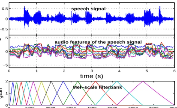
We exploit the non-linear resolution of the human auditory system across an audio spectrum using the Mel-scale filterbank analysis. We denote Fl as the group of the frequency bins
spanned by thel-th filter. The mono power spectrum is mapped into these filters to abtain the L-dimensional audio feature
aT(t) = [aT1(t), ..., aTL(t)]T for statistical training, where aTl(t) = log
X
f∈Fl
bl(f)|ST(f, t)|2, (7)
andbl(f)is the magnitude of the l-th filter whileST(f, t)is
the spectral component of the training audio. Figure 1 shows a typical speech signal and its audio features after the Mel-scale filterbank analysis. −0.5 0 0.5 time (s) speech signal 0 1 2 3 4 5 6 −5 0 5 time (s) magnitude
audio features of the speech signal
0 1000 2000 3000 4000 5000 6000 7000 8000 0 1 2 frequency (Hz) gain Mel−scale filterbank
Fig. 1. The speech signal and its audio features obtained by the filterbank analysis.
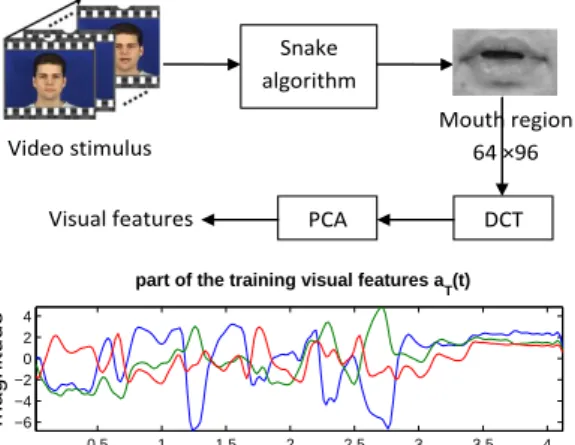
For the visual features, first we crop an area from the video to get the gross mouth region. We then use snakes [14] to detect the mouth contour. Snakes, also called active contour model, is an energy mimization process to delineate an object outline. Then we relocate the mouth centre and extract a64×
96 mouth region based on the contour. Then the fast block discrete cosine transform (DCT) is employed on the mouth region to compress the image. Finally principal component analysis (PCA) is applied to the DCT data to get the visual feature vector vT(t). In the experiment, we used 3 principal
components as visual features, which took up to 64.8% total variance. Figure 2 shows the detailed visual feature extraction process. Video stimulus Snake algorithm Mouth region 64 ×96 DCT PCA Visual features 0.5 1 1.5 2 2.5 3 3.5 4 −6 −4 −2 0 2 4 time (s) magnitude
part of the training visual features aT(t)
Fig. 2. The visual feature extraction process and part of the training visual featuresaT(t).
B. Feature Fusion
Using the audio feature vector aT(t) =
[aT1(t),· · · , aTL(t)]T obtained by theL Mel-scale filterbank
analysis, we synchronize and concatenate the visual feature vector with each element of the audio feature vector to form
L sets of audio-visual vector uTl(t) = [vT(t);aTl(t)]. The
objective of the training process is to obtain the parameter setλli={γli,µli,Σli} associated with eachuTl(t).
After independent GMM training,L×Iparameter sets{λli}
are estimated by the expectation maximization algorithm for each speaker.
IV. INDETERMINACIESCANCELLATIONALGORITHM
The indeterminacies cancellation algorithm is based on co-herence maximization. Suppose the separation succeeds with-out any permutation or scaling ambiguity, thenyk(n) =sk(n), yk(n) will have maximum coherence with its corresponding
video signalvk(t). Treating the frequency bin group f ∈ Fl
as a whole, we can maximize the following criterion in the frequency domain to address the indeterminacies:
[ ˆP(Fl),Dˆ(Fl)] = arg max P(Fl),D(Fl) X t K X k=1 logpAV(ukl(t)), (8)
where ukl(t) = [vk(t);akl(t)] is the audio-visual feature,
vk(t) is the visual feature associated with the k-th speaker
at time framet, andakl(t)is the audio feature extracted from
thek-th source estimate corresponding to thel-th filterbank. To estimate s1(n) from the observations, we can get the
separation vector p(Fl) and the scale parameter α(Fl) by
maximizing: [ˆp(Fl),αˆ(Fl)] = arg max p(Fl),α(Fl) X t logpAV(u1l(t)). (9)
A. Permutation Indeterminacy Cancellation
In equation (8), the direct summation of log-likelihood is very sensitive to outliers. It happens that one outlier may change the total summation greatly and result in a wrong decision. To deal with this problem, we propose a new sorting scheme. For convenience, we present an example of the 2×2 case:
1. Extract the visual features v1(t) and v2(t) from the video signal associated with the two speakers.
2. Extract the audio featuresa1(t)anda2(t)fromY1(f, t)
andY2(f, t)respectively.
3. Get the audio-visual data ukl(t) = [vk(t);akl(t)] and
uk†l(t) = [vk(t);ak†l(t)], (where k= 1,2, l = 1, ..., L, and †denotes the permutation version, 1† = 2,2† = 1).
4. Calculate the audio-visual probability pAV(ukl(t))and pAV(uk†l(t))based on the GMM model in equation (6) and the parameter set{λil}k associated with each speaker that has
been estimated in the training stage. 5. Define a criterion: J(l, t)def= 1, P klogpAV(ukl(t))> P klogpAV(uk†l(t)) 0, P klogpAV(ukl(t))<PklogpAV(uk†l(t)) . 6. IfPT
t=1J(l, t)> T /2, do nothing; otherwise, swap the
rows of W(f) (i.e.W(f)←−[0 1
1 0]W(f)), andY(f, t) for
f ∈ Fl.
In step 5, we have used a new criterion instead of the cumulative log-likelihood, to avoid the influence of outliers as in [11], which is equivalent to majority voting over time frames. For the sake of accuracy, we can iterate steps 2 to 6.
B. Scaling Indeterminacy Cancellation
Suppose we are now interested in addressing the scaling am-biguity of source estimate y1(n). IfY1‡(f, t) =α(Fl)Y1(f, t)
is the exact copy of the source speechS1(f, t)forf ∈ Fl
with-out any scaling amplification, i.e.,Y1‡(f, t) =S1(f, t),for f ∈
Fl, then this combines with equation (7) to give T X t=1 a‡l(t) = 2Tlog|α(Fl)|+ T X t=1 al(t). (10)
Therefore we can calculate Fl spanned by each filter:
α(Fl) = exp ( XT t=1 a‡l(t)− T X t=1 al(t) /(2T) ) . (11) PT
t=1al(t)is straightforward to calculate, and the priority is
on the estimation of PT
t=1a
‡
l(t)from the given visual vector
v(t). First we need to get the marginal probability density of the visual feature corresponding to each filterbankl:
pV(v(t)|l) = I
X
i=1
γliVN(v(t)|µliV,ΣliV), (12)
where γliV is the weighting parameter, µliV is the mean
a‡l(t)can be estimated as: a‡l(t) = I X i βli(t)µliA, (13)
whereµliA is the mean parameter of the audio feature al(t)
for thei-th kernel, and
βli(t) =
γlipV(v(t)|i)
P
jγljpV(v(t)|j) .
Then from equation (11) we can estimateα(Fl). In such a way,
we getLscale parameters, and each one affects the frequency bins spanned by one filter.
However, adjacentFloverlap with each other, and we
can-not define two scale parameters for an overlapped frequency bin. To solve this problem, we smooth between the L scale parameters with linear interpolation, as shown in Figure 3.
1 2 L 1 ( ) 2 ( ) ( L) ••• ••• ••• ••• Frequency (Hz) f
••• Smooth the L scale parameters {(l)} to get the final ( )f (the red curve)
Overlap
Fig. 3. Smooth betweenα(Fl)to obtainα(f).
V. EXPERIMENTALRESULTS
We tested the proposed algorithm on the XM2VTS [15] multi-modal database. The frontal face videos were captured at 25 fps and the speech signals were continuous sentences of words and digits recorded at 32 kHz. For each speaker, there are 24 recordings repeating 3 sentences. We trained the audio-visual coherence model of one target speaker with audio-audio-visual speech lasting for 41 seconds. The audio was downsampled to 16 kHz, and the 32 ms (512 samples) Hamming window with 12 ms overlap was used in the STFT. Audio features were extracted from 24 Mel-scaled filter banks. We chose the first 3 principal components from the video as the visual features, and they were upsampled to 50 Hz to be synchronized with the audio features.
To test the performance of the permutation cancellation algorithm, the speech signal from the target speaker and another interference speech signal randomly chosen from 96 audio signals by 4 other speakers were transformed into the time-frequency domain by the STFT. We swapped the spectral components of consecutive frequency bins of a filter. Then we calculated the accuracy rate of the permutation cancellation with different frame numbersT. In Figure 4, each
0 20 40 60 80 100 0.65 0.7 0.75 0.8 0.85 0.9 0.95 1
Time frame used T
permutation accuracy (%)
speaker1 speaker2 speaker3 speaker4
Fig. 4. The permutation accuracy with different time frames.
curve represents the comparison of the target speaker with an interference speaker. The result is an average of 24 mixtures. To test the scaling cancellation, we amplified the spectral components from the target speaker with different scaling parameters d(f) at different frequency bins. If the scaling problem was solved successfully, we should get α(f) that satisfiesα(f)·d(f) = 1. Figure 5 shows the real and estimated scaling factors α(f) with the algorithm described in section 3. The solid curve (estimatedα(f)·d(f)) in the lower part is close to 1, so we have mitigated the scaling problem greatly.
0 1 2 3 4 d(f) α(f) 0 1000 2000 3000 4000 5000 6000 7000 8000 0 1 2 3 4 freuqency (Hz) magnitude ideal d(f)*α(f) estimated d(f)*α(f)
Fig. 5. The scaling cancellation results.
We then tested the algorithm with convolutive mixtures synthesized on a computer. The filters {hpk} were generated
by the system utilizing the impulse response measurements of a conference room [16] with various positions of the microphones and the speakers. Two audio signals with each lasting 4 s were convolved with the filters to generate the mixtures.
We used the signal to interference ratio (SIR) at different signal to noise ratios (SNRs) as a criterion to evaluate the performance of our bimodal BSS algorithm. Based on the
extraction ofs1(n)from the observations, we have SIR= 10 log P nk PP p=1w1p(n)∗hp1(n)∗s1(n)k P nkˆs1(n)−P P p=1w1p(n)∗hp1(n)∗s1(n)k . (14) The degradation of convolutive BSS performance is maily caused by the permutation problem. From the upper half of ta-ble I, we found that after applying the permuation cancellation algorithm with the sorting scheme in section IV-A, SIRs of the source signal were improved greatly in a wide range of noise levels, with the highest point at about 20dB. In this table, the input SNR is the ratio between the audio signals and gaussian noise, i.e. energy(s1+s2)/energy(noise), and the input SIR
is the ratio between a target signal and the interference, i.e. energy(s1)/energy(s2+noise). The output SIR was caculated
by equation (14). In the lower half of table I, after permuation indeterminacy cancellation, the scaling ambiguity cancellation algorithm was applied to the realigned spectral components, which improved the performance in high noise environment.
TABLE I
OUTPUTSIR (dB)COMPARISON.
10 15 20 25 30 -1.42 -0.91 -0.74 -0.68 -0.66 before sorting 4.02 6.40 8.81 13.41 13.24 after sorting 5.29 9.28 12.97 14.66 14.8 4 6 8 10 12 -3.13 -2.38 -1.82 -1.42 -1.15 before scaling 0.66 2.07 3.83 5.29 6.77 after scaling 2.07 3.71 4.55 5.82 6.80 Input SIR Output SIR
Evaluation of Permutation Indeterminacy Cancellation Input SNR
Input SIR Output SIR
Evaluation of Scaling Indeterminacy Cancellation Input SNR
VI. CONCLUSION
We have presented a new audio-visual convolutive BSS system. In this system, we have combined the audio features with visual features to form an audio-visual feature space. A new sorting scheme exploiting the audio-visual coherence to solve the permutation indeterminacy problem has also been presented. We also provided a new method to estimate the power spectrum to mitigate the scaling ambiguity. Our algorithm has been tested on the XM2VTS database and has shown good performance.
ACKNOWLEDGMENT
This work was supported by the Engineering and Phys-ical Sciences Research Council (EPSRC) (Grant number EP/H012842/1) and the MOD University Defence Research Centre on Signal Processing (UDRC).
REFERENCES
[1] Schwartz, J.L., Berthommier, F. and Savariaux, C., “Seeing to Hear Better: Evidence For Early Audio-visual Interactions in Speech Iden-tification.”,Cognition, vol. 93, pp. B69–78, Sep. 2004.
[2] Jutten, C., Herault, J.: “Blind Separation of Sources, Part I: An Adaptive Algorithm Based on Neuromimetic Architecture.”Signal Process.vol. 24, no. 1, pp. 1–10, 1991.
[3] Cardoso, J.F., Souloumiac, A.: “Blind Beamforming for Non-Gaussian Signals.”IEEE Proc.-F,vol. 140, no. 6, pp. 362–370, 1993.
[4] Comon, P., “Independent Component Analysis, a New Concept?”,Signal Process., vol. 36, pp. 287–314, 1994.
[5] Anem¨uller, J., Kollmeier, B.: “Amplitude Modulation Decorrelation for Convolutive Blind Source Separation.” In:Proc. ICA, pp. 215–220, 2000. [6] Ikram, M.Z., Morgan, D.R.: “A Beamforming Approach to Permutation Alignment for Multichannel Frequency-Domain Blind Speech Separa-tion.” InProc. IEEE ICASSP, pp. 881–884, 2002.
[7] Sawada, H., Mukai, R., Araki, S., and Makino, S., “A Robust and Precise Method for Solving the Permutation Problem of Frequency-Domain Blind Source Separation”,IEEE Trans. Speech Audio Process., vol. 12, pp. 530–538, 2004.
[8] Thomas, J., Deville, Y., Hosseini, S.: “Time-Domain Fast Fixed-Point Algorithms for Convolutive ICA.”IEEE Signal Process. Lett., vol. 13, no. 4, pp. 228–231, 2006.
[9] Wang, W., Cosker, D., Hicks, Y., Sanei, S. and Chambers, J., “Video Assisted Speech Source Separation”, inProc. IEEE ICASSP, pp. 425– 428, 2005.
[10] Rivet, B., Girin, L. and Jutten, C., “Mixing Audiovisual Speech Process-ing and Blind Source Separation for the Extraction of Speech Signals from Convolutive Mixtures”,IEEE Trans. Audio Speech Lang. Process., vol. 15, pp. 96–108, 2007.
[11] Liu, Q., Wang, W. and Jackson, P., “Use of Bimodal Coherence to Resolve Spectral Indeterminacy in Convolutive BSS”, inProc. LVA/ICA
2010.
[12] Liu, Q., Wang, W. and Jackson, P., “Bimodal Coherence based Scale Ambiguity Cancellation for Target Speech Extraction and Enhance-ment”, inProc. Interspeech2010.
[13] Casanovas, A.L., Monaci, Gianluca., Vandergheynst, P. and Gribonval, R., “Blind Audiovisual Source Separation Using Overcomplete Dictio-naries”, inProc. IEEE ICASSP, 2008.
[14] Kass, M., Witkin, A. and Terzopoulos, D., “Snakes: Active Contour Models”,International Journal of Computer Vision, pp. 321–331, 1988. [15] Messer, K., Matas, J., Kittler, J., Luettin, J., Maitre, G.: XM2VTSDB: The Extended M2VTS Database. In: AVBPA, 1999. [Online] Available: http://www.ee.surrey.ac.uk/CVSSP/xm2vtsdb/
[16] Westner, A.: Room Impulse Responses, 1998. [Online] Available: http: //alumni.media.mit.edu/∼westner/papers/ica99/node2.html