RESEARCH ARTICLE
Randomized SMILES strings improve
the quality of molecular generative models
Josep Arús‑Pous
1,3*, Simon Viet Johansson
1, Oleksii Prykhodko
1, Esben Jannik Bjerrum
1, Christian Tyrchan
2,
Jean‑Louis Reymond
3, Hongming Chen
1and Ola Engkvist
1Abstract
Recurrent Neural Networks (RNNs) trained with a set of molecules represented as unique (canonical) SMILES strings, have shown the capacity to create large chemical spaces of valid and meaningful structures. Herein we perform an extensive benchmark on models trained with subsets of GDB‑13 of different sizes (1 million, 10,000 and 1000), with different SMILES variants (canonical, randomized and DeepSMILES), with two different recurrent cell types (LSTM and GRU) and with different hyperparameter combinations. To guide the benchmarks new metrics were developed that define how well a model has generalized the training set. The generated chemical space is evaluated with respect to its uniformity, closedness and completeness. Results show that models that use LSTM cells trained with 1 million randomized SMILES, a non‑unique molecular string representation, are able to generalize to larger chemical spaces than the other approaches and they represent more accurately the target chemical space. Specifically, a model was trained with randomized SMILES that was able to generate almost all molecules from GDB‑13 with a quasi‑uniform probability. Models trained with smaller samples show an even bigger improvement when trained with randomized SMILES models. Additionally, models were trained on molecules obtained from ChEMBL and illustrate again that train‑ ing with randomized SMILES lead to models having a better representation of the drug‑like chemical space. Namely, the model trained with randomized SMILES was able to generate at least double the amount of unique molecules with the same distribution of properties comparing to one trained with canonical SMILES.
Keywords: Deep learning, Generative models, SMILES, Randomized SMILES, Recurrent Neural Networks, Chemical databases
© The Author(s) 2019. This article is distributed under the terms of the Creative Commons Attribution 4.0 International License (http://creat iveco mmons .org/licen ses/by/4.0/), which permits unrestricted use, distribution, and reproduction in any medium, provided you give appropriate credit to the original author(s) and the source, provide a link to the Creative Commons license, and indicate if changes were made. The Creative Commons Public Domain Dedication waiver (http://creativecommons.org/ publicdomain/zero/1.0/) applies to the data made available in this article, unless otherwise stated.
Introduction
Exploring the unknown chemical space in a meaning-ful way has always been one of the major objectives in drug discovery. Given the fact that the drug-like chemi-cal space is enormous (the lower estimation is 1023 mol-ecules) [1], it cannot be easily searched. One of the most interesting attempts to understand the chemical space is the GDB project [2], which encompasses a set of data-bases that combinatorially enumerate large parts of the small molecule fragment-like chemical space. Currently there are databases that enumerate most fragment-like molecules with up to 13 (975 million molecules) [3] and
17 (166 billion molecules) [4] heavy atoms. Another approach, GDB4c [5], enumerates ring systems up to four rings both in 2D (circa one million ring systems) and 3D (more than 6 million structures). Although managing billion-sized databases is computationally challenging, the enumerative approach has proven useful to study the entire small drug-like molecular chemical space in an unbiased way [6].
In the last 2 years molecular deep generative models have emerged as a powerful method to generate chemi-cal space [7] and obtain optimized compounds [8]. Given a training set with molecules (generally a database such as ChEMBL [9]), these models learn how to create mol-ecules that are similar but not the same as those in the training set, thus spanning a bigger chemical space than that of the training data. Either after or during training, the probability of generating molecules with specific
Open Access
*Correspondence: [email protected]
1 Hit Discovery, Discovery Sciences, R&D, AstraZeneca Gothenburg,
Mölndal, Sweden
Full list of author information is available at the end of the article
source:
https://doi.org/10.7892/boris.138507
properties can be altered with techniques such as rein-forcement [8] or transfer learning [7, 10]. Multiple archi-tectures have been reported in literature: the first one is Recurrent Neural Networks (RNNs) [7], but also others such as Variational AutoEncoders (VAEs) [11], Genera-tive Adversarial Networks (GANs) [12, 13], etc. [14]. Due to its simplicity, in most published research the format representing molecules is the canonical SMILES nota-tion [15], a string representanota-tion unique to each mole-cule. Nevertheless, models that use the molecular graph directly are starting to gain interest [16, 17].
Notwithstanding the popularity of RNNs, the idi-osyncrasies of the canonical SMILES syntax can lead to training biased models [18]. Specifically, models trained with a set of one million molecules from GDB-13 have a higher probability of generating molecules with fewer rings. Additionally, the canonical SMILES representation can generate substantially different strings for molecules that are very similar, thus making some of them more dif-ficult to sample. To prove this, these models were sam-pled with replacement 2 billion times and at most only 68% of GDB-13 could be obtained from a theoretical maximum of 87%. This maximum would be from sam-pling with replacement the same number of times from a theoretical ideal model that has a uniform probability of obtaining each molecule from GDB-13, thus obtaining the least possible biased output domain.
We performed an extensive benchmark of RNN mod-els trained with SMILES obtained from GDB-13 whilst exploring an array of architectural changes. First and foremost, models were trained with three different variants of the SMILES notation. One of them is the commonly used canonical SMILES, another one are ran-domized SMILES (also known as enumerated SMILES), which have been used as a data amplification technique
and are shown to generate more diversity in some model architectures [19–21]. The third one is DeepSMILES [22], a recently published modification of the canoni-cal SMILES syntax. Secondly, models were trained with decreasing training set sizes (1,000,000, 10,000 and 1000 molecules) to explore the data amplification capa-bilities of randomizes SMILES. Thirdly, the two most used recurrent cell architectures were compared: long short-term memory (LSTM) [23] and Gated Recurrent Unit (GRU) [24]. GRU cells are widely used as a drop-in replacement of LSTM cells with an noticeable speed improvement, but it has been shown that in some tasks they perform worse [25]. Fourthly, regularization tech-niques such as dropout [26] in conjunction with different batch sizes were also tested and their impact on the gen-erated chemical space assessed. All of the benchmarks were supported by a set of metrics that evaluate the uni-formity, completeness and closedness of the generated chemical space. With this approach, the generated chem-ical space is treated as a generalization of the training set to the entire GDB-13 and the chemical space exploration capability of the models can be assessed. Finally, to dem-onstrate how the same methodology can be used to train models that generate real-world drug-like compounds, models were trained with a subset of the ChEMBL [9] database.
Methods
Randomized SMILES strings
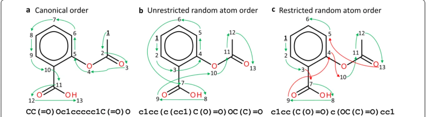
To obtain canonical SMILES the atoms in a given mol-ecule have to be uniquely and consistently numbered. In the case of RDKit this is done by using a modified ver-sion of the Morgan algorithm [27, 28]. The SMILES generation algorithm is then able to traverse the molec-ular graph always in the same way (Fig. 1a). Some atom
CC(=O)Oc1ccccc1C(=O)O c1cc(c(cc1)C(O)=O)OC(C)=O c1cc(C(O)=O)c(OC(C)=O)cc1 1 2 3 4 5 6 7 8 9 10 11 12 13 12 11 13 10 4 5 6 1 2 3 7 9 8 12 11 13 10 4 5 6 1 2 3 7 9 8
Canonical order Unrestricted random atom order Restricted random atom order
a b c
Fig. 1 Traversal of the molecular graph of Aspirin using three methods: a the canonical ordering of the molecule; b atom order randomization without RDKit restrictions; c Atom order randomization with RDKit restrictions of the same atom ordering as b. Atom ordering is specified with a number ranking from 1 to 13 for each atom and the arrows show the molecular graph traversal process. Notice that the atom ordering is altered in c, prioritizing the sidechains (red arrows) when traversing a ring and preventing SMILES substrings like c1cc(c(cc1))
orderings can lead to overly complicated SMILES strings and that is why RDKit has some built-in fixes that alter atom order on-the-fly. They prevent strange combina-tions, such as prioritizing traversing sidechains before the ring atoms, and are by default active.
One easy way of obtaining randomized SMILES is by randomizing atom ordering. This does not alter how the algorithm traverses the graph (i.e., depth-first in the case of RDKit), but changes the starting point and in what order the branching paths are selected. With this approach, theoretically, at most n! different SMILES
can be generated on a molecule with n heavy atoms, yet the resulting number of different combinations ends up being much lower. The two different variants of ran-domized SMILES used here (Fig. 1b, c) only change on the application of the RDKit fixes. This makes the unre-stricted version a superset of the reunre-stricted one, which includes the SMILES that are disallowed in the regular restricted version.
RNNs trained with SMILES Pre‑processing SMILES strings
SMILES strings of all variants need to be tokenized to be understood by the model. Tokenization was performed on a character basis with the exception of some specific cases. The first are the “Cl” and “Br” atoms, which are two-character tokens. Second are atoms with explicit hydrogens or charge, which are between brackets (e.g., “[nH]” or “[O-]”). Third, ring tokens can be higher than 9 in which case the SMILES syntax represents the num-ber prepended with the “%” character (e.g., “%10”). These rules apply to all SMILES variants used in this research. Lastly, the begin token “^” was prepended and the end token “$” appended to all SMILES strings. The tokeniza-tion process was performed independently for each data-base and yielded vocabulary sizes of 26 in GDB-13 and 31 in ChEMBL. When training the DeepSMILES models, the official implementation [22] was used to convert the SMILES.
Architecture
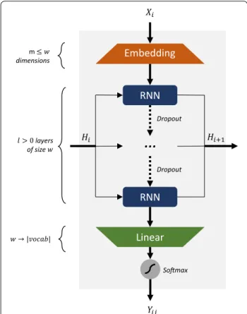
The model architecture used is similar to the one used in [7, 8, 18] and is illustrated in Fig. 2. The training set sequences are pre-processed, and for each training epoch the entire training set is shuffled and subdivided in b batches. The encoded SMILES strings of each batch are fed token by token to an embedding layer of m
dimen-sions, followed by l layers of LSTM [23] /GRU [24] cell
size w . To prevent squeezing the encoded input, the embedding dimensions should be m≤w . Between the inner RNN layers there can be dropout layers [26] with a probability d . The output from the cells is squeezed to the vocabulary size v by a linear transformation layer and
a softmax is performed to obtain the probabilities of sam-pling each token in the next position. This is repeated for each token in the entire sequence.
Training a model
Following [18], all models have two sets: a training and a validation set. The validation set holds molecules that are in the target chemical space but are not used for training the model. Depending on the training set different splits can be made. In Table 1 is shown the size of the training and validation sets for each of the benchmarks (see Additional file 1: Methods S1 for more information on how the databases were filtered). In the case of models trained with randomized SMILES, a new sample of randomized SMILES of the same molecules are used for the training and validation set for each epoch. These training set files are created beforehand and the model uses a different file for each epoch. For example, a model trained with one million molecules
RNN RNN Linear Embedding Dropout Dropout Somax
…
> 0 layers of size m dimensions | |Fig. 2 Architecture of the RNN model used in this study. For every step i , input one‑hot encoded token Xi goes through an embedding
layer of size m≤w , followed by l>0 GRU/LSTM layers of size w with dropout in‑between and then a linear layer that has dimensionality w
and the size of the vocabulary. Lastly a softmax is used to obtain the token probability distribution Yij . Hi symbolizes the input hidden state matrix at step i
for 300 epochs will have approximately 300 million dif-ferent randomized SMILES, although the number is generally lower because some SMILES are more com-monly sampled than others.
During each epoch the training set is shuffled and minibatches of size b are created. These batches are in the form of a matrix with a row for each encoded SMILES string and appended with end tokens as pad-ding. The “teacher’s forcing” approach is used in train-ing, which means that the correct token is always input in the next step, regardless of the prediction from the model [29]. The loss function to minimize by the model is the average negative log-likelihood (NLL) of the entire batch of tokenized SMILES strings. Given Xi and xi as the sampled and expected token at previous step i≥0 respectively and the current time step T ≥0 , the partial NLL of a SMILES string is computed as:
To prevent instability during training, the computed gradients are updated so that the norm is 1.0 . When performing a forward-pass on a batch, the model does not apply any mask to already finished sequences. This makes the model run slightly faster because no masks are computed and, as the padding token is the end of sequence, it does not affect the quality of the train-ing process. All weight matrices are initialized from a uniform random distribution U
−√1/w,√1/w . The learning decay strategy is based on a custom metric calculated at each epoch (UC-JSD) and is discussed in section “Adaptive learning rate decay strategy” of the Additional file 1: Methods S2.
Benchmark
The models were optimized over the hyperparam-eter combinations shown in Table 2. The two models with bigger training set sizes were optimized for fewer
J(T)=NLL(T)= −lnP(X0=xo) − T t=1 lnP(Xt=xt|Xt−1=xt−1. . .X1=x1)
parameters, as training times were much longer. On the other hand, the two smaller models allowed for more optimizations, as each epoch took few seconds to calcu-late. After the first benchmark, GRU cells were dropped because of their consistently lower performance.
After each hyperparameter optimization, the best epoch was chosen as follows. A smoothing window func-tion size 4 was applied to the UC-JSD calculated on each epoch, selecting the epoch with the lowest UC-JSD (see next section) as the best one.
UC‑JSD—a metric for generative models
The metric used for the benchmark is derived from pre-vious research [18]. There, it was hypothesized that the best models are those in which the validation, train-ing and sampled set NLL distributions are uniform and equivalent. The Jensen–Shannon Divergence (JSD) meas-ures the divergence between a set of probability distribu-tions [30] and is calculated as:
where H(d) is the Shannon entropy of a given probabil-ity distribution and ∀d∈D;0< αd <1 and
αd =1 are weights. The JSD→0 when ∀di∈D;di=dj;i�=j , which does not explicitly consider uniformity (i.e., the distributions can be non-uniform but equal).
To solve this issue the Uniformity–Completeness JSD (UC-JSD) was designed. Instead of binning the raw distribution NLLs, each of the NLLs is used as it is. Given the three NLL vectors for the sampled, training and validation sets of the same size NLLS=NLLvalidation,NLLtraining,NLLsampled
and αi=1/3 , the values in each vector are divided by the
total sum, giving a probability distribution with as many val-ues as items in the vector. Then (Eq. 1 is used to calculate the JSD between the three distributions. Notice that, since the model is sampled randomly, the UCJSD→0 either in the highly unlikely case that all the samples have molecules with (1) JSD=H d∈D αi·di − d∈D αiH(di) Table 1 Training and validation set sizes for the different
benchmarks
Notice that depending on the expected size of the target chemical space and the total amount of molecules, different ratios have been used
Model Training set size Validation set size
GDB‑13 1M 1,000,000 10,000
GDB‑13 10K 10,000 1000
GDB‑13 1K 1000 1000
ChEMBL 1,483,943 78,102
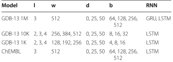
Table 2 Hyperparameter combinations used in the grid search
Number of layers (l), dimensions of the RNN layers (w), dropout rate % (d), batch size (b), RNN cell type (RNN)
Model l w d b RNN GDB‑13 1M 3 512 0, 25, 50 64, 128, 256, 512 GRU, LSTM GDB‑13 10K 2, 3, 4 256, 384, 512 0, 25, 50 8, 16, 32 LSTM GDB‑13 1K 2, 3, 4 128, 192, 256 0, 25, 50 4, 8, 16 LSTM ChEMBL 3 512 0, 25, 50 64, 128, 256, 512 LSTM
the same NLL or all three distributions are uniform, and the model is complete.
Sampling the best epoch of a model
The main objective of sampling a model is to assess the properties of the output domain. Namely, in the case of GDB-13, the uniformity (equal probability of sampling), completeness (sampling all molecules from GDB-13) and closedness (only molecules from GDB-13 are sampled) are to be assessed. To ease the evaluation of the models, three ratios representing the three properties were defined.
Given a sample with replacement size k , the valid (SMILES parsed correctly with repeats), in (SMILES with
repeats in GDB-13), unique (sampled unique canoni-cal SMILES in GDB-13) subsets are obtained. Both ratiovalid = |validk | and ratioin= |in|k are relative to the entire sample but ratiounique= ||GDBunique13|| is relative to ϕ(k) , which represents the expected ratio of different molecules obtainable when a sample size k with replacement is per-formed on a model that generates uniformly all mole-cules from and only from GDB-13 (ideal model) [18] (i.e., ϕ2·109
=0.8712 ). This allows to define the ratios as:
Also, the UCC=completeness·uniformity·closedness was also defined as a unified score that heavily penalizes
completeness= ratiounique ϕ(k)
uniformity= ratiounique
ϕ(|in|)
closedness=ratioin
models that have low scores. See the Additional file 1: Methods S2–4 for further details on how the benchmark was performed.
Technical notes
All the software was coded in Python 3.6.8. The models were coded using the PyTorch 1.0.1 library [31]. Unless specified, the chemistry library used throughout is RDKit 2019_03_01 [32] and for all the big data processing Spark 2.4.3 [33] was used. All plots were made with matplot-lib 3.0.3 [34] and seaborn 0.9.0 [35]. The GPU hardware used to train and sample the models were Nvidia Tesla V100 (Volta) 16 GB VRAM cards using CUDA 9.1 on stable driver 390.30. The MOSES and FCD benchmarks were calculated using the code provided in (https ://githu b.com/molec ulars ets/moses ).
Results
Optimizing generative models with 1 million SMILES from GDB‑13
Canonical vs. randomized SMILES
Hyperparameter optimizations of the three main SMILES variants (canonical, randomized restricted and rand-omized unrestricted) were performed on models trained with 1 million molecules randomly sampled from GDB-13 (Table 2). A k=2·109 SMILES sample was per-formed on the best epoch for each of the models trained in the benchmark (see Additional file 1: Methods S1). Results show (Table 3, Additional file 2: Figure S4 for the best hyperparameter combinations for each SMILES type and Additional file 3: Table S1 for all results) that the ran-domized variants greatly outperform canonical SMILES. The best canonical SMILES model was only able to
Table 3 Best models trained on subsets of GDB-13 after the hyperparameter optimization
See “Methods” section for a description of the ratios Best result for each training set size are indicated in italics
Set Benchmark training set size, SMILES SMILES variant, including randomized variants with and without data augmentation (DA), Time training time up in hh:mm, % GDB-13 Percent of unique molecules from GDB‑13 generated in a 2 billion sample with replacement, Valid valid SMILES, Unif uniformity ratio, Comp completeness ratio, Closed closedness ratio, UCC UCC ratio
Set SMILES Time % GDB‑13 Valid Unif Comp Closed UCC
1M Canonical 4:08 72.8 0.994 0.879 0.836 0.861 0.633 Rand. unr. 31:47 80.9 0.995 0.970 0.929 0.876 0.790 Rand. unr. no DA 1:37 77.0 0.987 0.957 0.795 0.883 0.672 Rand. rest. 7:19 83.0 0.999 0.977 0.953 0.925 0.860 Rand. rest. no DA 1:21 78.2 0.992 0.957 0.829 0.898 0.712 DS branch 1:33 72.1 0.987 0.881 0.828 0.834 0.608 DS rings 1:11 68.6 0.979 0.852 0.788 0.798 0.535 DS both 1:05 68.4 0.979 0.851 0.785 0.796 0.532 10K Canonical 0:04 38.8 0.905 0.666 0.445 0.426 0.126 Rand. rest. 0:36 62.3 0.974 0.882 0.715 0.598 0.377 1K Canonical 0:01 14.5 0.504 0.611 0.167 0.133 0.014 Rand. rest. 0:04 34.1 0.812 0.790 0.392 0.276 0.085
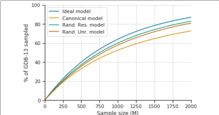
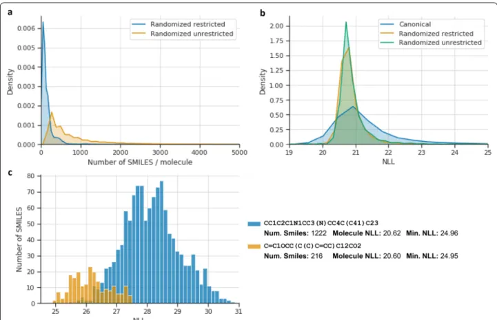
enumerate 72.8% of GDB-13 compared to the 83.0% of the restricted randomized SMILES (Fig. 3). All three metrics, uniformity, completeness and closedness are much higher and show that the restricted randomized models are theoretically able to generate most of GDB-13 with uniform probability. This can be further seen in Fig. 4b, where the NLL distribution of a sample of mole-cules from the GDB-13 randomized SMILES models is centered at NLLGDB13= −ln 1 |GDB13| =20.6 and is much narrower than that of the canonical variant model.
Comparing the two variants of randomized SMILES, models trained with both variants have a similarly uni-form output domain (Fig. 4b), but models trained with restricted randomized variant have a more complete and more closed domain than those trained with the unrestricted variant. The output domain of the ideal randomized SMILES models would comprise all pos-sible SMILES strings of any given variant pospos-sible to be generated from all molecules in GDB-13. This con-trasts with the canonical model, in which the output domain is one SMILES per molecule. Each molecule has a different number of SMILES strings, depending on its topology, although only a few (generally highly cyclic or branched molecules) have numbers above 1000 (Fig. 4a). Knowing that the training objective is to obtain a uniform posterior distribution, it would be expected that molecules with more randomized
SMILES should have a higher probability of being sam-pled than those that have fewer. However, this is never the case as models trained with randomized SMILES have a much more uniform posterior probability dis-tribution than those trained with canonical SMILES (Fig. 4b). The model naturally learns to prioritize some SMILES in molecules with a large number of possi-ble SMILES, and to have a more uniform distribution among all possible SMILES on molecules that have less. This can be seen in Fig. 4c, where two molecules have the same NLL, but one (blue) has six times the number of possible SMILES than the other (orange).
Models trained with randomized SMILES without data augmentation (the same SMILES strings each epoch) were also benchmarked. Results show (Table 3, Addi-tional file 2: Figure S4 for the best hyperparameter com-binations for each SMILES type and Additional file 3: Table S1 for all results) that they perform better than the models trained with canonical SMILES but worse than those with data augmentation. This indicates that not using the canonical representation constraint makes bet-ter models, but also that data augmentation has a positive impact on the training process.
DeepSMILES is a SMILES syntax variant that alters the syntax and changes how rings and branching are repre-sented [22]. Three different forms of DeepSMILES were explored: one with the new ring syntax, another with the
Fig. 3 Plot illustrating the percent of GDB‑13 sampled alongside the sample size of the ideal model (blue) and the best of the canonical (yellow), randomized restricted (green) and randomized unrestricted (orange) models. Notice that the ideal model is always an upper bound and eventually ( n∼21B ) would sample the entire GDB‑13. The trained models would reach the same point much later
new branching syntax and a last one with both changes. Results show (Table 3, Additional file 3: Table S1 com-plete) that the performance is consistently lower than using normal canonical SMILES. The validity is generally 1–3% lower than in canonical SMILES, possibly indicat-ing that the model has difficulties in learnindicat-ing the basics of the syntax.
The hyperparameter optimization also gives some hints on how dropout, batch size and cell type affect the training process, although it varies for each SMILES variant. Plots for each hyperparameter compared to the four ratios and the training time were drawn (Addi-tional file 2: Figure S1) and show that adding drop-out only makes canonical SMILES models better. The model improves its completeness, but at the expense of closedness, meaning that it generates more molecules from GDB-13 at the expense of making more mistakes. On the other hand, larger batch sizes have generally a positive impact in models of all SMILES variants and
at the same time make training processes much faster. But the most interesting result is that the best models for all SMILES variants use LSTM cells. Moreover, even though the training time per epoch of the GRU cells is lower, LSTM models are able to converge in fewer epochs.
Similarity maps for the randomized SMILES were also plotted (Additional file 2: Figure S2) and confirm that models trained with randomized SMILES are able to generate mostly all molecules from GDB-13 with uni-form probability. Only molecules on the left tip of the half-moon (highly cyclic) are slightly more difficult to generate, but this is because they have extremely compli-cated SMILES with uncommon tokens and ring closures. Additionally, maps colored by the number of SMILES per molecule were created and show that most of the molecules that have more randomized SMILES are the same as those that are difficult to sample in the canonical models.
Fig. 4 Histograms of different statistics from the randomized SMILES models. a Kernel Density Estimates (KDEs) of the number of randomized SMILES per molecule from a sample of 1 million molecules from GDB‑13. The plot has the x axis cut at 5000, but the unrestricted randomized variant plot has outliers until 15,000. b KDEs of the molecule negative log‑likelihood (NLL) for each molecule (summing the probabilities for each randomized SMILES) for the same sample of 1 million molecules from GDB‑13. The plot is also cropped between range (19, 25) . c Histograms between the NLL of all the restricted randomized SMILES of two molecules from GDB‑13
UC‑JSD can be used to predict the best models
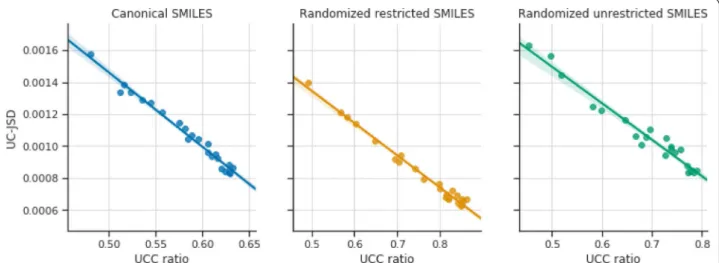
The previous benchmark employed an adaptive learning rate strategy (see Additional file 1: Methods S2) that uses the UC-JSD metric to evaluate the quality of the models and trigger a learning rate change. Moreover, the same metric was used to select the best epochs to perform a sample for each model. Plotting the UC-JSD against UCC shows a strong correlation in all three SMILES variants (Fig. 5). It is important to notice that the UC-JSD values should not be compared between models, as the out-put domain is different. This result shows that it is not necessary anymore to sample all models, but only the one that has the best UC-JSD. That is why for all future benchmarks only the model with the lowest UC-JSD is sampled. Moreover, the GRU cells have not shown any improvement whatsoever compared to the LSTM cells (Additional file 2: Figure S1) and the unrestricted randomized SMILES variant performs worse than the restricted variant. Henceforth, only the restricted variant of randomized SMILES and LSTM cells will be used for the next benchmarks.
Training generative models with smaller training sets To further show the data augmentation capabilities of randomized SMILES, two models were trained with 1000 and 10,000 molecules respectively, randomly obtained from GDB-13. Hyperparameter optimization was modi-fied to accommodate smaller training sets and, as mod-els were faster to train, different network topologies were tested (Table 2). When the training sets are so small, models are often unable to learn the syntax properly and thus generate more invalid structures. The model using 1000 molecules was the most affected by this problem,
with some models not even reaching 50% validity. This impacts the accuracy of the UC-JSD, because all mol-ecules tend to have a sampling probability p→0 . This makes the UC-JSD have low values because all molecules have very similar probability. For this reason, only models that had more than 50% valid SMILES were considered.
Results show (Table 3, Additional file 3: Table S1 com-plete) that models trained with randomized SMILES have better performance than those trained with canoni-cal SMILES. In the models trained with 1000 molecules, those with canonical SMILES are at most able to gener-ate up to 70% valid SMILES, although the best model was only able to generate 50% valid SMILES. Moreover, the completeness ratio of the best model is only 0.1325, meaning that most of the SMILES generated are not part of GDB-13: they correspond to molecules containing fea-tures excluded from GDB-13 (e.g. strained rings, unstable functional groups, wrong tautomer). Alternatively, the models trained with randomized SMILES show a much better behavior. Most models learn how to generate SMILES strings correctly (validity over 80%), complete-ness is much higher (0.2757) and their posterior distri-bution is more uniform. This is further illustrated with the fact that randomized SMILES models generate up to 34.11% of unique GDB-13 molecules and canonical mod-els only 14.54%.
Models trained with a bigger sample of 10,000 mol-ecules show similar trends but have much better perfor-mance in both cases. In this case, a model trained with randomized SMILES is able to uniquely generate 62.29% of GDB-13 while only training with less than 0.001% of the database, whereas a canonical SMILES model is only able to generate 38.77%. Closedness is much better in
Fig. 5 Linear regression plots between the UC‑JSD and the UCC ratio. a Canonical SMILES R2=0.931 . b Restricted randomized SMILES R2=0.856 . c Unrestricted randomized SMILES R2=0.885
both models: canonical SMILES models have at most 0.4262, whereas randomized SMILES models up to 0.5978. Lastly, a large number of SMILES generated are not included in GDB-13, meaning that the model, even though generating valid molecules, does not fully learn the specific idiosyncrasies of GDB-13 molecules and gen-erates valid molecules that break some condition. Improving the existing ChEMBL priors with randomized SMILES
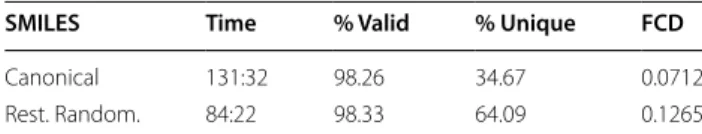
The same benchmark study was also performed on mod-els with a drug-like training set from ChEMBL (see Addi-tional file 1: Methods S1 for more information on how the training set was obtained). A different and reduced set of hyperparameter values were used due to long train-ing times (Table 2). The best models for both the canoni-cal and restricted randomized SMILES benchmarks were obtained using the same procedure as before and a 2 billion sample was performed. Results show (Table 4, extended results Additional file 3: Table S2) that the out-put domain of the canonical model is much smaller than that of the randomized SMILES model. Specifically, the randomized SMILES model can generate at least twice the number of different molecules than the canonical.
Nevertheless, the Fréchet ChemNet Distance (FCD) [36] between the validation set and a sampled set of 75,000 SMILES is lower on the canonical SMILES model. This could mean that the molecules generated by the canoni-cal model have more similar properties than ChEMBL molecules, but it could also mean that the canonical model overfits and generates molecules that are similar to the training set given that the validation set and the training set are biased the same way (i.e., they are both obtained from a biased sample of the entire drug-like chemical space).
To prove that the molecules sampled from the ran-domized SMILES model are at least as diverse as those in the canonical, several physicochemical properties and metrics (as used in the MOSES benchmark [37]), such as molecular weight, logP, Synthetic Accessibility Score (SA) [38], Quantitative Estimate of Drug-likeness Score (QED) [39], Natural-Product likeness score (NP) [40] and Internal Diversity (cross-molecule Tanimoto similarity on ECFP4) were calculated for a sample of the training, validation, randomized SMILES model and canonical SMILES model (Additional file 2: Figure S3). All of the plots are nearly identical, showing that there is no clear difference between molecules in any of the four sets. Additionally, molecule NLL plots for the same four sam-ples were calculated for both models (Fig. 6) and show that the canonical model greatly overfits the training and validation sets compared to the randomized SMILES model, which has mostly the same distribution for both sets. When comparing the two samples, the canonical model has much lower probabilities of generating most of the molecules generated by the randomized SMILES model, but not the opposite. The randomized SMILES model is able to generate the canonical SMILES model
Table 4 Best models from the ChEMBL benchmark
for both SMILES variants
SMILES SMILES variant, Time time used to train the model hhh:mm, % Valid Percent of valid molecules, % Unique Percent of unique molecules in a 2 billion SMILES sample, Fréchet ChemNet Distance (FCD) between the validation and a sample of 75,000 molecules (FCD)
SMILES Time % Valid % Unique FCD
Canonical 131:32 98.26 34.67 0.0712
Rest. Random. 84:22 98.33 64.09 0.1265
Fig. 6 Kernel Density Estimates (KDEs) of the Molecule negative log‑likelihoods (NLLs) of the ChEMBL models for the canonical SMILES variant (left) and the randomized SMILES variant (right). Each line symbolizes a different subset of 50,000 molecules from: Training set (green), validation set (orange), randomized SMILES model (blue) and canonical SMILES model (yellow). Notice that the Molecule NLLs for the randomized SMILES model (right) are obtained from the sum of all the probabilities of the randomized SMILES for each of the 50,000 molecules (adding up to 320 million randomized SMILES), whereas those from the canonical model are the canonical SMILES of the 50,000 molecules
molecules with higher likelihood than average, implying that the output domain of the canonical SMILES model is a subset of the randomized SMILES model output domain.
Discussion
Why are randomized SMILES better?
A SMILES molecular generative model learns by finding patterns in the SMILES strings from the training set with the goal of generalizing a model that is able to obtain all the SMILES in the training set with the highest possible probability. The procedure is exactly the same with any SMILES variant, the only thing that changes is the string representation of each molecule and, in the case of rand-omized SMILES, the number of different representations each molecule has. When the canonical representation is used, the model learns to generate one linear representa-tion of each molecule obtained through a canonicaliza-tion algorithm. This means that the model must learn not only to generate valid SMILES strings, but also to gener-ate those in the canonical form. As shown in “Methods” section (Fig. 1), the canonicalization algorithm in RDKit does not only traverse the molecule using a fixed order-ing, but also adds some restrictions on how to traverse rings. Moreover, models tend to see the same patterns repeatedly, leading to premature overfitting (Fig. 6). Alternatively, randomized SMILES models do not have the canonical form limitation and can learn the SMILES syntax without restriction. When no data augmentation is used, randomized SMILES still perform substantially better than canonical SMILES. Additionally, heavy regu-larization with dropout in canonical models gave a better overall performance, but opposite results were obtained with randomized SMILES, showing that using different randomized SMILES on each epoch also serves as a regu-larization technique.
Another way of understanding why randomized vari-ants are better is to draw a parallel with image classifi-cation models. For example, when an image classificlassifi-cation model is trained to predict whether an image depicts a cat, the model performance can be improved with a training set that has examples of cats from all the pos-sible angles and not always a front picture. This is not always easy to obtain in image predictive models, but in the case of molecular generative models it is extremely easy to generate snapshots of the same molecule from dif-ferent angles (i.e., difdif-ferent ways of writing the SMILES string). This allows models to better learn the constraints of the training set chemical space (i.e., in the case of GDB-13: heteroatom ratios, allowed functional groups, etc.). Nevertheless, for each molecule there is a differ-ent number of randomized SMILES (Fig. 4), thus pos-sibly generating a bias towards the molecules that have
more representations. None was detected in this study possibly because larger and highly branched molecules, which tend to have more combinations, are also generally more difficult to sample and can, in effect, counteract the bias (Fig. 4c). Lastly, the restricted variant of randomized SMILES performed best, indicating that restricting the randomized SMILES algorithm makes the model gener-alize better. For example, the unrestricted randomized SMILES can represent the phenyl ring of aspirin (Fig. 1) in a much more convoluted way “c1cc(c(cc1)”, some-thing that would be impossible in the restricted variant. Finding variants that perform even better should be a future research goal in this field.
Understanding diversity in molecular generative models A challenge in Computer-Assisted Drug Design (CADD) is to computationally generate or evaluate molecules that fit a given set of constraints. This process is not devoid of error: for instance, an inactive molecule can be pre-dicted as active (false positive) or an active one can be predicted as inactive (false negative). From a drug design perspective, false positives are more damaging due to the economic impact a wrong prediction can have. False negatives do not impact as directly but are important nonetheless: the next blockbuster could be any molecule wrongly skipped by computational solutions.
Analogously, the same problem can be brought to generative models. A model can generate molecules that are outside of the target chemical space (false posi-tives) or the output domain can collapse [41] not being able to generate a chunk of the expected chemical space (false negatives). This is very easy to assess when training models that generate the GDB-13 chemical space. First, any molecule sampled not included in GDB-13 is a false positive (closedness). It was previously shown [18] that the vast majority of these clearly do not comply to one or more conditions of GDB-13, such as having invalid functional groups, molecular graph or not being the most stable tautomer. Alternatively, any molecule comprised in GDB-13 not possible to being sampled (i.e. very high NLL) becomes a false negative (completeness). In both cases this means that the model is not able to learn cor-rectly the rules used in the enumeration process. When canonical and randomized SMILES models are com-pared, the results show that randomized SMILES models perform substantially better in both properties (Table 3). They are able to learn better the filters used in enumerat-ing GDB-13 and thus prevent the generation of incorrect molecules and at the same time generate more difficult outliers that comply with GDB-13 (Additional file 2: Fig-ure S1, left tip of the NLL similarity maps).
Training molecules on unknown target chemical spaces is a much more difficult task. Compared to GDB-13, where the generated molecules can be checked whether or not they form part of it, there is no way of bound-ing the limits (if there are any) of a drug-like space. This makes benchmarking models much more complex. For instance, a model could generate an extremely diverse set of molecules, most of which are completely unrelated to the training set chemical space, compared to a model that generates less diverse and fewer molecules that are more akin to the training set chemical space. As it is unknown which is the target chemical space, assessing which is the best model is impossible. For this reason, some methods were published [37, 42] that aggregate a set of metrics to obtain a better overview of the output domain of the model. Unfortunately, they compare the models with a test set split from the training set and this tends to ben-efit models that overfit. Additionally, they are not able to measure mode collapse the same way as with the GDB-13 benchmark, as can be seen in [43]. This means that mod-els may seem extremely diverse when being sampled a few thousand times, but when being sampled more times the same molecules start appearing repeatedly. This is the case with the ChEMBL models trained here. We know that the drug-like chemical space is huge [44], so we would not expect the model to collapse early. Results show that those trained with randomized SMILES have a much larger output domain (at least double) than those trained with canonical SMILES. Moreover, sets of molecules generated are physicochemically almost indistinguishable (Additional file 2: Figure S3) from sets generated from the canonical SMILES model, meaning that they are from the same chemical space. This show-cases how models trained with randomized SMILES are able to represent chemical spaces that are more complete and at least as closed as those generated by models using canonical SMILES.
SMILES generative models as action‑based generative models
The most common way of understanding SMILES gen-erative models is as grammar-based models that gener-ate SMILES strings that are similar to the training set [7, 8], akin to language generative models [45]. Alterna-tively, SMILES generative models can be also understood as action (or policy)-based graph generative models [16, 46] in which a molecular graph is built stepwise. In these models, each step an action is chosen (“add atom”, “add bond”, etc.) and is sampled from a fixed or varying size action space (or policy) that has all possible actions (even invalid ones) alongside the probability of each happen-ing. A parallelism can be partially drawn for SMILES generative models: the vocabulary is the action space in
which atom tokens (“C”, “N”, “[O-]”, etc.) are “add atom” actions, the bond tokens (“=”, “#”, etc.) are “add bond” actions as are also the ring and branching tokens. The main difference is that “add atom” actions are always adding the new atom to the last atom added, the bond tokens add a bond to an unknown atom, which is speci-fied just after, and the ring and branching tokens add also bonds and enable the model to jump from one place to another. Moreover, a single bond is by default added if no bond is specified between atoms when at least one is ali-phatic, and an aromatic bond is added otherwise.
One of the main issues with graph generative models is that the action space can grow dangerously large, mak-ing it very challengmak-ing to train models that generate big molecules [46]. This is not the case of SMILES generative models, as they only have to choose every epoch among a limited number of options (i.e., the vocabulary). On the other hand, SMILES models traverse the graph in a very specific way, they do not allow as many options as graph models. This is specially the case with canonical SMILES: Morgan numbering greatly reduces the possi-ble paths, as it tends to prioritize starting in sidechains rather than in the rings of the molecule [28]. This makes sense when grammatically simpler SMILES strings are desired. We think that when using randomized SMILES, models become more action-based rather than grammar-based. Additionally, this may also indicate why the syntax changes added in DeepSMILES have a detrimental effect on the learning capability of SMILES generative mod-els, as they give the model a more complex action space. For instance, the ring token altered behavior makes the ring closures extremely grammar sensitive and the new branching token behavior makes the SMILES strings unnecessarily longer without any appreciable improve-ment. We think that the SMILES syntax is, with all its peculiarities, an excellent hybrid between action-based and grammar-based generative models and is, to our knowledge, the most successful molecular descriptor for deep learning based molecular generation available so far. Conclusions
In this research we have performed an extensive bench-mark of SMILES-based generative models with a wide range of hyperparameters and with different variants of the SMILES syntax. To guide the benchmark a new metric, the UC-JSD, based on the NLL of the training, validation and sampled sets was designed. Our study shows that training LSTM cell-based RNN models using randomized SMILES substantially improves the qual-ity of the generated chemical space without having to change anything in the generative model architecture. In the case of models trained with a sample of 1 million GDB-13 molecules, the best models are able to generate
almost all molecules from the database with uniform probability and generating very few molecules outside of it. Using smaller training set sizes (10,000 and 1000) further highlights the data augmentation effect of ran-domized SMILES and enables training models that are able to generate 62% of GDB-13 with only a sample com-prising 0.001% of the database. When training models on a ChEMBL training set, randomized SMILES models have a much bigger output domain of molecules in the same range of physicochemical properties as the canoni-cal SMILES models. Moreover, randomized SMILES models can easily generate all molecules of the canonical SMILES output domain. The randomized SMILES vari-ant that gave the best results is the one that has restric-tions, compared to the one that is able to generate all possible randomized SMILES for each molecule. Regard-ing different RNN hyperparameters and architectures, we wholeheartedly recommend using LSTM cells instead of GRU, due to their improved learning capability. Never-theless, dropout and batch size have varying behavior on each training set, thus we would recommend perform-ing a hyperparameter optimization to obtain the best values. We envision that randomized SMILES will play a significant role in generative models in the future and we encourage researchers to use them in different model architectures and problems, such as classification and prediction models.
Supplementary information
Supplementary information accompanies this paper at https ://doi.
org/10.1186/s1332 1‑019‑0393‑0.
Additional file 1. Supplementary methods.
Additional file 2. Supplementary figures.
Additional file 3. Supplementary tables.
Abbreviations
ADAM: Adaptive Moment Estimation; CADD: Computer‑Assisted Drug Design; FCD: Fréchet ChemNet Distance; GAN: Generative Adversarial Network; GDB: Generated Database; GRU : Gated Recurrent Unit; HSV: Hue–Saturation–Value; JSD: Jensen–Shannon Divergence; LSTM: long short‑term memory; NLL: nega‑ tive log‑likelihood; PCA: principal component analysis; RNN: Recurrent Neural Network; SMILES: Simple Molecular Input Line Entry System; UCC : Uniformity– Completeness–Closedness Ratio; UC‑JSD: Uniformity–Completeness JSD; VAE: Variational Autoencoder.
Acknowledgements
We would like to acknowledge Michael Withnall, Rocío Mercado, Atanas Patronov, Panagiotis‑Christos Kotsias and Owen Liu for their scientific insight. Also, we would like to thank Michael Withnall for his help in reviewing the manuscript. Lastly, we would like to thank the unknown reviewer #2 in [18] for some of the ideas that led to this research.
Authors’ contributions
JAP planned, designed and performed the research. He also wrote the soft‑ ware and the manuscript. SJ provided the mathematical analysis. SJ and OP contributed in the software development and the benchmarking process. EB,
CT, JLR, HC and OE cosupervised the project. All authors read and approved the final manuscript.
Funding
Josep Arús‑Pous is supported financially by the European Union’s Horizon 2020 research and innovation program under the Marie Skłodowska‑Curie grant agreement no. 676434, “Big Data in Chemistry” (“BIGCHEM,” http://bigch em.eu).
Availability of data and materials
The code used to train and benchmark all SMILES generative models is avail‑ able in the (https ://githu b.com/undea dpixe l/reinv ent‑rando mized ) repository. The GDB‑13 database is available through the Reymond group website (http://gdb.unibe .ch/downl oads).
Competing interests
The authors declare that they have no competing interests.
Author details
1 Hit Discovery, Discovery Sciences, R&D, AstraZeneca Gothenburg, Mölndal,
Sweden. 2 Medicinal Chemistry, BioPharmaceuticals Early RIA, R&D, AstraZen‑
eca Gothenburg, Mölndal, Sweden. 3 Department of Chemistry and Biochem‑
istry, University of Bern, Freiestrasse 3, 3012 Bern, Switzerland.
Received: 30 July 2019 Accepted: 9 November 2019
References
1. Bohacek RS, McMartin C, Guida WC (2010) ChemInform abstract: the art and practice of structure‑based drug design: a molecular modeling perspective. ChemInform. https ://doi.org/10.1002/chin.19961 7316
2. Reymond JL (2015) The chemical space project. Acc Chem Res 48:722– 730. https ://doi.org/10.1021/ar500 432k
3. Blum LC, Reymond JL (2009) 970 Million druglike small molecules for virtual screening in the chemical universe database GDB‑13. J Am Chem Soc 131:8732–8733. https ://doi.org/10.1021/ja902 302h
4. Ruddigkeit L, Van Deursen R, Blum LC, Reymond JL (2012) Enumeration of 166 billion organic small molecules in the chemical universe database GDB‑17. J Chem Inf Model 52:2864–2875. https ://doi.org/10.1021/ci300 415d
5. Visini R, Arús‑Pous J, Awale M, Reymond JL (2017) Virtual exploration of the ring systems chemical universe. J Chem Inf Model 57:2707–2718.
https ://doi.org/10.1021/acs.jcim.7b004 57
6. Ruddigkeit L, Blum LC, Reymond JL (2013) Visualization and virtual screening of the chemical universe database GDB‑17. J Chem Inf Model 53:56–65. https ://doi.org/10.1021/ci300 535x
7. Segler MHS, Kogej T, Tyrchan C, Waller MP (2018) Generating focused molecule libraries for drug discovery with recurrent neural networks. ACS Cent Sci 4:120–131. https ://doi.org/10.1021/acsce ntsci .7b005 12
8. Olivecrona M, Blaschke T, Engkvist O, Chen H (2017) Molecular de‑novo design through deep reinforcement learning. J Cheminform. https ://doi. org/10.1186/s1332 1‑017‑0235‑x
9. Gaulton A, Hersey A, Nowotka ML et al (2017) The ChEMBL database in 2017. Nucleic Acids Res 45:D945–D954. https ://doi.org/10.1093/nar/ gkw10 74
10. Awale M, Sirockin F, Stiefl N, Reymond JL (2019) Drug analogs from fragment‑based long short‑term memory generative neural networks. J Chem Inf Model 59:1347–1356. https ://doi.org/10.1021/acs.jcim.8b009 02
11. Blaschke T, Olivecrona M, Engkvist O et al (2018) Application of genera‑ tive autoencoder in de novo molecular design. Mol Inform. https ://doi. org/10.1002/minf.20170 0123
12. Guimaraes GL, Sanchez‑Lengeling B, Outeiral C, et al (2017) Objective‑ reinforced generative adversarial networks (organ) for sequence genera‑ tion models. https ://arxiv .org/abs/1705.10843
13. Prykhodko O, Johansson S, Kotsias P‑C, et al (2019) A de novo molecular generation method using latent vector based generative adversarial network. https ://doi.org/10.26434 /chemr xiv.82995 44.v1
•fast, convenient online submission •
thorough peer review by experienced researchers in your field • rapid publication on acceptance
• support for research data, including large and complex data types •
gold Open Access which fosters wider collaboration and increased citations maximum visibility for your research: over 100M website views per year •
At BMC, research is always in progress. Learn more biomedcentral.com/submissions
Ready to submit your research? Choose BMC and benefit from:
14. Chen H, Engkvist O, Wang Y et al (2018) The rise of deep learning in drug discovery. Drug Discov Today 23:1241–1250. https ://doi.org/10.1016/j. drudi s.2018.01.039
15. Weininger D (1988) SMILES, a chemical language and information system: 1: introduction to methodology and encoding rules. J Chem Inf Comput Sci 28:31–36. https ://doi.org/10.1021/ci000 57a00 5
16. Li Y, Zhang L, Liu Z (2018) Multi‑objective de novo drug design with conditional graph generative model. J Cheminform 10:1–24. https ://doi. org/10.1186/s1332 1‑018‑0287‑6
17. Jin W, Barzilay R, Jaakkola T (2018) Junction tree variational autoencoder for molecular graph generation. https ://arxiv .org/abs/1802.04364
18. Arús‑Pous J, Blaschke T, Ulander S et al (2019) Exploring the GDB‑13 chemical space using deep generative models. J Cheminform 11:20.
https ://doi.org/10.1186/s1332 1‑019‑0341‑z
19. Bjerrum EJ, Sattarov B (2018) Improving chemical autoencoder latent space and molecular de novo generation diversity with heteroencoders. Biomolecules 8:1–17. https ://doi.org/10.3390/biom8 04013 1
20. Bjerrum EJ (2017) SMILES enumeration as data augmentation for neural network modeling of molecules. https ://arxiv .org/abs/1703.07076
21. Kimber TB, Engelke S, Tetko I V, et al (2018) Synergy effect between convolutional neural networks and the multiplicity of smiles for improve‑ ment of molecular prediction. https ://arxiv .org/abs/1812.04439
22. O’Boyle N, Dalke A (2018) DeepSMILES: an adaptation of SMILES for use in machine‑learning of chemical structures. ChemRxiv. https ://doi. org/10.26434 /chemr xiv.70979 60.v1
23. Hochreiter S, Schmidhuber J (1997) Long short‑term memory. Neural Comput 9:1735–1780. https ://doi.org/10.1162/neco.1997.9.8.1735
24. Cho K, van Merrienboer B, Gulcehre C, et al (2014) Learning phrase repre‑ sentations using RNN encoder‑decoder for statistical machine translation.
https ://doi.org/10.3115/v1/D14‑1179
25. Weiss G, Goldberg Y, Yahav E (2018) On the practical computational power of finite precision RNNs for language recognition. https ://arxiv .org/abs/1805.04908
26. Hinton GE, Srivastava N, Krizhevsky A, et al (2012) Improving neural networks by preventing co‑adaptation of feature detectors. https ://arxiv .org/abs/1207.0580v 1
27. Morgan HL (1965) The generation of a unique machine description for chemical structures—a technique developed at chemical abstracts service. J Chem Doc 5:107–113. https ://doi.org/10.1021/c1600 17a01 8
28. Weininger D, Weininger A, Weininger JL (1989) SMILES. 2. Algorithm for generation of unique SMILES notation. J Chem Inf Comput Sci 29:97–101.
https ://doi.org/10.1021/ci000 62a00 8
29. Williams RJ, Zipser D (2008) A learning algorithm for continually running fully recurrent neural networks. Neural Comput 1:270–280. https ://doi. org/10.1162/neco.1989.1.2.270
30. Lin J (1991) Divergence measures based on the Shannon entropy. IEEE Trans Inf Theory 37:47–51
31. Paszke A, Chanan G, Lin Z et al (2017) Automatic differentiation in PyTorch. Adv Neural Inf Process Syst 30:1–4
32. Landrum G (2006) RDKit: Open‑source cheminformatics. http://www.rdkit .org
33. Zaharia M, Franklin MJ, Ghodsi A et al (2016) Apache Spark. Commun ACM 59:56–65. https ://doi.org/10.1145/29346 64
34. Hunter JD (2007) Matplotlib: a 2D graphics environment. Comput Sci Eng 9:99–104. https ://doi.org/10.1109/MCSE.2007.55
35. Waskom M, Botvinnik O, O’Kane D, et al (2018) seaborn: v0.9.0 (July 2018).
https ://doi.org/10.5281/ZENOD O.13132 01
36. Preuer K, Renz P, Unterthiner T et al (2018) Fréchet ChemNet distance: a metric for generative models for molecules in drug discovery. J Chem Inf Model 58:1736–1741. https ://doi.org/10.1021/acs.jcim.8b002 34
37. Polykovskiy D, Zhebrak A, Sanchez‑Lengeling B, et al (2018) Molecular sets (MOSES): a benchmarking platform for molecular generation models.
https ://arxiv .org/abs/1811.12823
38. Ertl P, Schuffenhauer A (2009) Estimation of synthetic accessibility score of drug‑like molecules based on molecular complexity and fragment contributions. J Cheminform 1:8. https ://doi.org/10.1186/1758‑2946‑1‑8
39. Bickerton GR, Paolini GV, Besnard J et al (2012) Quantifying the chemical beauty of drugs. Nat Chem 4:90–98. https ://doi.org/10.1038/nchem .1243
40. Ertl P, Roggo S, Schuffenhauer A (2008) Natural product‑likeness score and its application for prioritization of compound libraries. J Chem Inf Model 48:68–74. https ://doi.org/10.1021/ci700 286x
41. Metz L, Poole B, Pfau D, Sohl‑Dickstein J (2016) Unrolled generative adver‑ sarial networks. https ://arxiv .org/abs/1611.02163
42. Brown N, Fiscato M, Segler MHS, Vaucher AC (2019) GuacaMol: bench‑ marking models for de novo molecular design. J Chem Inf Model. https :// doi.org/10.1021/acs.jcim.8b008 39
43. Johansson S, Ptykhodko O, Arús‑Pous J, et al (2019) Comparison between SMILES‑based differential neural computer and recurrent neural network architectures for de novo molecule design. https ://doi.org/10.26434 / chemr xiv.97586 00.v1
44. Ertl P (2003) Cheminformatics analysis of organic substituents: identifica‑ tion of the most common substituents, calculation of substituent proper‑ ties, and automatic identification of drug‑like bioisosteric groups. J Chem Inf Comput Sci 43:374–380. https ://doi.org/10.1021/ci025 5782
45. Jozefowicz R, Vinyals O, Schuster M, et al (2016) Exploring the limits of language modeling. https ://arxiv .org/abs/1602.02410
46. Li Y, Vinyals O, Dyer C et al (2018) Learning deep generative models of graphs. Iclr. https ://doi.org/10.1146/annur ev‑stati stics ‑01081 4‑02012 0 Publisher’s Note
Springer Nature remains neutral with regard to jurisdictional claims in pub‑ lished maps and institutional affiliations.