SURFACE
SURFACE
Dissertations - ALL SURFACE
August 2017
Efficient Implementation of Stochastic Inference on
Efficient Implementation of Stochastic Inference on
Heterogeneous Clusters and Spiking Neural Networks
Heterogeneous Clusters and Spiking Neural Networks
Khadeer AhmedSyracuse University
Follow this and additional works at: https://surface.syr.edu/etd
Part of the Engineering Commons
Recommended Citation Recommended Citation
Ahmed, Khadeer, "Efficient Implementation of Stochastic Inference on Heterogeneous Clusters and Spiking Neural Networks" (2017). Dissertations - ALL. 788.
https://surface.syr.edu/etd/788
This Dissertation is brought to you for free and open access by the SURFACE at SURFACE. It has been accepted for inclusion in Dissertations - ALL by an authorized administrator of SURFACE. For more information, please contact [email protected].
Neuromorphic computing refers to brain inspired algorithms and architectures. This paradigm of computing can solve complex problems which were not possible with traditional computing methods. This is because such implementations learn to identify the required features and classify them based on its training, akin to how brains function. This task involves performing
computation on large quantities of data. With this inspiration, a comprehensive multi-pronged approach is employed to study and efficiently implement neuromorphic inference model using heterogeneous clusters to address the problem using traditional Von Neumann architectures and by developing spiking neural networks (SNN) for native and ultra-low power implementation. In this regard, an extendable high-performance computing (HPC) framework and optimizations are proposed for heterogeneous clusters to modularize complex neuromorphic applications in a distributed manner. To achieve best possible throughput and load balancing for such modularized architectures a set of algorithms are proposed to suggest the optimal mapping of different
modules as an asynchronous pipeline to the available cluster resources while considering the complex data dependencies between stages. On the other hand, SNNs are more biologically plausible and can achieve ultra-low power implementation due to its sparse spike based
communication, which is possible with emerging non-Von Neumann computing platforms. As a significant progress in this direction, spiking neuron models capable of distributed online learning are proposed. A high performance SNN simulator (SpNSim) is developed for simulation of large scale mixed neuron model networks. An accompanying digital hardware neuron RTL is also proposed for efficient real time implementation of SNNs capable of online learning. Finally, a methodology for mapping probabilistic graphical model to off-the-shelf neurosynaptic processor (IBM TrueNorth) as a stochastic SNN is presented with ultra-low power consumption.
E
FFICIENT
I
MPLEMENTATION OF
S
TOCHASTIC
I
NFERENCE ON
H
ETEROGENEOUS
C
LUSTERS AND
S
PIKING
N
EURAL
N
ETWORKS
by
Khadeer Ahmed
B.E., Visvesvaraya Technological University, 2006
M.S., Syracuse University, 2014
DISSERTATION
Submitted in partial fulfillment of the requirements for the degree of
Doctor of Philosophy in Electrical and Computer Engineering.
Syracuse University
August 2017
Copyright © Khadeer Ahmed 2017
All Rights Reserved
iv
v
I am grateful for the invaluable support from my advisor Dr. Qinru Qiu for guiding me throughout my research. She was always available to help whenever needed. Her inspiration to explore different avenues has helped me gain insights towards conducting research in a holistic manner. The sincere approach she takes towards understanding the problem has taught me to be meticulous and enabled me to make significant contributions. She has always motivated me to be a better researcher.
I would also like to thank various faculty who have helped me on numerous occasions especially Dr. Yanzhi Wang and Dr. Fawcett. My sincere gratitude to all my lab mates
specifically Amar Shrestha, Syed Faisal and Zhe Li for their help and contributions in conducting my research. I am grateful to have wonderful friends who made my time at university pleasant and enriching.
Most importantly, I would like to thank my parents Fasiha Parveen and Mohammed Sharief for their hard work, encouragement and unwavering confidence in me. My wife Farah gave me the strength to bear the rigors of PhD and I appreciate her patience and moral support. It is your love and encouragement which made this possible.
vi
1 INTRODUCTION ... 1
1.1 CONTRIBUTIONS ... 4
2 SCALABLE LINEAR PIPELINE FRAMEWORK ... 6
2.1 PIPELINE MODEL ... 10
2.2 DYNAMIC DATA DEPENDENCY ... 17
2.3 PERFORMANCE MODEL OF SLP... 20
2.4 RESOURCE MAPPING FOR MAXIMUM THROUGHPUT ... 22
2.4.1 MINIMUM FEASIBLE SOLUTION ... 25
2.4.2 SLACK BASED TOPOLOGY CREATION ... 26
2.4.3 THROUGHPUT OPTIMIZATION ... 29
2.5 STRUCTURE BASED RUNTIME SCHEDULING ... 31
2.6 ANALYTICAL SIMULATION RESULTS ... 33
3 SLPVALIDATION ... 37
3.1 INTELLIGENT TEXT RECOGNITION SYSTEM ... 37
3.2 UNIFORM INTER-MODULE COMMUNICATION ... 40
3.3 COMMUNICATION PROTOCOL... 42
3.4 ITRSMICRO PIPELINES ... 44
3.4.1 IMAGE PROCESSING LAYER ... 45
3.4.2 PATTERN MATCHING LAYER ... 50
3.4.3 WORD CONFABULATION LAYER ... 52
3.4.4 SENTENCE CONFABULATION LAYER ... 55
3.4.5 RESULT GATHER LAYER ... 58
3.5 ITRSPERFORMANCE MODEL... 58
3.6 EXPERIMENTS AND RESULTS ... 59
4 SPIKING NEURAL NETWORKS WITH DISTRIBUTED ONLINE LEARNING ... 65
4.1 BAYESIAN NEURON MODEL ... 67
4.2 SPIKING RECTIFIED LINEAR UNIT NEURON MODEL (RELU) ... 70
4.3 WINNER TAKES ALL ... 70
vii
5.3 RUNTIME POLICY ... 76
5.4 SIMULATION ENGINE ... 76
5.5 NETWORK SPECIFICATION AND CREATION ... 78
5.6 3DVISUALIZER ... 81
5.7 PLOTTING UTILITY ... 81
5.8 UNSUPERVISED FEATURE LEARNING AND EXTRACTION ... 82
5.9 CONFABULATION THEORY BASED INFERENCE ... 85
6 LOW POWER NEURON MODEL FOR DIGITAL HARDWARE ... 88
6.1 RECAP OF BAYESIAN NEURON MODEL ... 90
6.2 EFFICIENT WINNER-TAKE-ALL CIRCUIT ... 90
6.3 HARDWARE ARCHITECTURE OF DIGITAL NEURON MODEL ... 91
6.4 DATAFLOW GRAPH AND DATA PATH ARCHITECTURE ... 94
6.5 UNSUPERVISED FEATURE LEARNING AND EXTRACTION ... 97
6.6 INFERENCE BASED SENTENCE CONSTRUCTION ... 99
6.7 HARDWARE IMPLEMENTATION ANALYSIS ... 101
7 PROBABILISTIC GRAPHICAL MODEL MAPPING AS A SPIKING NEURAL NETWORK ... 102
7.1 NORMALIZED WINNER-TAKE-ALL ... 104
7.2 OVERALL NETWORK CREATION ... 105
7.3 BACKGROUND OF TRUENORTH NEUROSYNAPTIC PROCESSOR ... 107
7.4 DESIGN FLOW ... 109
7.5 SHADOW NETWORK CREATION ... 110
7.6 FLATTENING THE SHADOW NETWORK ... 113
7.7 CREATING CONNECTED CORELETS ... 115
7.8 DESIGN ENVIRONMENT ... 116
7.9 EXPERIMENTS AND RESULTS ... 118
8 CONCLUSION ... 121
9 REFERENCES ... 123
viii
Fig. 1. Typical task dependencies of a linear pipeline ... 11
Fig. 2. Linear pipeline model ... 12
Fig. 3. Scalable linear pipeline model... 13
Fig. 4. Typical task dependencies of a scalable linear pipeline ... 15
Fig. 5. (a) Task dependency between 1st and 2nd layer (b) Task dependence between consecutive layers except 1st and 2nd layer ... 17
Fig. 6. (a) Single fan-in, multi fan-out connectivity (b) Multi fan-in, single fan-out connectivity .. 18
Fig. 7. A typical system topology graph ... 19
Fig. 8. A typical simultaneous resource allocation graph ... 24
Fig. 9. Throughput gain over ELPC ... 35
Fig. 10. Resource utilization efficiency ... 35
Fig. 11. Intermediate STGs for experiment 9 (a) MFS, ηP = 0.5988 (b) Evolution 1, ηP = 0.7042 (c) Evolution 8, ηP = 1.5375 ... 36
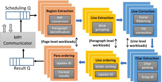
Fig. 12. ITRS cognitive model ... 37
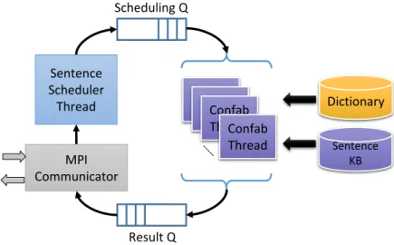
Fig. 13. ITRS pipeline ... 39
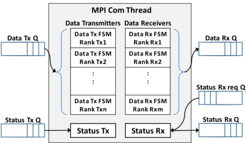
Fig. 14. MPI communication sub-module architecture ... 40
Fig. 15. Flow Control Protocol. (a) Receiver is ready (b) receiver is busy ... 43
Fig. 16. Communication protocol state machines ... 44
Fig. 17. Image processing pipeline ... 45
Fig. 18. Angle computation ... 48
Fig. 19. Tilt correction ... 48
Fig. 20. Intermediate results during image processing ... 51
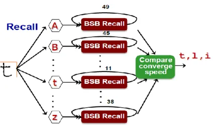
Fig. 21. Candidates are selected based on speed of convergence ... 52
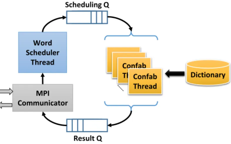
Fig. 22. Word confabulation architecture ... 53
Fig. 23. Trie data structure ... 54
Fig. 24 . Sentence confabulation architecture ... 58
Fig. 25. Micro pipeline performance (a) Image processing, (b) BSB, (c) word confabulation, (d) Sentence confabulation ... 60
Fig. 26. (a) & (b) Accelerator sharing (c) Results demonstrating macro pipelining effect ... 61
Fig. 27. Dynamic load balancing (a) STG, (b) Results ... 62
ix
Fig. 31. Generic neuron model... 67
Fig. 32. Range modifier behavior ... 68
Fig. 33. Winner take all circuit ... 70
Fig. 34. SpNSim architecture ... 74
Fig. 35. Simulation engine control flow ... 77
Fig. 36. Network structure (50x9x9) ... 83
Fig. 37. Nine 5x5 extracted features and corresponding filter responses from our SNN and CRBM ... 84
Fig. 38. 3D NW visualization of 9 feature learning of 5x5 kernel ... 84
Fig. 39. Sentence confabulation network ... 85
Fig. 40. Confabulation results raster plot ... 86
Fig. 41. Efficient winner-take-all circuit ... 90
Fig. 42. Bistable 6-T random number generator design. ... 92
Fig. 43. Dataflow graph for pipelined recall and learning ... 94
Fig. 44. Neuron datapath ... 96
Fig. 45. Network structure for (a) training and (b) testing ... 97
Fig. 46. Confabulation results raster plot ... 100
Fig. 47. Normalized winner-take-all NW ... 104
Fig. 48. Reference network results ... 107
Fig. 49. TrueNorth core fabric ... 108
Fig. 50. Corelet programming environment ... 109
Fig. 51. Design flow ... 109
Fig. 52. Comparing reference network and shadow network ... 110
Fig. 53. SpNSim 3D NW visualization a) Reference NW with Bayesian neurons b) TrueNorth equivalent shadow NW ... 111
Fig. 54. Crossbar connections for lexicon 1 ... 113
Fig. 55. Core and neuron allocation ... 115
Fig. 56. Design Environment ... 117
Fig. 57. TrueNorth sentence results ... 118
x
L
IST OF
T
ABLES
TABLE I. Simulation results comparison ... 34
TABLE II. Validation results ... 62
TABLE III. Classification results ... 84
1
I
NTRODUCTION
The brain has a very efficient and hierarchical architecture to process information [1]. It performs inference and decision-making tasks based on pattern matching and sensory association in the context of learned knowledge, which is the most important step towards cognition. With this motivation, the paradigm of brain inspired computing called neuromorphic computing has gained lot of attention recently. This emerging field of computing is offering a possible pathway for approaching the brain’s computing performance and energy efficiency for cognitive
applications such as pattern recognition, speech understanding, natural language processing etc. Currently more and more complex problems are being attacked using machine intelligence and deep learning concepts which fall under this paradigm. They are being adopted for Industrial applications and in research environment for solving problems which are very hard to articulate as it requires intuitive reasoning along with analytical abilities. Many strides in this field have been made from the inspiration of how the brain solves very complex problems using insights from well-established statistical analysis methodologies. These brain-inspired computing models have three main aspects to it; 1) the model itself which performs inference based predictions, 2) parameters used by the model to enable inference and decision making and 3) training the parameters for tuning the model to make better predictions. The ability of the model to learn is critical because of the vast parameter space one must explore, which is impossible to handle through the traditional programming approach. There are two main components which are the driving force behind these kinds of models. Firstly, large amounts of data and secondly, access to large amounts of compute resources to process it.
in machine intelligence has entered a new era. Meanwhile, modern computing systems are increasingly becoming more heterogeneous. This is due to a wide variety of computing architectures and accelerators such as multi-core CPU, GPU, FPGA, etc. being used. There are many questions which must be addressed for efficient utilization of these resources; how to harness the computing power and storage capacity of modern HPC clusters and convert it to useful computations that assist or even surpass the human cognition process? Will the performance of current neuromorphic computing models scale as the hardware resource increases? What is the bottleneck of current HPC architectures when applied to cognitive computing and how can this be addressed by future computing tools? This work makes a
preliminary effort in answering these questions. We propose a framework to implement complex applications as pipelined distributed applications which are capable of seamless scaling over heterogeneous cluster resources. It is also capable of distributed flow control and dynamic task dependency aware scheduling. Next, we address the problem of efficient resource allocation for such complex systems. We use a complex neuromorphic application, Intelligent Text
Recognition System (ITRS) [2], as a case study to validate the framework and discuss the major advances along different modalities. The background of such a system along with key algorithms will be discussed. Insights into designing modular pipeline stages for complex applications which scale with the available compute resources is provided. We do a comparative analysis of our framework with existing solution for demonstrating the effectiveness of the proposed approach.
On the flip side, the exponential growth of data over the past decade has generated a need for higher processing capability with low energy consumption and ease of scalability. Limitation of the Von Neumann architecture and barriers such as memory capacity, power density etc. in the CMOS technology are being highly tested to meet today’s requirements and also to fulfill
Moore’s predictions. These limitations have motivated novel research efforts in bio-inspired computing, which imitates the structure and function of the brain, the computing engine that is able to process massive amounts of real-time information with less than 20 Watts of power consumption [3]. The processing capability of brain comes from the collective processing abilities of simple processing components i.e., neurons. Interconnected neurons form the basis of a neural network. The ability of neural networks to perform pattern recognition, classification and associative memory, is essential to applications such as character recognition, speech recognition, sensor networks, decision making etc. [4] [5] [6] [7] [8]. SNNs, which use spikes as the basis for communication, are the third generation of neural networks inspired by the biological neuron models [9].
The SNN has the potential to reach very low energy dissipation since each neuron works asynchronously in an event-driven manner. Moreover, fully distributed Spike Timing Dependent Plasticity (STDP) learning [10] can be achieved on SNNs, which updates synaptic weight based only on local information of individual neuron. The emerging field of stochastic SNN that generates spikes as a stochastic process is not only more biologically plausible [11] but also enhances unsupervised learning and decision making [12] [13]. It further increases the fault tolerance and noise (delay) resilience of the SNN system since the results no longer depend on the information carried by individual spikes but the statistics of a group of spikes. With this
inspiration a focused effort is made to present a high-performance SNN simulation framework for developing spiking neuron models and simulation of large-scale SNNs. For efficient and native implementation, digital hardware is proposed for SNN implementation. Finally, a methodology is presented for modelling probabilistic graphical model used in ITRS as SNN is presented, which is realized on off-the-shelf neurosynaptic processor for ultra-low power and
real-time evaluation of the neural network.
1.1
CONTRIBUTIONS
To address the challenges of implementing efficient brain inspired systems different
approaches have been adopted spanning system level design decisions to low level optimizations. The primary contributions of this work are listed below
1. A Scalable Linear Pipeline (SLP) framework is proposed which integrates the
optimization techniques for node level system design and cluster level distributed system design for a holistic approach using existing computing technologies.
2. The concept of scalability of a pipeline is introduced. Each stage is made modular with uniform communication architecture for flexibility of mixed module designs which allow for maximum available resource utilization without the need for expensive application redesign for heterogeneous clusters.
3. Asynchronous pipeline concepts are introduced for such a scalable architecture which enables out-of-order computation, hence minimizing idle time i.e. increased throughput. 4. Novel structure based runtime scheduling is introduced for achieving maximum
performance for asynchronous workload processing with varying module latencies while respecting the data dependencies.
5. For achieving best possible throughput, a set of algorithms are proposed to suggest the mapping of software modules to various hardware resources available on a
heterogeneous cluster.
6. For a more efficient and biologically plausible brain inspired implementation, several spiking neuron models are proposed which are capable of distributed on-line learning.
7. An efficient and high-performance spiking neural network simulator architecture is put forward for large-scale SNN simulation involving mixed neuron models and different learning rules.
8. A digital spiking neuron hardware design is proposed which is capable of online learning for a comprehensive take on SNN implementations. The architecture is pipelined to compute inference and learning task with approximately same throughput compared to existing digital spiking neuron model implementations including those which don’t implement in hardware learning.
9. Finally a streamlined approach is presented to map a probabilistic inference model as a spiking neural network on existing off-the-shelf neurosynaptic processor
2
S
CALABLE
L
INEAR
P
IPELINE
F
RAMEWORK
Today increasingly complex applications are being moved from the end user to the cloud infrastructure [14] [15], due to the cost advantage and ease of access to large amounts of computing resources. This shift has positively impacted the field of research, scientific computing, big data, large scale consumer applications, complex system simulations,
neuromorphic computing, financial modeling etc. The key enablers for this shift are the reducing cost of high performance computing (HPC) resources and the ability to handle large amounts of data [16]. Distributed data storage and management techniques have become very popular to sieve through large amounts of data efficiently [17] [18]. Tremendous technological
advancements are being made in terms of computing accelerators, resulting in the rapidly increasing popularity of heterogeneous clusters. Since these clusters include processors with different basic architectures, they provide unique performance and cost tradeoffs for different types of workloads. To achieve peak performance, software running on heterogeneous cluster needs to be designed carefully to provide enough flexibility to explore its diversity. With these developments in HPC technologies, the design and development of high impact, complex applications, especially in the field of machine intelligence have entered a new era. Since these clusters include processors with different basic architectures, they provide unique performance and cost tradeoffs for different types of workloads. To achieve peak performance, software running on heterogeneous cluster needs to be designed carefully to provide enough flexibility to explore its diversity.
These applications are designed as linear pipelines to maximize their throughput as they process huge amounts of requests in a streaming manner while requiring access to large amounts
of data. They have the ability to hide the overhead of managing communication, processing and synchronization which are very beneficial for HPC paradigm [19]. Significant research has been made in modeling such applications especially in the context of large-scale platforms. There are many challenges including the design of applications, identifying different stages of the pipeline, identifying a suitable pipelining model, data partitioning, parallelizing, mapping of pipeline stages to different resources etc. Traditionally Linear pipeline models are preferred due to their
simplicity in design and implementation. For streaming applications, all stages of the pipeline must be active and processing requests hence requiring more resources compared to non-streaming applications where interval based resource allocation is a standard. These linear pipeline models are limited in terms of their scalability. To scale these models, it requires a fresh look at how the stages can be re-decomposed to improve the performance. In this work, we propose a Scalable Linear Pipeline (SLP) framework which overcomes these limitations and affords seamless scalability over a heterogeneous cluster while performing dynamic distributed load balancing, distributed flow control along with data dependency aware scheduling. In a heterogeneous cluster a stage can be mapped to run on only a limited number of nodes, making the problem of mapping the pipeline harder. It is a non-trivial task to determine a mapping for such a highly-constrained model as in this model we allow simultaneous compute resource sharing for stream processing which is more desirable in the real-world applications.
We build the SLP framework using principles of traditional lineal pipeline model. The task dependencies spanning across different stages is modelled as a dependency graph and how their behavior scales with the increasing number of resources is outlined. The SLP allows automatic load balancing and self-scheduling. These capabilities are explained using the dependency graph and a simple analytical performance estimation model is presented. The SLP also allows flexible
resource utilization. The algorithm for mapping the SLP to available resources in a heterogeneous cluster is discussed.
Distributed systems are widely used and have been extensively studied. Different kinds of distributed pipeline based architectures are proposed. A state based distributed pipeline
framework is presented in [20]. Here the compute nodes are separated from the pipeline control. Instead of message passing the state objects are passed which encapsulate the data. The load balancing is achieved through producer/consumer relationship i.e. processing happens asynchronously. However, there is an extra overhead in creating and decoding state objects at every stage apart from data processing. A distributed pipeline processing architecture composed of flow-models, called meta-pipeline is proposed for general-purpose computation [21]. The architecture is suitable for stream based processing. This requires input and output streams along with the parameters for every flow-model. These details and other properties are encapsulated in XML. This kind of modularization enables distributed task based execution. Though this system is distributed it requires centralized management to assign and load flow-models. Fully utilizing the performance of heterogeneous resources is a challenging task. Design methodology for executing applications on heterogeneous platforms, which are specified as synchronous dataflow (SDF) graphs is proposed in [22]. The authors try to maximize the end-to-end throughput of an application developed in OpenCL by modeling it using SDF graph. Data-intensive workflow optimization is presented in [23] which uses task graph partitioning to improve the performance of streaming applications on heterogeneous systems. By minimizing the data movement between partitions, they reduce the latency and increase the overall throughput, however they allow task duplication across partitions. This method is not suitable for applications which have dynamic task dependencies.
Mapping such pipelined applications to compute resources is a non-trivial task. The work presented in [24] discuss the theoretical aspects of a linear pipeline with computation and communication overlap. They present models for interval based resource mapping for homogeneous and heterogeneous platforms. The ELPC model presented in [25] discusses mapping of linear pipeline models over a wide area network. They present a dynamic
programming approach to solve the mapping problem. A similar approach is demonstrated in [26] with a focus on visualization pipeline. In the above works the mapping is done with interval based resource sharing. This introduces additional complexities on optimizing buffer sizes which is studied in the work presented in [27]. These approaches are not very scalable as the pipeline design has to re-worked to improve the performance. These pipeline models are developed for distributed applications. They also don’t address the problem of task scheduling for complex workloads which is partly because their models don’t scale easily hence having very simple first come first serve scheduling. A cuckoo search based scheduler for mapping of workflow tasks on heterogeneous cloud resources is presented in [28].
Clustering Method based Task Dependency resolution scheme is introduced in [29] to handle today’s complex data dependent task scheduling in distributed application environments. In this task clustering methodology, they merge fined-grained tasks into coarse-grained jobs. Hence, with clustering they try to reduce execution overhead and to improve the computational granularity on distributed resources. This approach, requires the detailed knowledge of tasks which differ significantly for different applications and also needs a centralized analysis to determine the scheduling behavior. Ke Wang et al. [30] present a locality aware load balancing scheme for data-intensive workloads many-task computing models. This is a fully distributed task scheduling architecture however; this approach requires full connection among compute nodes
which is not always ideal. A k-means algorithm based initial data placement strategy [31] is introduced to have optimized task scheduling for data intensive workloads for distributed applications.
In contrast to the aforementioned related works, the goal of our work is to show how complex application with various processing requirements can be converted to scalable, distributed applications even for data intensive workloads. The research community has been focusing on different aspects of pipeline processing and strategies for scaling applications in distributed environments as different problems. This is the first work to our knowledge where we introduce the concept of scaling of pipelined application models over distributed resources. We also
introduce a distributed scheduling strategy for such implementations which enables dynamic load balancing and out-of-order execution for higher hardware resource utilization. Compared to a traditional linear pipeline optimized using the Efficient Linear Pipeline Configuration (ELPC) [25], the SLP and our proposed resource mapping algorithm achieve the resource utilization efficiency, which was not possible before. To validate our performance estimation model and to demonstrate the potential of the SLP, we implement a neuromorphic application called Intelligent Text Recognition System, as a case study. Details of pipeline construction, management,
scheduling and inter-stage communication are discussed. The experimental results show that our performance estimation model achieves 96% accuracy compared to the measured results, and our resource mapping algorithm improves resource utilization and is capable of providing linear scaling where ELPC failed to address these concepts.
2.1
PIPELINE MODEL
considered during the design phase. Latency of such applications play an important role however, it is not critical while determining the sustained throughput. Large applications, requiring heavy computation while needing access to large databases are typically implemented as deep pipelines. Pipelines are efficient for streaming applications as they have the ability to hide latencies across various stages, while trying to optimize for maximum resource utilization. In general, complex applications are looked as a linear sequence of distinct stages. Each stage in a linear pipeline performs a task in-order, hence they are referred to as first-in-first-out systems.
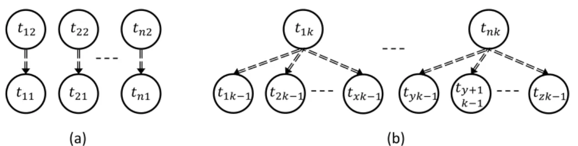
Various graph based models have been used to capture task dependicies. A workflow graph representing linear task dependencies which can be resolved in-order fashion is shown in Fig. 1. Each node in this graph represents a computation task and the directed edge represents the data dependency. For example, 𝑡2 depends on 𝑡1 and so on until the final task 𝑡𝑥 which depends on its
previous task 𝑡𝑥−1. It is important to note that the task dependency is known at design time and it specifies the task execution order. We assume that ASAP scheduling is adopted, which will start the execution of a computing task as soon as all of its inputs are ready and the computing resource is available. If multiple tasks are ready for execution, then the earliest one will be picked.Fig. 1. Each node in this graph represents a computation task and the directed edge represents the data dependency. For example, 𝑡2 depends on 𝑡1 and so on until the final task 𝑡𝑥
which depends on its previous task 𝑡𝑥−1. It is important to note that the task dependency is known at design time and it specifies the task execution order. We assume that ASAP scheduling is adopted, which will start the execution of a computing task as soon as all of its inputs are ready and the computing resource is available. If multiple tasks are ready for execution, then the earliest
Fig. 1. Typical task dependencies of a linear pipeline
𝑡2 𝑡1
one will be picked.
The above linear dependency directly corresponds to a Linear Pipeline (LP) model. Fig. 2 shows a generic block diagram of such a linear pipeline. It has 𝑙 stages. The output 𝑊𝑘 of any stage 𝑚𝑘 where 1 ≤ 𝑘 ≤ 𝑙 is considered as the workload for subsequent stage 𝑚𝑘+1, here 𝑊0 is the input to the pipeline and 𝑊𝑙 is the final output of the pipeline. Each workload represents a
single task for the next stage. Each stage of the pipeline can resolve one task or a sequence of consecutive tasks in the workflow graph. After modeling the pipeline, we map each stage to a computing resource. To achieve the highest parallelism and maximum resource utilization, it is desirable to have similar latency in each stage hence no computing resource is idle during the processing.
We focus our attention towards streaming pipelines as they are more practical in processing large datasets by taking advantage of concurrent stages. Especially when it is required to look up large distributed databases which is common in today’s applications such as; neuromorphic applications, business intelligence, big data, machine learning, deep learning etc. The only way to scale such pipelines is to break the tasks at a finer grain and make the pipeline deeper, i.e. add more stages to increase the effective parallelism. However, this is limited by the granularity of hardware computing resources and the parallelism within a computing task.
A traditional linear pipeline as shown in Fig. 2 is primarily a first-in-first out system which doesn’t scale efficiently. Making the pipeline deep is the only way of scaling which has a significant overhead in terms of remodeling the tasks and redesigning the computing stages to
Fig. 2. Linear pipeline model
𝑚1 𝑚2 𝑚𝑙
𝑊0 𝑊1 𝑊2 𝑊𝑙−1 𝑊𝑙
scale such pipelines. To overcome the pipeline scaling issue, we propose a Scalable Linear Pipeline (SLP) framework. The SLP looks at the application at the cluster level and treats it as a macro pipeline. To achieve best performance every module must be efficient enough to keep this macro pipeline busy as much as possible. To achieve this goal, we treat each module as a micro pipeline. Each stage is treated as a pipeline for achieving higher throughput but this is not a binding requirement by the framework. We employ a modular approach to enable scaling not only along the number of stages but we scale at every stage, hence resulting in wider pipeline. A typical SLP is shown in Fig. 3.
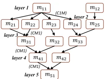
In contrast with a LP, SLP consists of consecutive layers composing a linear pipeline as each layer consists of multiple parallel instances of a stage. Therefore, SLP consists of 𝑙 layers. Each layer 𝑘, 1 ≤ 𝑘 ≤ 𝑙 is a set of parallel stage instances 𝑚𝑘𝑖 called as modules, where 𝑖 ≥ 1 is an
arbitrary number based on the scaling of the 𝑘𝑡ℎ layer. Multiple independent tasks are grouped as workload to minimize traffic between modules and reduce the compute resource idle time at the destination module. The result 𝑊𝑘𝑖 of any module of a layer 𝑙 is considered as the workload for subsequent layer 𝑙 + 1, here 𝑊0𝑖 are the input workloads to the pipeline and 𝑊𝑙 is the final output of the pipeline.
In SLP, tasks in the workflow graph are partitioned such that there are no data dependencies across workloads of the same layer. The modules in the same layer operates asynchronously.
Fig. 3. Scalable linear pipeline model
𝑊𝑙 𝑊𝑙−11 𝑊𝑙−1𝑙 𝑙1 𝑙𝑙 𝑊21 𝑊2𝑙 𝑚21 𝑊11 𝑊1𝑙 21 2𝑙 𝑚11 𝑊01 𝑊0𝑙 11 1𝑙 𝑚𝑙1
There is no guarantee of the order of the task completions. This will not cause problem because the task precedence constraints are ensured by the structure of the pipeline and the ASAP scheduling of resolved tasks. Due to scaling of a layer a task can have dependencies from different modules of previous layer. Any unresolved task is buffered to enable computation of resolved tasks in out-of-order manner. Even with such task dependency, this model is a linear pipeline as the dependencies are between consecutive layers. The last layer of SLP has only one instance, which collects and reorder the out-of-order completed tasks.
Each module can have a variety of design requirements based on the application hence, it is not practical to build a model which suits all the design decisions of distributed applications. Instead we outline few strategies which are ideal for SLP based implementation. An input task can be further parallelized to sub tasks and scheduled to thread pools or multiple whole tasks can be scheduled to thread pools for computation on a CPU based architecture. The computation can be vectorized or can be accelerated and optimized based on the hardware platform requirements. The key idea behind these suggestions is to keep the hardware resources busy as long as possible while maintaining out-of-order computation which perform task resolution based scheduling. For these micro pipelines to work together a common communication interface which runs
independently and in parallel to computation is needed to make the system design modular so as to scale seamlessly. Therefore, SLP is a pipeline of pipelines working asynchronously.
The proposed SLP is flexible as it is agnostic to the nature of computation that happens within an instance of a stage as long as the input and output workloads are of same type as in that layer. Therefore, the model supports modular design for implementing the pipeline as modules in a layer can be implement on different hardware platforms and technologies with different latencies. A typical task dependency graph for SLP is shown in Fig. 4 for three consecutive layers. Here
task 𝑡1𝑘 of layer 𝑘 has dependence on a set of tasks 𝑡1𝑘−1 up to 𝑡𝑥𝑘−1 of previous layer 𝑘 − 1. From the figure, hierarchical task dependency is evident.
Task data dependencies are application and data specific. In some applications where bottom up processing is used, the output of multiple computing tasks at fine granularity will be
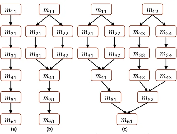
assembled as one workload to trigger higher level processing. In other applications where top down processing flow is used, the output of one upper level computing task will trigger multiple lower level computing tasks. Although both are interesting scenarios in the SLP optimization, the latter is more challenging in the SLP, which performs out-of-order-execution, because it consists of tasks with multiple dependencies. The number of upper or lower level tasks and their relations are often not fixed, but rather data driven. To support out-of-order computation we allow breaking linear tasks to fine grained sub-tasks when compared to LP model. This procedure creates dependency as the actual task is resolved only when the sub-tasks are resolved. The number of sub-tasks is dependent on the size of the actual task which is dynamic. These sub-tasks are treated as independent tasks in SLP, which are processed by employing fork and converge strategy. As the tasks across the layers converge downstream their dependencies get resolved and the processing gets done hierarchically. Therefore, actual task dependence graph cannot be known at design time. The first layer forks the tasks, the middle layers converge hierarchically to resolve the dependencies and the last layer is to re-order the out-of-order resolved tasks.
Fig. 4. Typical task dependencies of a scalable linear pipeline 𝑡1𝑘−1 𝑡1𝑘 𝑡2𝑘−1 𝑡𝑥𝑘−1 𝑡 𝑘−1 𝑡 𝑘 𝑡 +1 𝑘−1 𝑡 𝑘−1 𝑡1𝑘+1
Therefore, SLP requires a minimum of 3 layers to support the fork and converge design methodology. The number of upstream layer tasks required to resolve one task in the current layer cannot be known at design time. Such information is only available during runtime.
However, the general fork and converge structure is known at design time. Using this knowledge structure based runtime scheduler is proposed to resolve these dynamic task dependencies. We discuss this in section 2.5.
In the proposed design methodology, the communication happens asynchronously and in parallel to computation. Therefore, the communication latency is hidden. Let 𝐿𝑠𝑐 represent the link delay between a given pair of adjacent layer modules (𝑚𝑠, 𝑚𝑐) where subscript 𝑠 stands for source and 𝑐 stands for consumer. Since the latency is hidden 𝐿𝑠𝑐 is not a critical parameter in our model. For SLP to guarantee deadlock free operation the input of every module must have input buffers large enough to accommodate partial results from previous layers till the task of that layer is resolved. It must have output buffers as well to temporarily store the results from the micro pipeline till the results can be forwarded to the next downstream module. If the output buffer is full then it stalls the micro pipeline, till there is room to store new results. However, it is straight forward to compute the minimum size of input and output buffers of a module by accounting for the variance in the rate of messages received and the rate of messages processed. In this work, we target a computing cluster, more specifically a heterogeneous cluster instead of a wide area network of computing resources. Therefore, the latencies 𝐿𝑠𝑐 are small. Our model can be easily
extended to a wide area network scenario with larger input and output buffers to account for the variability of message arrival rates and link latencies.
2.2
DYNAMIC DATA DEPENDENCY
To accommodate scaling at layer level, the modularization strategy was based on breaking complex tasks into multilevel data dependencies and creating large number of small independent workloads which can be processed parallelly by different modules in a layer. This results in dynamic data dependencies which need to be resolved in real time. The first layer creates small independent tasks which are forked to the next layer hence, there is one-to-one task dependency with the second layer as shown in Fig. 5(a). The dependency is one-to-one because bottom-up approach is used and the first layer created the leaf tasks which must be now processed in the next layer.
All other consecutive layers have convergent task dependence as shown in Fig. 5(b). A workload is a group of tasks which is transmitted as messages from one module to other across consecutive layers over point to point links. Since all tasks in a layer are independent, all tasks with in any given workload are mutually exclusive. However, those tasks have dependencies across layers. Depending on the resources available and the input these tasks complete asynchronously. Task 𝑡𝑥 at the 𝑘𝑡ℎ layer is resolved if the set of dependent tasks Γ
𝑥𝑘−1 from the
previous layer in the graph are computed which is denoted as
𝑋(𝑡𝑥𝑘) =∧∀𝑡𝑖∈Γ𝑥𝑘 (𝑋(𝑡𝑖))
(a) (b)
Fig. 5. (a) Task dependency between 1st and 2nd layer (b) Task dependence between
consecutive layers except 1st and 2nd layer 𝑡11 𝑡12 𝑡21 𝑡22 𝑡 1 𝑡 2 𝑡1𝑘−1 𝑡1𝑘 𝑡2𝑘−1 𝑡𝑥𝑘−1 𝑡 𝑘−1 𝑡 𝑘 𝑡 +1 𝑘−1 𝑡 𝑘−1
The results of the subset of tasks belonging to Γ𝑥𝑘−1 which are not yet resolved must be buffered at the input of every module until 𝑋(𝑡𝑥𝑘) is resolved. Once 𝑋(𝑡𝑥𝑘) is resolved, task 𝑡𝑥𝑘
is scheduled for computation. The rate at which 𝑋(𝑡𝑥𝑘) is resolved depends on the input and the
compute resources available, therefore it is critical to have multiple such tasks queued up to increase resource utilization. This condition can be met by having large number of tasks in the workloads and having multiple redundant paths of execution in the scaled pipeline which is determined by the width of the pipeline at that layer.
To support such task resolution in a de-centralized manner we apply constraints on the connectivity pattern among modules between every consecutive layer. We use point-to-point connectivity between modules of consecutive layers to keep the data flow de-centralized. Two types of connectivity patterns are used to support the fork and converge model described earlier as shown in Fig. 6.
Fig. 6(a) shows the connectivity constraints between the first two layers of the pipeline, it has one-to-many connectivity (C1M) pattern. Fig. 6(b) shows the connectivity constraints between all consecutive layers except 1st and 2nd layer. This pattern has many-to-one connectivity (CM1). For
the case of C1M the module 𝑚1𝑥 breaks up its workload into small tasks and schedules it to one of its out-going paths thereby performing a fork operation. CM1 on the other hand performs the converge operation by reducing the results from several upstream tasks. Since CM1 is present
(a) (b)
Fig. 6. (a) Single fan-in, multi fan-out connectivity (b) Multi fan-in, single fan-out connectivity
𝑚1𝑥
𝑚21 𝑚22 𝑚2
𝑚𝑘1 𝑚𝑘2 𝑚𝑘𝑥
between many layers, the reduction happens hierarchically. Therefore, the connectivity
constraints which help in determining the number of source and consumer modules is expressed as
C1M constraint: |𝑚𝑠| ≤ |𝑚𝑐|
CM1 constraint: |𝑚𝑠| ≥ |𝑚𝑐|
We try to match the performance of each layer by managing the level of parallelism in each layer. The the number of modules required in each layer is determined to achieve the required performance, we refer to this as scaling. After determining the scaling of each layer, these modules are interconnected based on the connectivity constraints. The resulting pipeline graph is called as System Topology Graph (STG). Fig. 7 shows an example of a typical STG for the SLP. This example has 5 layers with 2,5,3,2,1 scaling in layers 1 through 5 respectively. It is interesting to note that SLP is a super-model of LP model. If we restrict one module per layer and restrict that each workload is one task then SLP reduces to a LP model.
Fig. 7. A typical system topology graph
𝑚11 𝑚21 𝑚22 𝑚2 𝑚 1 𝑚 2 𝑚 1 𝑚12 𝑚2 𝑚2 layer 1 layer 2 layer 3 layer 4 (C1M) (CM1) (CM1) 𝑚 𝑚 2 𝑚 1 (CM1) layer 5
2.3
PERFORMANCE MODEL OF SLP
Every module of the 𝑘𝑡ℎ layer, 𝑚 ∈ 𝑚
𝑘1, 𝑚𝑘2, 𝑚𝑘 , … , 𝑚𝑘𝑖 can run with different
configurations resulting in different throughput ∈ 𝑘1, 𝑘2, 𝑘 , … , 𝑘𝑖. Those configurations include the number of threads in the software implementation, the assignment of hardware platform, or other algorithm based settings. Different binaries can also be developed to run the same module on different hardware architecture. These binaries are individual processes represented as 𝑝 ∈ 𝑝1, 𝑝2, 𝑝 , … , 𝑝𝑢 where 𝑢 is the maximum number of processes for any
given module 𝑚. Therefore, 𝑐 ∈ 𝑐1, 𝑐2, 𝑐 , … , 𝑐 represent configurations where, 𝑛 is the maximum number of unique set of process-parameters associated with each given process 𝑝 of a module 𝑚. In other words, a module 𝑚 can be realized by any of 𝑐1 to 𝑐 configurations. Where
each configuration represents a process binary for a given hardware architecture along with the associated parameters. Each layer can run a mixture of these configurations hence SLP has a large design space.
It is a common practice to model the processing performance of different hardware nodes used in the system to be normalized across performance of different modules. This abstraction encapsulates the processing speed, memory, bus speed etc. and makes mapping algorithms simpler however, this adds an approximation to the model. Instead of modeling the system using normalized processing requirements for modules and the available hardware resources, we perform dry runs to collect empirical data for reliable performance modeling. However, this is not a limiting factor, as the same model can be used with normalized representation of performance requirements. For every server 𝑠 ∈ 𝑠1, 𝑠2, 𝑠 , … , 𝑠𝑟 with 𝑟 nodes in the heterogeneous cluster,
let 𝑇𝑚𝑎𝑥,𝑠 denote the number of logical cores in 𝑠, and 𝑀𝑚𝑎𝑥,𝑠its peak memory bandwidth. This gives us the upper limit of the supported compute and memory bandwidth capacity for every
server 𝑠.
Next, we determine the CPU level thread concurrency 𝑇 and the memory bandwidth 𝑀
needed to run every configuration 𝑐 of each module along with its run time 𝜏. It is necessary to measure the CPU level concurrency as each module configuration consists of threads performing different tasks which are not always concurrent, this way we obtain the actual impact of the configuration on specific compute resource. To enable this data collection, each process along with its set of parameters must be analyzed independently i.e. ∀𝑐 ∈ 𝑚. The value of 𝜏 recorded is the run time achievable for the given configuration 𝑐. The value of 𝜏 is normalized to the unit task the end-to-end pipeline is processing to get per unit work of runtime. 𝑇 and 𝑀 are not normalized as they represent the steady state requirements to run a configuration. Rate is computed as = 1/𝜏 which represents the number of unit work processed per second for every 𝑐 ∈ 𝑚.
For SLP to run at maximum performance all modules must be processing at maximum capacity. This is possible when every module is receiving tasks at maximum input rate. Therefore, to determine the performance of such a pipeline we measure the performance of individual modules in a standalone manner for maximum input rate. Using the standalone
performance as building blocks, we determine the SLP performance. In practice, it is not practical to assume that all the modules have same performance. The performance of SLP is determined by the layer with least throughput, i.e. max runtime. Therefore, we model the throughput 𝑃 of SLP as
𝑃 = 𝑚𝑖𝑛𝑘=1 𝑡𝑜 𝑙(∑𝑖=|𝑚𝑘| 𝑘𝑖)
Mapping hardware resources to run different modules and to determine the STG for such mapping while optimizing the end-to-end throughput is a non-trivial task. We provide the solution for this challenge in section 2.4 based on the performance model discussed here.
2.4
RESOURCE MAPPING FOR MAXIMUM THROUGHPUT
To achieve high performance, all pipeline stages should have the same throughput. However, the workloads of different layers differ significantly. A layer with heavy load should be able to grab more computing resources and scale accordingly. Each software module which runs on a hardware node can employ multi-threading or any hardware platform specific acceleration and optimization to achieve maximum efficiency possible. The performance of a module
(configurations 𝑐) and the number of modules in a layer are parameters that are determined to keep a balanced pipeline. To allocate more resources to a particular layer, we simply need to instantiate more modules or use different configuration of a module of that layer. In a
heterogeneous system, their selection not only depend on the layer a module belongs to but also the hardware that the modules and its configurations that can run on it.
The goal of resource mapping is to find the best SLP structure and a mapping between SLP modules and hardware computing resources to achieve optimum throughput. During this
procedure, we add or remove SLP modules to balance the throughput among layers, therefore the structure of SLP and the mapping scheme evolve simultaneously. Please note that in a
heterogeneous system, maximum resource utilization does not necessary mean maximum throughput.
Resource mapping for maximum performance is a hard combinatorial problem. Our heuristic algorithm consists of two major steps. First, we find a minimum feasible solution (MFS) such that one module from every layer is assigned a compute resource. Then we improve the MFS by allocating additional modules to available compute resources to eliminate bottlenecks and achieve a desired throughput. The throughput of every module and end-to-end throughput of the pipeline is measured in terms of number of unit-work processed per second.
Many constrained resource matching problems are solved using dynamic programming, which has pseudo-polynomial time complexity. To apply dynamic programming, we must be able to construct the optimal solution of the problem based on the optimal solution of its sub-problems. This requires the solution space to be discretized resulting in re-use of sub-problem solutions. The work presented in [25] solves a resource mapping problem for a linear pipeline using dynamic programming techniques. They propose an algorithm called Efficient Linear Pipeline Configuration (ELPC) with a constraint that a hardware resource is not concurrently running multiple modules while optimizing for end-to-end throughput. ELPC however allows interval based resource sharing with different modules which is again non-concurrent sharing. In the proposed pipeline model each module has multiple configurations who are candidates for resource mapping to hardware resource which is already mapped with a configuration which has partially utilized that resource. This kind of mapping improves resource utilization efficiency. Therefore, the proposed model is more efficient than ELPC as it tries to utilize the hardware resources to the maximum extent possible. Since SLP allows simultaneous resource sharing, the sub-problems of partial resource allocation can’t be guaranteed to have optimal solution due to fractional allocation of resources. The sub-problem solution can’t guarantee optimal sharing of a resource till all the configurations of not yet visited sub-problems are analyzed. Therefore, we propose a solution based on backtracking methodology.
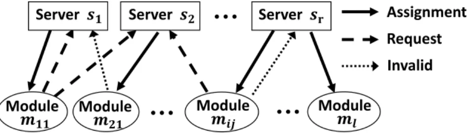
For solving the mapping and throughput optimization problem we make use of a resource allocation graph with some enhancements to keep track of resource sharing, we call this
Simultaneous Resource Allocation Graph (SRAG) as shown in Fig. 8. Every edge represents a configuration 𝑐 of a module 𝑚. A request edge represents a resource allocation request from a module to a hardware resource. The assignment edge represents a mapping between module and
hardware. We introduce another type of edge called invalid edge which is represents a configuration that was deemed infeasible for mapping based on the available resources.
Therefore, to run a module there are a set of associated configurations which can be allocated to hardware resources based on their availability in the cluster. Each configuration has an associated cost in terms of required concurrency, memory bandwidth, number and type of accelerator cards etc.
We now introduce the properties and methods of SRAG. The SRAG is used to keep track of module assignments. It evolves iteratively till a final solution is obtained. Each iteration consists of updating an edge state of SRAG which involve setting an edge type as assignment, request or invalid. A request edge of SRAG is transformed to an assignment edge if the hardware has enough resources available as required by the cost of the edge, if not than this edge is transformed to an invalid edge. Whenever an edge is transformed from request or invalid type to assignment type then the edge-cost amount is deducted from the available resources for that server, indicating the amount of hardware resource used up for this assignment. Inversely, when an edge is
transformed from assignment type to request or invalid type then the edge-cost amount is added back to the available resources of that server, indicating freeing up of hardware resources.
An evolution of SRAG is defined as a set of iterations of SRAG which result in assigning minimum number of modules which results in an increase of overall throughput. After every
Fig. 8. A typical simultaneous resource allocation graph
Assignment Request Invalid Module Module Module Module
evolution of SRAG the corresponding STG is computed. It is important to note that a module can have only one assignment edge associated with it as it can run on only one server at a time. In contrast, STG consists of connections between the modules which represents the actual system topology of the modularized distributed application which runs on the heterogeneous cluster.
2.4.1
M
INIMUMF
EASIBLES
OLUTIONInitial SRAG is created with one modules each for a layer. It also has as many resource vertices as the number of available servers. The SRAG at this point has only request edges, which represent all possible configurations 𝑐 to work with. The MFS algorithm is a recursive function based on backtracking principles. Backtracking performs exhaustive recursion which can be potentially very expensive. For every recursive call, we make a decision-point for getting a feasible assignment and continue further to explore next feasible assignment. If further such assignment is not possible then we backtrack to the decision-point and try other alternatives. In this way, we backtrack only as far as needed. We apply a heuristic by pre-processing the input to the algorithm to reduce the recursion depth for average case.
A list of request edges is made by selecting one edge per module from the request edges belonging to each module. The selected edge has minimum run time among all the request edges of that module. While comparing a tie on run time is broken with the edge having minimum memory bandwidth and a tie on this is further broken with the layer priority of the module. Modules in layer 1 have highest priority and modules of layer 𝑙 have the least priority. This list represents the best possible assignment each module can potentially get. It is logical to map upstream modules before the downstream ones so that potential bottleneck may appear in lower layers hence reducing future optimization effort. For this reason, layer priority is used as a tie breaker. These selected edges are now sorted with the same comparison policy but in descending
order. Therefore, the edge with highest runtime is on top in the sorted edge list. We now make a two-dimensional jagged array (modEdgeLists𝑚𝑒𝑙) with each row containing all the request edges of a module. The order of rows of this array is same as the module order associated with the sorted edge list. The row order represents the possible bottleneck layer hence this module will be mapped first. Each column of a row in 𝑚𝑒𝑙 represents the possible configurations the module represented by that row can have. The elements of every row are sorted in ascending order with the comparison policy mentioned above. From this ordering of 𝑚𝑒𝑙 we can say that; potential bottleneck layer is assigned its best configuration first. Ordering of 𝑚𝑒𝑙 which is the adjacency list of SRAG constitutes the pre-processing of initial conditions to the algorithm.
2.4.2
S
LACKB
ASEDT
OPOLOGYC
REATIONEach module vertex has 3 parameters; input rate slack (IRS), output rate slack (ORS) and
maximum output rate (MOR). MOR is the inverse of compute time of the assigned edge to that
Algorithm 1. Minimum Feasible Solution
FunctionMFS
Input: modEdgeLists 𝑚𝑒𝑙, module index 𝑚𝐼𝑑𝑥
Output: feasible edge assigned for each edge 𝑒 ∈ 𝑚𝑒𝑙[𝑚𝐼𝑑𝑥] do
if e=type Request then
if assignment of 𝑒 is possible then set 𝑒 type ← Assign
edgAssigned ← true if 𝑚𝐼𝑑𝑥 ≠ 𝑙 then
𝑚𝐼𝑑𝑥 ← 𝑚𝐼𝑑𝑥 + 1
if MFS(𝑚𝑒𝑙, 𝑚𝐼𝑑𝑥)=false then set 𝑒 type ← Invalid edgAssigned ← false
𝑚𝐼𝑑𝑥 ← 𝑚𝐼𝑑𝑥 − 1
If edgAssigned = true then break
else
set 𝑒 type ← Invalid if edgAssigned = false then
for each edge 𝑒 ∈ 𝑚𝑒𝑙[𝑚𝐼𝑑𝑥] do set 𝑒 type ← Request
return false return true
module, which is a constant value for a given configuration, i.e. the hardware platform, process and its parameters. These parameters are used to keep track of the rate at which a module can process input and generates output.
We know that the connections between modules can be of type C1M or CM1. Between any two consecutive layers, the modules which generate the output are called Source Modules (SM) and the downstream modules are called Consumer Modules (CM). For the case of C1M
connectivity, the number of possible connections is equal to the number of fan in slots possible which is equal to the number of CMs. On the other hand, for CM1 connectivity the number of connections is equal to number of SMs. Algorithm 2 shows how the connections between processes are made. These connections are made between assigned modules of SRAG hence, generating an STG which will be used to run the application on the heterogeneous cluster. The algorithm uses a max priority queue called sharedConVrtxQ. This queue holds module vertices with a parameterized comparison policy to either compare IRS values of member modules or ORS.
In Algorithm 2, the Clear existing topology mapping step not only removes all module to module connections it initializes the IRS and ORS values to be equal to MOR. When a connection between two processes is made then slack updates are made as follows, where a subscript ‘c’ representing consumer module parameter and subscript ‘s’ representing source module parameter;
if 𝐼𝑅𝑆𝑐 ≥ 𝑂𝑅𝑆𝑠then
𝐼𝑅𝑆𝑐 = 𝐼𝑅𝑆𝑐 − 𝑂𝑅𝑆𝑠 and 𝑂𝑅𝑆𝑠 = 0. On the contrary if 𝐼𝑅𝑆𝑐 < 𝑂𝑅𝑆𝑠then
These module node parameter updates help in keeping track of what is the available slack per module based on the connectivity. This information will be used in the throughput optimization algorithm to determine the bottleneck layer based on the number of modules in that layer and the associated input and output connectivity of modules.
Once the module parameters, IRS and ORS are computed based on the system topology, the
effective output rate (EOR) for every assigned module in the topology and the layer effective output rate (LEOR) is computed for every layer in the topology. EOR for any given module 𝑚 is computed as,
𝐸𝑂𝑅𝑚 = 𝑀𝑂𝑅𝑚− 𝑂𝑅𝑆𝑚
Finally, the LEOR a layer 𝑘 ∈ 𝑙 is computed as,
𝐿𝐸𝑂𝑅𝑘 = ∑𝑚∈𝑣𝑘𝐸𝑂𝑅𝑚 Where 𝑣𝑘 ∈ 𝑣𝑚 for the given layer 𝑘. Algorithm 2. System Topology Creation
Input: modVertices 𝑣𝑚
Output: system topology Clear existing topology mapping srcLyr←first element ∈ 𝑙
for eachconsLyr | consLyr ← ∀ 𝑙 exceptfirst elementdo
if (connectivity type(srcLyr, consLyr) ∈ C1M connectivitythen set sharedConVrtxQ compare policy ←ORS
insert 𝑚 ∈ 𝑣𝑚|𝑚 ∈ srcLyrinsharedConVrtxQ
insert 𝑚 ∈ 𝑣𝑚|𝑚 ∈ consLyrinarrayoneConVrtx
sort oneConVrtx in descending order of IRS else
set sharedConVrtxQ compare policy ←IRS insert 𝑚 ∈ 𝑣𝑚|𝑚 ∈ consLyrinsharedConVrtxQ
insert 𝑚 ∈ 𝑣𝑚|𝑚 ∈ srcLyrinarrayoneConVrtx
sort oneConVrtx in descending order of ORS for eachmodule 𝑚 of oneConVrtx do
if sharedConVrtxQ not empty then
𝑠𝑐𝑚 ← dequeue sharedConVrtxQ
if (connectivity type(srcLyr, consLyr) ∈ C1M connectivitythen make connection from 𝑠𝑐𝑚 to 𝑚
ifORS of 𝑠𝑐𝑚 ≠ 0 then
insert 𝑠𝑐𝑚 insharedConVrtxQ else
make connection from 𝑚 to 𝑠𝑐𝑚
if IRS of 𝑠𝑐𝑚 ≠ 0 then
2.4.3
T
HROUGHPUTO
PTIMIZATIONThe process of throughput optimization involves identifying bottlenecks and removing them layer after layer. If a MFS exists then, STG must be analyzed for bottlenecks. A bottleneck occurs if a layer with higher priority has higher throughput compared to its immediate layer with lower priority. The end-to-end throughput 𝑃 of the pipeline and the bottleneck 𝐵𝐿 layer is
𝑃 = 𝑚𝑖𝑛𝑘=1 𝑡𝑜 𝑙(𝐿𝐸𝑂𝑅𝑘 )
𝐵𝐿 = 𝑘 ∈ 𝑃
While comparing 𝐿𝐸𝑂𝑅 values, the layer priority is used as a tie breaker. Therefore, if multiple layers have same output rate then the upstream layer is correctly identified as bottleneck layer, we call this operation as getBottleneckLyr. 𝐵𝐿 may not be the effective bottleneck layer when we are trying to scale the number of modules in a layer as we need to satisfy two kinds of constraints; slack and connectivity constraints at the bottleneck layer. Based on these constraints the effective bottleneck layer (ebl) is determined. The slack constraints (𝑆𝐿𝐶) are defined as
𝑆𝐿𝐶 = {∑𝑚∈𝑣 𝑂𝑅𝑆𝑚 = 0 , 𝑖𝑓 𝐵𝐿 = 1 ∑𝑚∈𝑣𝐵𝐿+ 𝐼𝑅𝑆𝑚≠ 0, 𝑖𝑓 1 < 𝐵𝐿 < 𝑙
If the bottleneck is at the first layer then the aggregate 𝑂𝑅𝑆 must be saturated to warrant a scaling of this layer. On the other hand, when the SMs have saturated the input capacity of the CMs for 1 < 𝐵𝐿 < 𝑙 while SMs belong to bottleneck layer then, scaling SMs will have no increase of overall throughput. Therefore, ebl would be the layer of CMs and this layer must be scaled. After ebl is determined the layers that must be scaled to resolve the bottleneck is
determined based on the C1M and CM1 constraints. A list of these layers is called as affected layers (AL). The expression for connectivity constraints (𝐶𝑂𝐶) used in the algorithm to determine
𝐶𝑂𝐶 = {
|𝑚1| + 1 ≤ |𝑚2| , 𝑖𝑓 𝐵𝐿 = 1
|𝑚2| + 1 ≥ |𝑚1| , 𝑖𝑓 𝐵𝐿 = 2
|𝑚𝑐| + 1 ≤ |𝑚𝑠| , 𝑖𝑓 2 < 𝐵𝐿 < 𝑙
The candidate layer for scaling is the layer which satisfies 𝑆𝐿𝐶 and 𝐶𝑂𝐶 constraints is the effective bottleneck layer. Algorithm 3 shows the details of steps involved in throughput optimization. In the algorithm while cloning a vertex we clone its request and assigned edges only as these are still viable options for mapping.
If the last layer is the bottleneck layer then and if further scaling is required the (talk about
Algorithm 3. Throughput Optimization
Input: modVertices 𝑣𝑚
Output: optimized SRAG and corrosponding STG create STG
done ← false while ¬done do
ebl ← getBottleneckLyr for eachlyr ← btlnkLyr to 𝑙 do
ebl ← lyr
if 𝑆𝐿𝐶 for lyr is satisfied then break if ebl = 𝑙 then break clear𝐴𝐿 if 𝑒𝑏𝑙 = 1 then insert 𝑒𝑏𝑙 to AL
if 𝐶𝑂𝐶 is not satisfied for 𝑒𝑏𝑙 then
𝑒𝑏𝑙 ← 𝑒𝑏𝑙 + 1
insert lyr to AL| lyr ∈ ebl to 2, until COC is satisfied for eachlyr ∈ AL do
𝑒𝑟← edges of type Request or Assign ∀𝑣𝑚∈ 𝑙𝑦𝑟
if |𝑒𝑟| = 0 then
done ← true break else
sort 𝑒𝑟 in ascinding order of 𝜏
madeAssignment ← false for eachedge 𝑒 ∈ 𝑒𝑟do
if assignment of 𝑒 is possible then
𝑣′←cloneprocess vertex of 𝑒
set 𝑒′ type ← Assign | clone of 𝑒, 𝑒′∈ 𝑣′
create STG
madeAssignment ← true break
else
set 𝑒 type ← Invalid ifmadeAssignment = false then
done ← true break
extension of this work where this problem is treated recursively in a bottom up approach for a larger pipeline of SLP pipelines.)
2.5
STRUCTURE BASED RUNTIME SCHEDULING
The number of modules in the STG varies based on the available cluster resources and the connectivity between the modules is not pre-determined at application design time though the connectivity pattern is fixed. Due to these reasons, the STG can vary for the same application running on the same cluster for different runs. This poses a challenge for scheduling tasks for such a non-deterministic setup. The connections in the STG are point-to-point therefore special care must be given to ensure deadlocks at the system level don’t occur due to improperly scheduled workloads. We address this problem by employing novel structure based scheduling which is capable of both dynamic load balancing and congestion control in a de-centralized way.
SLP works on fork and converge methodology. This has an advantage that a high-level scheduler for the overall pipeline is required only in the first layer. This scheduler has the knowledge of the topology graph and makes decisions such that all dependent tasks converge to the same downstream module for task resolution so, we call this Structure Based Scheduler
(SBS). SBS analyzes STG from bottom-to-top to determine the connectivity and creates sets of hierarchical groupings of modules present in the second layer as scheduling is done only at the first layer. The levels in this hierarchy is defined as 1 ≤ 𝐿 ≤ 𝑙 − 3. SBS is present in every module of first layer and while analyzing the STG it looks at paths that are only visible to it. Each level of the hierarch represents a reduction (converge) operation of tasks in its corresponding layer. The different groups of a level imply number of independent parallel tasks that can be scheduled for the layer corresponding to that grouping level. Each group is a contains layer 2