Characteristic functions in the Cheyette Interest Rate Model

(1)

econ

stor

Der Open-Access-Publikationsserver der ZBW – Leibniz-Informationszentrum Wirtschaft

The Open Access Publication Server of the ZBW – Leibniz Information Centre for Economics

Nutzungsbedingungen:

Die ZBW räumt Ihnen als Nutzerin/Nutzer das unentgeltliche, räumlich unbeschränkte und zeitlich auf die Dauer des Schutzrechts beschränkte einfache Recht ein, das ausgewählte Werk im Rahmen der unter

→ http://www.econstor.eu/dspace/Nutzungsbedingungen nachzulesenden vollständigen Nutzungsbedingungen zu vervielfältigen, mit denen die Nutzerin/der Nutzer sich durch die erste Nutzung einverstanden erklärt.

Terms of use:

The ZBW grants you, the user, the non-exclusive right to use the selected work free of charge, territorially unrestricted and within the time limit of the term of the property rights according to the terms specified at

→ http://www.econstor.eu/dspace/Nutzungsbedingungen By the first use of the selected work the user agrees and declares to comply with these terms of use.

zbw

Leibniz-Informationszentrum Wirtschaft Leibniz Information Centre for Economics

Beyna, Ingo; Wystup, Uwe

Working Paper

Characteristic functions in the Cheyette

Interest Rate Model

CPQF Working Paper Series, No. 28 Provided in cooperation with:

Frankfurt School of Finance and Management

Suggested citation: Beyna, Ingo; Wystup, Uwe (2011) : Characteristic functions in the Cheyette Interest Rate Model, CPQF Working Paper Series, No. 28, http://hdl.handle.net/10419/44996

(2)

CPQF Working Paper Series

CPQF Working Paper Series No. 28

Characteristic Functions in the Cheyette Interest Rate Model

Ingo Beyna, Uwe Wystup

Authors: Ingo Beyna Uwe Wystup

PhD Student CPQF MathFinance AG /

Frankfurt School of Finance & Management Honorary Professor for Quantitative Finance Frankfurt/Main Frankfurt School of Finance & Management

i.beyna@fs.de Frankfurt/Main

uwe.wystup@mathfinance.com

January 2011

Publisher: Frankfurt School of Finance & Management

Phone: +49 (0) 69 154 008-0 Fax: +49 (0) 69 154 008-728 Sonnemannstr. 9-11 D-60314 Frankfurt/M. Germany

(3)

Interest Rate Model

Ingo Beyna ingo.beyna@web.de

Frankfurt School of Finance & Management Centre for Practical Quantitative Finance Sonnemannstraÿe 9-11, 60314 Frankfurt, Germany

Uwe Wystup uwe.wystup@mathnance.com Frankfurt School of Finance & Management

Centre for Practical Quantitative Finance Sonnemannstraÿe 9-11, 60314 Frankfurt, Germany

January 28, 2011 Abstract

We investigate the characteristic functions of multi-factor Cheyette Models and the application to the valuation of interest rate deriva-tives. The model dynamic can be classied as an ane-diusion pro-cess implying an exponential structure of the characteristic function. The characteristic function is determined by a model specic system of ODEs, that can be solved explicitly for arbitrary Cheyette Models. The necessary transform inversion turns out to be numerically stable as a singularity can be removed. Thus the pricing methodology is reli-able and we use it for the calibration of multi-factor Cheyette Models to caps.

Keywords: Cheyette Model, Characteristic Function, Fourier Transform, Calibration of Multi-Factor Models

(4)

List of Tables

1 Results of cap pricing by characteristic functions (in the Ho-Lee Model) and in the Black-Scholes Model . . . 38 2 Values of the integrand of the transform inversion close to zero

and comparison to the theoretical results of the limit . . . 53 3 Results of cap pricing with varying accuracy by using Simpson

quadrature . . . 58

4 Results of cap pricing with increasing number of supporting

points in the Gauss-Legendre quadrature . . . 58

5 Comparison of the quadrature methods with respect to the

spent CPU time . . . 59 6 Results of cap pricing with characteristic functions by using

the Gauss-Laguerre quadrature with varying parameters. . . . 62 7 Results of cap pricing with characteristic functions by using

the adjusted Gauss-Laguerre quadrature with varying para-meters . . . 63

List of Figures

1 Comparison of cap prices (out-of-the-money) computed by

ex-plicit formulas in the Black-Scholes Model and prices com-puted by characteristic functions in the Ho-Lee Model . . . . 39 2 Comparison of cap prices (at-the-money) computed by explicit

formulas in the Black-Scholes Model and prices computed by characteristic functions in the Ho-Lee Model . . . 39 3 Comparison of cap prices (in-the-money) computed by explicit

formulas in the Black-Scholes Model and prices computed by characteristic functions in the Ho-Lee Model . . . 40

4 Dierences in implied volatility between cap prices computed

by explicit formulas in the Black-Scholes Model and prices computed by characteristic functions in the Ho-Lee Model . . 40

5 Comparison of cap prices computed by explicit formulas in

the Black-Scholes Model and prices computed by characteris-tic functions in the Ho-Lee Model for varying initial implied volatility . . . 41

(6)

6 Dierences in implied volatility between cap prices computed by explicit formulas in the Black-Scholes Model and prices computed by characteristic functions in the Ho-Lee Model for varying initial implied volatility . . . 42 7 Shape of the integrand of the transform inversion for two

dif-ferent parameter sets . . . 52 8 Shape of the integrand of the transform inversion for two

(7)

1 Introduction

In 1992, D. Heath, R. Jarrow and A. Morton (HJM) (Heath, Jarrow &

Morton 1992) have developed a general framework to model the dynamics of the entire forward rate curve in an interest rate market. The associated valuation approach is based on mainly two assumptions: the rst one postu-lates, that it is not possible to gain riskless prot (No-arbitrage condition), and the second one assumes the completeness of the nancial market. The HJM model, or strictly speaking the HJM framework, is a general model en-vironment and incorporates many previously developed models like the Va-sicek model (1977) (Vasicek 1977) or the Hull-White model (1990) (Hull & White 1990). The general setting mainly suers from two disadvantages: rst of all the diculty to apply the model in market practice and second, the ex-tensive computational complexity caused by the high-dimensional stochastic process of the underlying. The rst disadvantage was improved by the devel-opment of the LIBOR Market Model (1997) introduced by (Brace, Gatarek & Musiela 1997), (Jamshidian 1997) and (Miltersen & Sandmann 1997), which combines the general risk-neutral yield curve model with market stan-dards. The second disadvantage can be improved by restricting the general HJM model to a subset of models with a similar specication of the volatility structure. The resulting system of Stochastic Dierential Equations (SDE) describing the yield curve dynamic breaks down from a high-dimensional pro-cess into a low-dimensional structure of Markovian propro-cesses. Furthermore, the dependence on the current state of the process allows the valuation by a certain Partial Dierential Equation (PDE). This approach was developed by O. Cheyette in 1994(Cheyette 1994).

The Cheyette Models are factorial models, that means multi-factor mod-els can be constructed easily as canonical extensions of one-factor modmod-els. In practice, the Cheyette Models usually incorporate several factors to achieve sucient exibility to represent the market state. The model dynamic con-siders all factors and might become a high-dimensional SDE as each factor captures one dimension. The price of interest rate derivatives is given as the expected value of the terminal payo under a given model dynamic. Thus, the computation comes up to a multi-dimensional integral. If one knows the probability density function of the random variable representing the model dynamic, the multi-dimensional integral can be transformed to

(8)

a one-dimensional one. In particular, the dimension is independent of the number of factors incorporated in the model. Unfortunately, the probability density function seldom exists in closed-form, but its Fourier Transform is often known explicitly.

The Fourier Transform of the probability density function is known as the characteristic function. Based on the Inverse Fourier Transform of the characteristic function one can compute the expected value of a given func-tion, e.g. the nal payo function of a derivative, under a certain model. If one knows the characteristic function, the (numerical) pricing of derivatives becomes less complex, because the computation of the expected value of the payo function reduces to a one dimensional complex integral. In their work, Due, Pan and Singleton (Due, Pan & Singleton 1999) showed, that the characteristic function of a general ane jump diusion process (AJD) Xt

has an exponential structure

exp[A(t, T, u) +B(t, T, u)Xt].

The characteristic function is fully specied by determining the functions

A(t, T, u) and B(t, T, u) given as unique solutions to a system of complex

valued ordinary dierential equations (ODEs). The ane jump diusion process Xt is dened as the solution to the stochastic dierential equation

(SDE)

dXt=µ(Xt)dt+σ(Xt)dWt+ dZt,

where Wt denotes an standard Brownian motion and Zt a pure jump

pro-cess. Further it is assumed, that the drift µ and the volatility σ hold an

ane structure. The Cheyette Model can be classied in this framework. The special structure of the Cheyette Models simplies the system of ODEs and allows to compute the functions A andB explicitly. Consequently, the

pricing setup can be applied to Cheyette Models and in particular we can value interest rate options. The valuation of interest rate derivatives is fast, e.g. the valuation of a single cap takes about 10−3 sec. CPU time1. This valuation method can for example be used to calibrate multi-factor Cheyette Models to the market state.

The numerical tractability is analyzed in this paper and we show, that

1_{We used a Windows based PC with Intel Core 2 Duo CPU @ 1.66 GHz and 3.25 GB}

(9)

the computation of the integral is stable as we can remove a singularity of rst order.

At the beginning of the paper, we give a short introduction of the struc-ture of Cheyette Model and embed it in the general AJD framework. The theoretical background is followed by the construction of characteristic func-tions and some applicafunc-tions to the Ho-Lee and the exponential Hull-White Model. In the following we will verify the theoretical results by some nu-merical application of cap pricing. Finally, we investigate the nunu-merical tractability, in particular of the transform inversion, which turns out to be straightforward.

2 Literature Review

The application of Fourier Transforms for pricing derivatives is a well estab-lished method that is still en vogue for current research. The application of this technique in nance was initialized by Heston (Heston 1993), who searched a relationship between the characteristic function of the pricing kernel of the underlying asset and the pricing formula. In the last years, mainly two further approaches by Carr and Madan (1999) and Lewis (2001) have been established. Carr and Madan (Carr & Madan 1999) introduced a technique to represent the price of an option in terms of a Fourier Transform. Therefore, they performed the Fourier Transform of the payo function with respect to the strike. Thus the transform can be substituted in the pricing integral and after changing the integration order, one achieves the price as a function of the characteristic function of the density. In contrast, Lewis (Lewis 2001) set up the Fourier Transform with respect to the underlying as-set. Thereby, Lewis could separate the Fourier Transform of the payo from the transform of the pricing kernel. Thus, he introduced a more general setup, that is valid for a broad spectrum of payo functions.

The technique presented in this paper can be assigned to the approach of Due and Kan (Due & Kan 1996). They rst established the link between ane stochastic processes and exponential ane term structure models. In particular, they showed, that the factor coecients of these term structure models are solutions to a system of simultaneous Riccati equations. This approach was further explored and applied to interest rate option pricing by Due, Pan and Singleton (Due et al. 1999). Similar constructions can

(10)

be found in the works of Bakshi and Madan (Bakshi & Madan 2000) and Cherubini (Cherubini 2009).

3 Risk-Neutral Pricing and the Forward Measure

The intended application of the characteristic function is the pricing of inter-est rate derivatives. Therefore we apply the risk-neutral pricing framework, which guarantees arbitrage-free markets. In the following we are working on a probability space (Ω,F, P) and according to the setup as exemplarily presented in (Shreve 2004), the price of a derivative security V(t) at time

t >0 is given by V(t) =Ee[exp  − T Z t R(u)du  V(T)|Ft] ,0≤t≤T,

whereEe[.|F_t]denotes the conditional expectation with respect to the risk-neutral measurePe.

Denition 3.1 (Risk-Neutral Measure).

A probability measure Pe is said to be risk-neutral if (i) Pe and P are equivalent and

(ii) under Pe, the discounted asset prices are martingales.

The basic motivation why we use risk-neutral measures is given by the fun-damental theorems of asset pricing as presented in (Shreve 2004).

Theorem 3.2 (First fundamental theorem of asset pricing).

If a market model has a risk-neutral probability measure, then it does not admit arbitrage.

Theorem 3.3 (Second fundamental theorem of asset pricing).

Consider a market model that has a risk-neutral probability measure. The model is complete if and only if the risk-neutral probability measure is unique. The denition of a risk-neutral measure is linked to the choice of numéraire, which is the unit of assets in which other assets are denominated. The

(11)

dynamic of a model is given with respect to a specied measure and thus it depends on the choice of numéraire. Changing the perspective slightly, one can use a change of numéraire to change the modeling considerations. Depending on the choice of numéraire, the model can be complicated or simple. In principle, any positively priced asset can be taken as numéraire, but we shall take any non-dividend-paying asset.

In the following we will use the zero-coupon-bond priceB(t, T) as numé-raire. This reference is only valid or existing up to timeT ≥t. Therefore it

can be applied only to value claims which are paid up to timeT. The

asso-ciated martingale measure is called the timeT-forward measure abbreviated

by QT. This measure is called T-forward measure, because the forward

price of some payo X at time T is the expectation of X under the time

T-forward measure. In other words, the T-forward prices are martingales

under theT-forward measureQT.

4 The Cheyette Model

Assume B(t, T) to be the time t price of a zero-coupon bond maturing at

timeT ≥t. The usual continuously compounded forward rate at time tfor

deposit is given by

f(t, T) = −∂lnB(t, T)

∂T .

Heath, Jarrow and Morton (Heath et al. 1992) showed, that in any arbitrage-free term structure model with continuous evaluation of the yield curve the forward rate has to satisfy

f(t, T) =f(0, T) + t Z 0 σ(s, T)   T Z s σ(s, v)dv  ds+ t Z 0 σ(s, T)dW(s),

whereW is a Brownian motion under the risk-neutral measure. The model

is fully specied by a given volatility structure {σ(t, T)}T≥t and the initial

forward curve. The class of Cheyette interest rate models, rst presented in (Cheyette 1994), forms a subset of the general class of HJM models. As already suggested in the literature, one can choose a specic volatility structure σ(t, T) and achieves an exogenous model of the yield curve with Markovian dynamics. We will follow the ansatz of O. Cheyette (Cheyette 1994) and use a separable volatility term structure. The volatility function

(12)

is assumed to be separable into time and maturity dependent factors. The volatility function is parameterized by a nite sum of separable functions

σ(t, T) = N X i=1 αi(T) βi(t) αi(t) . (1)

The choice of the volatility structure aects the characteristic of the models, (Beyna & Wystup 2010). The dynamic of the forward rate can be reformu-lated as follows, if we assume the mentioned volatility structure:

f(t, T) =f(0, T) + N X j=1 αj(T) αj(t) " xj(t) + N X i=1 Ai(T)−Ai(t) αi(t) Vij(t) # . (2)

The expression uses the following notation fori, j= 1, ..., N:

Ak(t) = t Z 0 αk(s)ds, xi(t) = t Z 0 αi(t) αi(s) βi(s) dW(s)+ t Z 0 αi(t)βi(s) αi(s) " _N X k=1 Ak(t)−Ak(s) αk(s) βk(s) # ds, Vij(t) =Vji(t) = Z t 0 αi(t)αj(t) αi(s)αj(s) βi(s)βj(s)ds.

The dynamic of the forward rate in a one-factor model is determined by the state variablesxi(t) and Vij(t) for i, j= 1, ..., N. The stochastic variablexi

describes the short rate and the non-stochastic variableVij states the

cumu-lative quadratic variation. Summarizing, the forward rate is determined by

N

2(N+ 3)state variables. The dynamics of the short rate and the quadratic

variation are given by Markov processes as dxi(t) = xi(t)∂t(logαi(t)) + N X k=1 Vik(t) ! dt+βi(t)dW(t) d dtVij(t) = βi(t)βj(t) +Vij(t)∂t(log(αi(t)αj(t))).

(13)

The Cheyette Models are factorial models and thus, they can be generalized easily to multi-factor models. The additional factors are given by several independent Brownian motions and the forward rate is given by

f(t, T) =f(0, T) + M X i=1 ˜ fi(t, T),

where_f˜i₍_{t, T}₎ _{denotes a one factor forward rate dened by (2).}

5 Ane Diusion Setup

5.1 Fundamentals

The valuation of nancial securities in an arbitrage-free environment incorp-orates the trade-o between analytical and numerical tractability of pricing and the complexity of the probability model for the state variableX. Thus

many academics and practioners impose structure on the conditional distri-bution of X to obtain closed- or nearly closed-form expressions. Following

the idea of Due, Pan and Singleton (Due et al. 1999), we assume thatX

follows an ane diusion process (AD). This assumption appears to be par-ticularly ecient in developing tractable, dynamic asset pricing models. The ane diusion process is a specialization of the ane jump-diusion process (AJD), that build the basis for the Gaussian Vasicek model (Vasicek 1977) or the Cox, Ingersoll and Ross model (Cox, Ingersoll & Ross 1985). The application to the class of Cheyette models does not require jumps in the dynamic and therefore the limitation is reasonable.

Let (Ω,F, P) be a probability space with ltration F_t. We assume that Xis a Markov process relative toFtin some state spaceD⊂Rnsolving the stochastic dierential equation (SDE)

dXt=µ(Xt)dt+σ(Xt)dWt (3)

where W denotes a Ft -standard Brownian Motion in Rn. In the

follow-ing we impose an ane structure on the drift µ : D → R, the volatility

σ:D→_Rn×n _{and the associated discount rate}_R_:_D_→_R:

1. µ(x) =K0+K1x, for K= (K0, K1)∈Rn×Rn×n,

(14)

3. R(x) =ρ0+ρ1x, forρ= (ρ0, ρ1)∈R×Rn. Denition 5.1.

We dene the characteristic χ of a random variable X as the tuple of

coef-cients incorporated in the ane structureχ= (K, H, ρ).

The characteristic χ determines the distribution of a random variable X

completely, if the initial condition X0 = X(0) is given, and it captures the

eects of any discounting.

5.2 Classication of the Cheyette Model

The class of Cheyette models is part of the general ane diusion framework. In order to express the Cheyette model in terms of the ane diusion nota-tion, we have to specify the characteristic of the state variableX. According

to the model design presented in Section 4 and by using the introduced notations, the driftµ:D→Rn is given by

[µ(x)]i =∂t(logαi(t))xi(t) + N

X

k=1 Vik(t),

where the index i denotes the i-th component. Thus, the coecient K is

specied as (K0)i = N X k=1 Vik(t), (K1)ij =    ∂tlogαi(t), i6=j 0, i=j =    ∂tαi(t) αi(t) , i6=j 0, i=j.

(15)

The matrixK1 is a diagonal matrix with entries ∂_αtα_i₍i_t(₎t) on the diagonal and

zeros otherwise. The coecients representing the volatility [σ(x)σ(x)T]ij =βi(t)βj(t)

turn out to be

[H0]ij =βi(t)βj(t),

(H1) =0.

The coecients of the ane structure of the discount rate

R(x) =f(0, t) +

N

X

k=1 xk(t)

are determined in a similar manner as

ρ0 =f(0, t), ρ1 = 1,

where f(0, t) denotes the initial forward rate up to time t >0. Therefore, the characteristic of the state variable X of the general Cheyette model is

specied. Furthermore, we assume an initial condition X(0) = 0 and thus, the distribution of the random variable is fully determined.

6 Characteristic Functions

6.1 Fundamentals

The stochastic dynamics of the forward rate are described by the distribu-tions of some random variables, known as state variables. According to basic probability theory the distributions are represented by their density func-tions, which are rarely available in closed form. Alternatively, the density function can be fully characterized by its Fourier Transform, which is known as its characteristic function. The Fourier TransformF(y)of a functionf(x) is dened as F(y) = ∞ Z −∞ f(x) exp(ıxy)dx, (4)

(16)

whereıdenotes the imaginary unit, (Lukacs 1970). Theoretically, the Fourier

Transform is a generalization of the complex Fourier Series in the limit as the function period tends to innity. There exist several common conventions in the denition of the Fourier Transform. According to the denition of the Fourier Transform, its inverse is dened as

f(x) = 1 2π ∞ Z −∞ F(y) exp(−ıxy)dy.

The density function can be achieved by applying the inverse transform to the characteristic function.

6.2 Characteristic Functions in the Ane Diusion Setup

In the following we will use a slightly dierent transform to dene the char-acteristic function in the context of ane diusion processes, which was rst suggested by Due, Pan and Singleton (Due et al. 1999). The transform is an extension of the introduced Fourier Transform (4) with discounting at rateR(Xt). Based on the characteristic χthe transform

ψχ:Cn×D×R+×R+→C

ofXT conditional on Ft when well dened att≤T is given by

ψχ(u, Xt, t, T) =Eχ  exp  − T Z t R(Xs)ds  exp(uXT)|Ft  , (5)

where Eχ denotes expectation under the distribution of X determined by χ. The denition of the transformψχ diers from the normal (conditional)

characteristic function of the distribution of XT by the discounting at rate

R(Xt).

In their work, Due et al. (Due et al. 1999) showed, that under some technical regularity conditions, the transform has an exponential shape and is determined completely by solutions to a system of ordinary dierential equations. The transform depends on the characteristic χand is given by

(17)

whereA(t) and B(t) satisfy complex valued ordinary dierential equations (ODEs) ˙ B(t) =ρ1−K1TB(t)− 1 2B(t) T_H 1B(t), (7) ˙ A(t) =ρ0−K0B(t)− 1 2B(t) T_H 0B(t), (8)

with boundary conditions

B(T) =u, (9)

A(T) = 0. (10)

Remark 6.1.

The system of ODEs results straightforward from an application of Ito's For-mula toψχ₍_{u, x, t, T}_{) = exp(}_A₍_t_{) +}_B₍_t₎_x₎_.

The regularity conditions on the characteristic, that makes the transform well dened are given by the following denition.

Denition 6.2.

A characteristicχ= (K, H, ρ) is well-behaved at (u, T)∈Cn×[0,∞) if the corresponding system of ODEs (7) - (10) is solved uniquely byA andB and

if the following conditions are fullled: (i) E   T R 0 ηtηtdt !1 2  <∞, (ii) E[|ΨT|]<∞, where Ψt= exp  − t Z 0 R(Xs)ds  exp(A(t) +B(t)x(t)) and ηt= ΨtB(t)Tσ(Xt). Theorem 6.3.

Suppose the characteristicχ= (K, H, ρ) is well-behaved at (u, T). Then the transformψχ of X dened by (5) is given by (6).

(18)

The proof of this general theorem is given in (Due et al. 1999). The dy-namic of the model and the associated characteristic depends on the choice of numéraire. As already presented in Section 3, we set up the pricing of interest rate derivatives with respect to the T-forward measure. Thus we

need to perform a change of measure as the original model consideration typically assumes the money market account as numéraire Nt = exp(rt)

with risk-free interest rater. The associated equivalent martingale measure QN is risk-neutral and must be translated to the T-forward measure QT.

Consequently, the model dynamics change and so does the characteristic. The Radon-Nikodyn derivative characterizes the change of measure and can be calculated explicitly. The eect of the change of measure on the char-acteristic and the implied Fourier-Transform can be quoted in dependence of the Radon-Nikodyn derivative as presented in (Due et al. 1999). The description of the change of measure or the equivalent change of numéraire is most suitable by the following theorem.

Theorem 6.4 (Change of numéraire).

Assume QN and QM to be risk-neutral probability measures with respect to

the numéraires Nt and Mt. The Radon-Nikodyn derivative that changes the

measure QM intoQN is given by

dQN dQM = NT Nt MT Mt .

In the following we assume the Radon-Nikodyn derivative dQ

dP = ξT

ξ0

to dene an equivalent probability measure where

ξt= exp  − t Z 0 R(Xs)ds  exp h ˜ α(t, T, b) + ˜β(t, T, b)Xt i . (11)

The characteristic under this change of measure is dened in the following proposition:

(19)

Proposition 6.5 (Transform under change of measure).

Assume χP = (KP, HP, ρP) to be the characteristic associated to the prob-ability measure P. The characteristic χQ = (KQ, HQ, ρQ) is associated to the probability measure Q and is created by the use of the Radon-Nikodyn

derivative dQ dP = ξT ξ0 .

The characteristic χQ is dened by

• K₀Q(t) =K₀P(t) +H₀P(t) ˜β(t, T, b), • K₁Q(t) =K₁P(t) +H₁P(t) ˜β(t, T, b), • HQ(t) =HP(t),

• ρQ=ρP.

According to the intended pricing setup, we need to change the measure

from the risk-neutral measure QN with numéraire Nt = exp(

T

R

t

r(s)ds) to the T-forward measure QT with the zero-coupon-bond price as numéraire Mt= _B₍1_t,T₎. In the style of the change of measure Theorem 6.4, the

Radon-Nikodyn derivative is dened by

dQT dQN = MT Mt NT Nt = 1 P(t,T) exp T R t r(s)ds !.

The price of the zero-coupon-bond at time t can be expressed in terms of

the characteristic function by

P(t, T) =Eχ h exp  − T Z t r(s)ds   Xt i = Ψχ(0, Xt, t, T) = exp (A(t, T,0) +B(t, T,0)Xt).

(20)

In other words, the price of the zero-coupon-bond is given by the character-istic function Ψχ that is created with the boundary condition u = 0 in the fundamental ordinary dierential equations. The impliedT-forward measure

is dened by the Radon-Nikodyn derivative

dQT dQN = exp [−A(t, T,0)−B(t, T,0)Xt)] exp  − T Z t r(s)ds  .

Consequently, the density function ξt, that determines the transform under

the change of measure in Proposition 6.5 is dened for the change from the risk-neutral measure to theT-forward measure by

˜

α(t, T, b) =−A(t, T,0) (12)

˜

β(t, T, b) =−B(t, T,0). (13)

Summarizing, we showed how to perform a change of measure in the frame-work of characteristic functions. Furthermore we stated the eect on the characteristic and dened the elements explicitly. Finally we demonstrated the method exemplarily for the change from the risk-neutral measure with the money market account as numéraire to theT-forward measure associated

to the zero-coupon-bond price as numéraire.

6.3 Characteristic Functions in the Cheyette Model

In the previous section, we introduced the general framework for characteris-tic functions in the ane diusion setup. The class of Cheyette Models can be integrated in this general setup as done in Section 6.2. In the following, we will clarify the construction of the characteristic function by calculating them in concrete models. We focus on the Ho-Lee Model and the expo-nential Hull-White Model exemplarily for one-factor models. Furthermore, we will focus on multi-factor models and present the implementation in an exponential model.

6.3.1 One Factor Models

6.3.1.1 Ho-Lee Model The Ho-Lee Model introduced by (Ho & Lee 1986) is the simplest one-factor model in the class of Cheyette models. The

(21)

volatility is assumed to be constant

σ(t, T) =c

thus the dimension of the state space equalsn= 1. In terms of the Cheyette Model introduced in Section 4, the volatilityσ(t, T) =β(t)α_α(₍T_t₎)is determined by

α(t) = 1, β(t) =c.

The dynamic of the state variable is based on the functionV(t)as presented in Section 5.2. In the Ho-Lee model it is given by

V(t) = t Z 0 α(t)2 α(s)β(s) 2_d_s =tc2.

Thus the characteristicχQ = (KQ, HQ, ρQ) with respect to the risk-neutral measureQ representing the dynamic of the model as introduced in Section

5.2 is given by K₀Q(t) =V(t) =tc2 K₁Q(t) = ∂tα(t) α(t) = 0 H₀Q(t) =β(t) =c2 H₁Q(t) = 0 ρ0(t) =f ρ1(t) = 1,

wheref =f(0, T)denotes the initial forward rate (assumed to be constant). The characteristic function is given in dependance of the functionsA(t, T, u)

and B(t, T, u) dened as (unique) solutions to a system of ordinary

dier-ential equations, see Section 6.2. In the Ho-Lee Model the ODEs are given by

(22)

˙ B(t) = 1, ˙ A(t) =f−tc2B(t)− 1 2c 2_B₍_t₎2_,

with boundary values

B(T) =u, A(T) = 0.

This system of ODEs is (uniquely) solved by

B(t) =u+t−T, A(t) =−1 2c 2_t3₊_c2₍_T₋_u₎_t2₊_t₍_c2_uT ₋_f₋1 2u 2_c2₎ +f T + 1 2c 2_u2_T ₋u2 2 T 3_.

In order to price interest rate derivatives, we have to change the measure to theT-forward measure as presented in Section 6.2. The Radon-Nikodyn

derivative is determined by (12) and (13). The change of measure inuences the dynamic of the model and consequently the associated characteristic. The characteristic χQT is associated to the T-forward measure QT and can

be calculated by

K₀QT(t) =K₀Q(t) +H₀Qβ˜(t, T, u) =V(t)−c2B(t, T,0) =tc2−c2(t−T),

whereB(t, T,0)denotes the solution to the ODEs with zero-boundary values associated to the characteristicχQ. Similarly,

K₁QT(t) =K₁Q(t) +H₁Q(t) ˜β(t, T, u) = 0.

(23)

The remaining components of the characteristicχQ stay invariant under the

change of measure,

HQT(t) =HQ(t), ρQT(t) =ρQ(t).

In order to calculate the characteristic function we have to build up the system of ODEs based onχQT and solve it,

˙ B(t) = 1, ˙ A(t) =f−[tc2−c2(t−T)](u+t−T)−c 2 2(u+t−T) 2

B(T) =u, A(T) = 0.

The system is solved uniquely by

B(t) =u+t−T, A(t) =f(t−T)−c

2

6(t−T)[t

2₊_tT ₋₂_T2_{+ 3}_u₍_t₊_T_{) + 3}_u2_]_.

These functions determine the characteristic function in the Ho-Lee Model with respect to theT-forward measure.

6.3.1.2 Exponential Hull-White Model The exponential Hull-White Model is specied by the volatility

σ(t, T) =cexp[−(T −t)κ].

In terms of the Cheyette Model introduced in Section 4, the volatility

σ(t, T) =β(t)α_α(₍T_t₎) is determined by

α(t) = exp(−tκ), β(t) =c.

(24)

The dynamic of the state variable is based on the functionV(t)as presented in Section 5.2. In the exponential Hull-White model it is given by

V(t) = t Z 0 α(t)2 α(s)2β(s) 2_d_s = t Z 0 exp [−2κ(t−s)]c2ds = −c 2₍₋_{1 + exp(}₋₂_κt₎₎ 2κ .

Furthermore, we need the following quantity to determine the characteristic

∂tα(t)

α(t) =

−κexp(−tκ) exp(−tκ) =−κ.

Thus the characteristicχQ = (KQ, HQ, ρQ) with respect to the risk-neutral measureQrepresenting the dynamic of the model as introduced in Section 5.2

is given by K₀Q(t) =V(t) = −c 2₍₋_{1 + exp(}₋₂_κt₎₎ 2κ , K₁Q(t) = ∂tα(t) α(t) =−κ, H₀Q(t) =β(t) =c2, H₁Q(t) = 0, ρ0(t) =f, ρ1(t) = 1.

The characteristic function is given in dependance of the functionsA(t, T, u)

and B(t, T, u) dened as (unique) solutions to a system of ordinary

dier-ential equations, see Section 6.2. In the expondier-ential Hull-White Model the ODEs are given by

(25)

˙ B(t) = 1 +κB(t), ˙ A(t) =f −V(t)B(t)−1 2c 2_B₍_t₎2_,

with boundary values

B(T) =u, A(T) = 0.

This system of ODEs is (uniquely) solved by

B(t) = exp(κ(t−T)) u− −1 + exp(c(T −t)) κ , A(t) =f(t−T) + c 2 2κ2 1 + 1 c−κ− exp(−2κT) c+κ + exp[c(T −t)−κ(t+T)] exp(2κt) κ−c + 1 c+κ +u −exp[κ(t−T)](1 +u) + exp(−2κT)(1 +u) −exp[−κ(t+T)](1 +u) + c 4κ2 3 + exp(2c(T −t)) + 4κu

−4 exp(c(T −t))(1 +κu)−2c(t−T)(1 +κu)2

In order to price interest rate derivatives, we have to change the measure to theT-forward measure as presented in Section 6.2. The Radon-Nikodyn

derivative is determined by (12) and (13). The change of measure inuences the dynamic of the model and consequently the associated characteristic. The characteristic χQT is associated to the T-forward measure QT and can

(26)

be calculated by K₀QT(t) =K₀Q(t) +H₀Qβ˜(t, T, u) =V(t)−c2B(t, T,0) =− c 2₍₋_{1 + exp(}₋₂_κt₎₎ 2κ −c2exp(κ(t−T)) −−1 + exp(c(T−t)) κ ,

whereB(t, T,0)denotes the solution to the ODEs associated to the charac-teristicχQ. Furthermore,

K₁QT(t) =K₁Q(t) +H₁Q(t) ˜β(t, T, u) =−κ.

The remaining components of the characteristicχQ stay invariant under the

change of measure,

HQT(t) =HQ(t), ρQT(t) =ρQ(t).

In order to calculate the characteristic function we have to build up the system of ODEs based onχQT and solve it.

˙ B(t) =1 +κB(t), ˙ A(t) =f+ c2(−1 + exp[−2κt]) 2κ +c 2_exp[_κ₍_t₋_T_)](₋−1 + exp[c(T −t)] κ ) exp(κ(t−T)) u− −1 + exp[c(T −t)] κ −c 2 2 exp[2κ(t−T)] u−−1 + exp[c(T−t)] κ 2 =f+ u−−1 + exp[c(T −t)] κ exp(κ(t−T)) c2(−1 + exp[−2κ(t−T)]) 2κ −uc 2_exp(2_κ₍_t₋_T₎₎ +c 2 2 exp[2κ(t−T)] u−−1 + exp[c(T−t)] κ 2

(27)

B(T) =u, A(T) = 0.

The system is solved uniquely by

B(t) = exp(κ(t−T)) u−−1 + exp(c(T −t)) κ , A(t) =f(t−T) + c 2 12κ3 3 +3κexp[−2(c−κ)(t−T)] + 6κexp[−(c−κ)(T −t)] κ−c +6 exp[c(T−t)−κ(t+T)] c+κ − 12κ2uexp[−(c−3κ)(t−T)] c−3κ

−6(1 +κu)hexp(κ(t−T)) + exp(−κ(t+T))i +12κ(1 +κu) exp(−(c−2κ)(t−T))

c−2κ −4 exp[3κ(t−T)]κu(1 +κu)

+ 3 exp[2κ(t−T)](1 +κu)2+ 6 exp(−2κT)(c+κu(c+κ))

c+κ +κ ₋ 12 c−2κ + 9 c−κ +u 4 +κ 12κ c2₋₅_cκ_{+ 6}_κ2 +u .

These functions determine the characteristic function in the exponential Hull-White Model with respect to theT-forward measure.

6.3.2 Multi Factor Models

The Cheyette interest rate models are factor models implying that multi-factor models can be constructed canonically out of one-multi-factor models. As presented in Section 4 the forward rate f(t, T) in the multi-factor model is given by f(t, T) =f(0, T) + M X k=1 fk(t, T),

where fk(t, T) denotes the forward rate of the k-th one factor model and f(0, T) denotes the initial value. Each one factor model is completely

(28)

deter-mined by the volatility function parameterized according to (1) by σk(t, T) = Nk X i=1 αk_i(T) αk i(t) β_ik(t).

Thus it contains Nk state variables. If the multi-factor model incorporates

M factors, the model is described by n =

M

P

k=1

Nk state variables. In other

words, the state space is ndimensional.

The characteristic function is dened in dependance of the characteristic

χ introduced in Section 5.2 for arbitrary dimensions. The implied system

of ODEs (7) - (8) stays unchanged. The general Cheyette Model prescribes the shape of the coecients. Especially the structure of H1 = 0 and the

diagonal structure of matrixK1 simplies the calculation of the solutions.

˙ B(t) =ρ1−K1(t)TB(t)− 1 2B(t) T_H 1(t)B(t) =ρ1−K1(t)TB(t) =[ρ1]i− n X j=1 [K1(t)]ijBj(t) (per component) =[ρ1]i−[K1(t)]iiBi(t).

First, the term of second order in the ODE disappears in consequence of

H0 = 0. Second, the ndimensional system of rst order is decoupled thanks

to the diagonal structure of the matrix K1(t). As a consequence the i-th

component ofB(t)∈Rn is no longer linked to the j-th (i6=j) component. Thus, the solutionB(t)can be calculated separately in every dimension. We would like to emphasize, that this simplication is just based on the structure of the coecients in the general Cheyette Model and does not require further assumptions. In practice, the calculation of the characteristic functions in the multi-factor model can be traced back to the one dimensional case (n= 1). In the following, we will demonstrate the calculation of the characteristic function exemplarily in a three factor model proposed by Cheyette (Cheyette

(29)

1994). The volatility functions are parameterized by

σ(1)(t, T) =c1+β11exp(−κ11(T −t)) +β21exp(−κ12(T −t)), σ(2)(t, T) =c2+β12exp(−κ21(T −t)) +β22exp(−κ22(T −t)), σ(3)(t, T) =c3+β13exp(−κ31(T −t)) +β23exp(−κ32(T −t))

+β₃3exp(−κ3₃(T−t)).

The rst and second factor require Ni = 5 state variables each, ci, β1i, β2i, κi₁ and κi₂ for i = 1,2. The third factor incorporates 7 state variables, c3, β₁3, β₂3, β₃3, κ3₁, κ3₂ and κ3₃. Thus, the dimension of the state space equals

n=

M

P

k=1

Nk = 17. Each dimension relates to one summand of the volatility

function σ(i)(t, T). The choice of parametrization implies that each com-ponent can either be traced back to the Ho-Lee Model or the excom-ponential Hull-White Model. We investigated the construction of the characteristic function of these one-factor models separately in Section 6.3.1. Concerning the coecients of the characteristic we have to distinguish between the con-stantsci and the exponential termsβijexp[−κ

j

i(T −t)]. In the following we

will assume that the rst three components represent the constant terms ci

and the last 14 components correspond to the exponential function. Thus, the characteristic with respect to the risk-neutral measure Q is given by

the following parameters K₀Q(t) ∈ _R19_, _KQ

1 (t) ∈ R19 ×19_, _HQ 0 (t) ∈ R19 ×19_, ρ0 ∈R,ρ1∈R19: K₀Q(t) =             t(c1)2 t(c2)2 t(c3)2 −(β1 1)2 −1 + exp[−2κ1 1t] ... −(β₃3)2 −1 + exp[−2κ3₃t]            

(30)

K₁Q(t) =            0 0 0 0 −κ1 1 0 ... −κ3₃            H0(t) =βi(t)βj(t) =             c2₁ c2c1 c3c1 β11c1 · · · β33c1 c1c2 c22 c3c2 β11c2 · · · β33c2 c1c3 c2c3 c23 β11c3 · · · β33c3 c1β11 · · · (β11)2 ... ... ... c1β33 . . . (β33)2             H1 = 0 ρ0 =f ρ1 =     1 ... 1    

The function B(t) solving the ODE (7) can be solved separately per com-ponent. Applying the results of Section 6.3.1,B(t) is given by

Bi(t) =    ui+t−T, i= 1,2,3 exp(κi(t−T)) h ui− −1+exp(βi(T−t)) κi i , i= 4, . . . ,17.

The ODEs dening A(t) is given by

˙ A(t) =ρ0−K0(t)B(t)− 1 2B(t) T_H 0(t)B(t) =f− n X i=1 [K0(t)]iBi(t)− 1 2 n X i=1 Bi(t)   n X j=1 [H0(t)]ijBj(t)  .

(31)

The unique solution is given by A(t) = t Z T f − n X i=1 [K0(x)]iBi(x)− 1 2 n X i=1 Bi(x)   n X j=1 [H0(x)]ijBj(x)  dx.

The function can be computed explicitly, but in this case it becomes unman-ageable and we evaluate it numerically.

In the last section, we showed how to construct the characteristic func-tion for multi-factor models. This funcfunc-tion can be computed explicitly, but unfortunately it becomes extensive. Thus we have to evaluate it by simple numerical integration methods.

Finally, we will show, that the characteristics in the general Cheyette model are well-behaved, which is a necessary condition for the pricing with characteristic functions.

Theorem 6.6.

The characteristics χ= (K, H, ρ) of the Cheyette Model are well-behaved at (u, T)∈_Cn_×_[0_,_∞₎_.

Proof.

The well-behavior can be proved by verifying the conditions of Denition 6.2. First, we have to show, that the system of ODEs (7) - (8) can be solved uniquely. As presented in Section 6.3.2, the system of ODEs dening the function B(t) can be decoupled and solved separately in every dimen-sion. Thus, each ODE is an inhomogeneous ordinary dierential equation of rst order with initial values. According to (Walter 2000), each ODE can be solved uniquely, if the coecient functions are continuous. These functions are determined by the characteristic, that consists of ane func-tions as presented in Section 5.2. Thus, these linear funcfunc-tions are continuous and consequently the ODEs can be solved uniquely. The ODE determining functionA(t) is treated in the same way.

In addition to the unique existence, we have to verify the conditions (i) E   T R 0 ηtηtdt !1₂ <∞, (ii) Eh |ΨT| i <∞,

(32)

where Ψt= exp  − t Z 0 R(Xs)ds  exp(A(t) +B(t)x(t)) and ηt= ΨtB(t)Tσ(Xt),

to prove the well-behavior of the characteristic. The niteness of both ex-pressions is implied directly, if we could show, that a unique solution to the stochastic dierential equation (3) exists in the Lebesgue space L2(D) with state space D ⊂ Rn. Therefore, we will apply the Existence and Unique-ness Theorem published in (Evans 2003) and repeated in the Appendix A.2. Thus, we have to verify that the drift µ(x, t) and the volatility σ(x, t) are uniformly Lipschitz continuous in the variablex. First we focus on the drift

µ:D→_R, for D⊂_Rn. |µ(x, t)−µ(ˆx, t)|=|K0+K1x−K0−K1xˆ| =|K1(x−xˆ)| ≤|K1||x−xˆ| |µ(x, t)|=|K0+K1x| ≤|K0|+|K1||x| ≤L(1 +|x|), whereL:= max(|K0|,|K1|).

Second we focus on the volatilityσ(x, t) =β(t). |σ(x, t)−σ(ˆx, t)|=|β(t)−β(t)|

= 0

|σ(x, t)|=|β(t)|

≤ |β(t)|(1 +|x|)

(33)

theorem. The initial value X0 is given by X0 = 0 in the Cheyette Model.

Thus the remaining assumptions are fullled and therefore we showed the unique existence of a solution to the SDE and that this solution is inL2(D), which completes the proof.

7 Pricing with Characteristic Functions

7.1 Fundamentals

The fundamental idea of this paper is the usage of characteristic functions to price interest rate derivatives, especially options. The setup as presented in (Due et al. 1999) can in particular be used to price derivatives with a payo

(exp(a+dXT)−c)+

paid at time T with initial condition X0. The price of this general claim

with respect to the characteristicχ at timet= 0 is given by

Γ(X0,a, d, c, T) =Eχ exp − T Z 0 R(Xs)ds [exp(a+dXT)−c]+ =Eχ exp − T Z 0 R(Xs)ds [exp(a+dXT)−c]1{exp(a+dXT)>c} =Eχ exp − T Z 0 R(Xs)ds [exp(a+dXT)−c]1{−dXT≤a−ln(c)} .

This representation can be expressed in terms of the inverse Fourier-Transform of the characteristic function. Therefore, we introduce

Ga,b(., x, T, χ) :R→R+

(34)

Ga,b(y, X0, T, χ) =Eχ exp  − T Z 0 R(Xs)ds  exp(aXT)1{bXT≤y} . (14)

Thus, the price of the general claim can be expressed as follows:

Γ(X0, a,d, c, T) =Eχ exp  − T Z 0 R(Xs)ds  (exp(a+dXT)−c)1{−dXT≤a−ln(c)} = exp(a)hGd,−d(a−ln(c), X0, T, χ) −exp(−a)cG0,−d(a−ln(c), X0, T, χ) i .

The Fourier TransformGb_a,b(., X₀, T, χ) ofG_a,b(., X₀, T, χ) is given by

b

Ga,b(v, X0, T, χ) =

Z

R

exp(ıvy)dGa,b(y, X0, T, χ)

=Eχ exp  − T Z 0 R(Xs)ds  exp[(a+ıvb)X_T] =Ψχ(a+ıvb, X0,0, T).

The values of Ga,b(., X0, T, χ) can be obtained by inverting the

Fourier-Transform of the characteristic function. This calculation shows explicitly the inuence of the characteristic function on the pricing of interest rate derivatives.

(35)

Proposition 7.1 (Transform inversion). Suppose for xed T ∈ [0,∞), a ∈ _Rn _and _b _∈

Rn, that the characteristic

χ= (K, H, ρ) is well-behaved at (a+ıvb, T) for any v∈_R and suppose

Z

R

|Ψχ(a+ıvb, x,0, T)|dv <∞.

ThenGa,b(., x, T, χ) is well-dened and given by

Ga,b(y, X0, T, χ) = Ψχ(a, X0,0, T) 2 − 1 π ∞ Z 0 Im h Ψχ(a+ıvb, X0,0, T) exp(−ıvy) i v dv.

The proof of the proposition is given in Appendix A.2. It is mainly based on the ideas of Due et al. (Due et al. 1999), but contains some adjustments. The integrand of the transform inversion has a singularity in v = 0 of order 1. We will show in Section 8, that this singularity is removable. The limit v→0exists and one can compute the values explicitly.

As already presented in Section 6.2 we have to build up the characteristic function based on theT-forward measureQT. The associated characteristic

will be namedχQT in the following. The change of the characteristic implies

some changes in the pricing formulas as well. The change of measure is mainly driven by the density function

ξt= exp[α(t, T, b) +β(t, T, b)Xt]

determining the Radon-Nikodyn derivative. Due et al. showed in (Due et al. 1999) that the pricing formula needs to be adjusted. Following their ideas, the price of a general claim with respect to the new measureQat time t= 0 is given by Γ(X0, a, d, c, T) = exp[a+ ˜α(T, T, b)] G_β˜₍_{T ,T,b}₎₊_d,−d a−ln(c), X0, T, χQ −exp(−a)cG_β˜₍_{T ,T,b}₎_,₋_d a−ln(c), X0, T, χQ . (15)

(36)

In case of the change from the risk-neutral measure QN to the T-forward

measureQT implemented by (12) and (13) the price is given by

Γ(X0, a, d,c, T) = exp(a−A(T, T,0)) G−B(T ,T,0)+d,−d a−ln(c), X0, T, χQ T −exp(−a)cG−B(T ,T,0),−d a−ln(c), X0, T, χQ T , (16)

where A(t, T,0) and B(t, T,0) denote the solutions to the ordinary dier-ential equations with zero boundary values associated to the characteristic

χQT.

7.2 Cap / Floor

An interest rate cap is a derivative that provides insurance against the oat-ing rate of interest rises above a certain level. Let τ,2τ, ..., nτ be the xed

dates for future interest payments. At each xed dateκτ, the interest rate

is capped at ¯r∈_R and the cap leads to a payo at timeκτ of

Lτ

h

R((κ−1)τ, κτ)−r¯

i+

whereLdenotes the nominal amount andR[(κ−1)τ, κτ]theτ-year oating

interest rate at time (κ−1)τ dened by

1

1 +τR[(κ−1)τ, κτ] = Λ

(κ−1)τ, κτ.

The time-T market price of a zero-coupon bond maturing at time s > T

is given by Λ(T, s). It can easily expressed in terms of the characteristic functionΨχ(u, Xt, t, T)

Λ(T, s) = exp[A(T, s,0) +B(T, s,0)XT]

=Ψχ(0, XT, T, s),

where A(t, T, u) and B(t, T, u) denotes the solutions to (7) and (8). The market value at timet= 0of the cap paying at dateκτ can be expressed as

(37)

Cap(κ) =EQ exp  − κτ Z 0 R(Xu)du  τ R[(κ−1)τ, κτ]−r¯ + =(1 +τr¯)EQ exp   − (κ−1)τ Z 0 R(Xu)du    1 1 +τ¯r −Λ((κ−1)τ, κτ) + .

Thus the pricing of the cap(κ) is equivalent to the pricing of a put option starting in(κ−1)τ and matures inκτ with strike ₁₊1_τ_¯_r. This transformation

is based on the ideas published by Hull (Hull 2005). Exploiting the put-call parity, the price of the cap at time t = 0 is in accordance to (Due et al. 1999) given by Cap(κ) =(1 +τ¯r) Γ(X0,A,¯ B,¯ 1 1 +τr¯,(κ−1)τ) −Λ(0, κτ) +Λ(0,(κ−1)τ) 1 +τr¯ , (17)

whereΓ(X0, a, d, c, T)is the price of a claim with payo(exp(a+dXT)−c)+

at time T,A¯=A((κ−1)τ, κτ,0) and B¯ =B((κ−1)τ, κτ,0). The pricing is set up with respect to the risk-neutral measure Q and the associated

characteristic χQ. The functions A(t, T, u) and B(t, T, u) result from the system of ordinary dierential equations (7) and (8).

An interest rate oor is a derivative that provides a payo when the underlying oating interest rate falls below a certain level. In analogy to caps, a oor can be seen as a call option on the interest rate and one receives similar pricing formulas as in the case of caps. The pricing formula for caps and oors can be evaluated by the help of characteristic functions. In Section 7 we showed how to compute the market values of a general claim. Applying this valuation formula to (17), one reaches the pricing formula for caps by using characteristic functions:

(38)

Cap(κ) =(1 +τ r) exp[A(0,(κ−1)τ,0) +B(0,(κ−1)τ,0)X0] 1 +τ r −exp[A(0, κτ,0) +B(0, κτ,0)X0] + exp[A((κ−1)τ, κτ,0))−A((κ−1)τ,(κ−1)τ,0) G −B (κ−1)τ,(κ−1)τ,0+B (κ−1)τ,κτ,0,−B (κ−1)τ,κτ,0 A((κ−1)τ, κτ,0)−ln( 1 1 +τ r), X0, T, χ QT −exp(−A((κ−1)τ, κτ,0)) 1 1 +τ r G₋ B (κ−1)τ,(κ−1)τ,0,−B (κ−1)τ,κτ,0 A((κ−1)τ, κτ,0)−ln( 1 1 +τ r), X0, T, χ QT (18) We applied this pricing formula and in the following section we present the results including a verication of the method.

7.3 Quality Check

Until now we developed the theoretical framework for characteristic func-tions. This includes on the one hand the construction and on the other hand the application to pricing derivatives. Thereby we incorporated arbitrary numbers of factors in the model. In addition to the theoretical development we will give a practical justication of the construction and an evidence for the correct implementation. Therefore, we will price several caps by characteristic functions and compare the results to the prices obtained by semi-closed formulas developed by Henrard (Henrard 2003). The pricing for-mulas by Henrard are limited to one factor models only. The derivation and the application to Cheyette Models is substantially analyzed in (Beyna & Wystup 2010). In order to produce comparable results we restrict the qual-ity check to one factor models. The analysis is subdivided into the following steps:

1. Compute cap prices in the Black-Scholes model from existing market data, e.g. the implied volatilityσimpl.

(39)

vola-tilityσCh in the Cheyette Model.

3. Compute cap prices by characteristic functions in the Ho-Lee model using the volatilityσCh_.

4. Compute the implied volatilityσ_implCh in the Black-Scholes model from

the cap price obtained by characteristic functions.

5. Compare the original implied volatility σimpl to the implied volatility

σ_implCh obtained from pricing with characteristic functions.

The relevant measure for the quality of the pricing is the dierence in the implied (Black-Scholes) volatility. This measure delivers a standardized cri-terion as it is independent of the moneyness, the level of volatility and the remaining lifetime. The computation of the prices based on characteristic functions includes some numerical integration for the transform inversion in Theorem 7.1. Therefore we tested several methods and the choice inuences the accuracy, stability and speed of the price computation. The numerical behavior of the computation is analyzed in Section 8. The results presented in the following are based on the generalized Gauss-Laguerre quadrature with weightsw(x) = exp(−x)x2 and 150supporting points, (Press 2002).

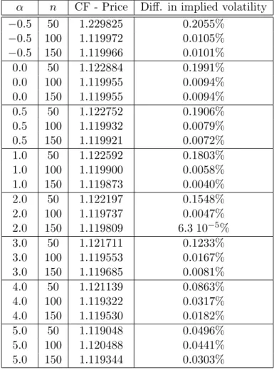
The quality examination covers20caps with varying lifetime, moneyness and implied volatility. Coming from an initial interest rate of7%the strikes change between6%(in-the-money),7%(at-the-money) and 8% (out-of-the-money). In the rst part we assume a implied volatility of20%and shift the starting time of the cap. We focus on caps starting in1,2,3,4and 5years and mature one year later. The results are summarized in Table 1 and are illustrated in Figure 1, Figure 2 and Figure 3. In addition we plotted the dierences in implied volatility in Figure 4.

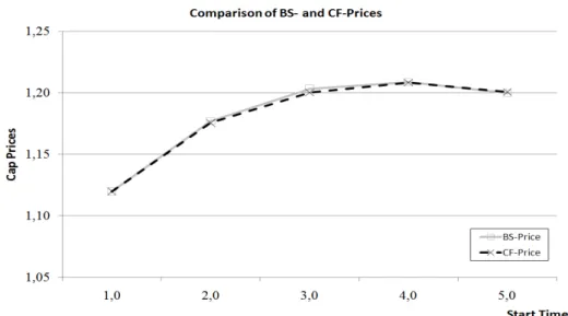
The results show that the prices computed by the characteristic function match the prices in the Black-Scholes model, which equal the prices com-puted by semi-closed formulas according to (Henrard 2003). The error in dierences in implied volatility is small and varies between the minimum of −0.1178% and the maximum of 0.1136%. The average of the signed dif-ferences is 0.0015% and the average of the absolute dierences amount to 0.0604%. Furthermore there is no noticeable trend in the error, like a sys-tematic over or under valuation. In 7 of 15 cases (47%) the characteristic

(40)

Implied V olatilit y Strik e Start Time Maturit y BS-Price CF-Price Price dierences Dierences in implied volatilit y 0.2 0.08 1.0 2.0 0.2357 0.2361 0.0004 0.0137% 0.2 0.08 2.0 3.0 0.3998 0.4031 0.0023 0.0702% 0.2 0.08 3.0 4.0 0.5071 0.5036 -0.0035 -0.0963% 0.2 0.08 4.0 5.0 0.5798 0.5818 0.0020 0.0500% 0.2 0.08 5.0 6.0 0.6290 0.6338 0.0048 0.1136% 0.2 0.07 1.0 2.0 0.5586 0.5558 -0.0028 -0.1178% 0.2 0.07 2.0 3.0 0.7083 0.7081 -0.0002 -0.0060% 0.2 0.07 3.0 4.0 0.7940 0.7974 0.0034 0.0936% 0.2 0.07 4.0 5.0 0.8449 0.8435 -0.0014 -0.0364% 0.2 0.07 5.0 6.0 0.8733 0.8773 0.0040 0.0996% 0.2 0.06 1.0 2.0 1.1198 1.1198 0.0000 -0.0001% 0.2 0.06 2.0 3.0 1.1769 1.1754 -0.0015 -0.0614% 0.2 0.06 3.0 4.0 1.2033 1.2002 -0.0031 -0.1060% 0.2 0.06 4.0 5.0 1.2087 1.2082 -0.0005 -0.0179% 0.2 0.06 5.0 6.0 1.1998 1.2006 0.0008 0.0234% 0.10 0.08 3.0 4.0 0.1542 0.1532 -0.0010 0.0317% 0.15 0.08 3.0 4.0 0.3250 0.3252 0.0002 0.0047% 0.20 0.08 3.0 4.0 0.5071 0.5036 -0.0035 -0.0963% 0.25 0.08 3.0 4.0 0.6929 0.6947 0.0017 0.0461% 0.30 0.08 3.0 4.0 0.8796 0.8834 0.0038 0.1015% Table 1: Presen tation of the results of pricing caps by characteristic functions (in the Ho-Lee Mo del) and in the Blac k-Sc holes Mo del. Further, w e state the errors in term s of dierences in implied volatilit y. The parameters lik e the strik e, the starting time an d the (original) implied volatilit y change.

(41)

Figure 1: Comparison of the Black-Scholes (BS) prices and the prices com-puted by characteristic functions (CF). The strike is xed at 8% (out-of-the-money), the starting time varies between 1 and 5 years and each caps matures one year.

Figure 2: Comparison of the Black-Scholes (BS) prices and the prices com-puted by characteristic functions (CF). The strike is xed at 7% (at-the-money), the starting time varies between1and5years and each caps matures one year.

(42)

Figure 3: Comparison of the Black-Scholes (BS) prices and the prices com-puted by characteristic functions (CF). The strike is xed at6% (in-of-the-money), the starting time varies between1and5years and each caps matures one year.

Figure 4: Presentation of the dierences in implied volatility between the Black-Scholes and characteristic function prices for caps. The solid line rep-resents caps with strike8%, the dashed one displays caps with strike7%and the dotted one brings out the dierences in implied volatility for caps with strike 6%. The errors corresponds to the cap prices in Figure 1, Figure 2 and Figure 3.

(43)

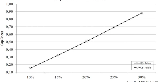
function delivers slightly higher values. These dierences result from nu-merical imprecisions generated by the multiplication of really high with low values. As described in Section 8 the accuracy of the pricing method in-creases by increasing the accuracy of the quadrature. Next to the change of strikes we analyzed the behavior of varying implied volatilities. Based on a strike of 8% we used implied volatilities of 10%, 15%, 20%, 25% and 30%. This test incorporates caps starting in 3 years and last 1 year. The results are presented in Table 1, Figure 5 and Figure 6. The error uctu-ates between −0.0963% and 0.1015% of implied volatility. The average of the signed dierences add up to 0.0048% and the average of the unsigned dierences is0.0561%. Again, one cannot state any trend in the errors as3 of5 (60%) prices computed by characteristic functions are higher.

Summarizing, we can observe that the pricing by characteristic functions is conform with the pricing by semi-closed formulas in the one-factor model. We tested the method by varying market situations and did not notice any noticeable systematic problems. Hence the numerical results validate the theoretical analysis.

Figure 5: Comparison of the Black-Scholes (BS) prices and the prices com-puted by characteristic functions (CF). The given implied volatility varies between0.1and0.3. The strike is xed at8%(out-of-the-money), the start-ing time varies between 1and 5years and each caps matures one year.

(44)

Figure 6: Presentation of the dierences in implied volatility between the Black-Scholes and characteristic function prices for caps. The errors corre-sponds to the cap prices in Figure 5.

8 Numerical Analysis

The pricing of interest rate derivatives by characteristic functions reduces to two main steps. First, the calculation of the model-dependant characteristic function by building up and solving a system of ODEs. Second, the com-putation of the pricing formulas including an inversion of the characteristic function according to Proposition 7.1. The computation of the character-istic function can be done analytically under some technical conditions as mentioned in Section 7. In contrast, the transform inversion has to be done numerically and the main problem reduces to the computation of an innite integral of the form

∞ Z 0 ImhΨχ(a+ıvb, X0,0, T) exp(−ıvy) i v dv. (19)

First, we investigate the behavior of the integrand close tov= 0and second, we focus on the eect of the numerical integration method.

(45)

8.1 Analysis of the Transform Inversion

The integrand has a singularity of order one inv = 0, but in the following we will show, that it is removable as the limitsv→0 exists.

Theorem 8.1.

We x the parameters a ∈ _Rn_, _b _∈

Rn, X0 = 0 ∈ Rn, T ∈ R. If the

characteristic of the general Cheyette Model χ = (H, K, ρ) is dened as in Section 5.2, then the limit

L= lim

v→0

Im[Ψχ₍_a₊_{ıvb, X}

0,0, T) exp(−ıvy)] v

exists and is given by

L= expRe[A(0, T, a)]h d

dvIm[A(0, T, a)]−y

i

.

Proof.

The characteristic function is dened by

Ψχ(u, X0,0, T) = exp[A(0, T, u) +B(0, T, u)X0]

as presented in Section 6.2. Using the initial conditionX0= 0, we obtain

Ψχ(u, X0,0, T) = exp(A(0, T, u)). ⇒ImhΨχ(a+ıvb, X0,0, T) exp(−ıvy) i = Im h exp(A(0, T, a+ıvb)−ıvy) i .

The complex-valued exponential function can be decomposed into real- and imaginary part as exemplarily presented forw∈_C

exp(w) = exp[Re(w)] [cos(Im(w)) +ısin(Im(w))] ⇒Im exp(w) = exp(Re(w)) sin(Im(w))

(46)

⇒Im[Ψχ(a+ıvb, X0,0, T) exp(−ıvy)]

= exphRe(A(0, T, a+ıvb)−ıvy)isinhIm(A(0, T, a+ıvb)−ıvy)i Thus, the integrandI(v)has the structure

I(v) =1 vexp Re[A(0, T, a+ıvb)−ıvy] sin Im[A(0, T, a+ıvb)−ıvy] .

In the following we want to apply the rule of L'Hôpital as presented in Appendix A.2. Therefore we have to verify that

(1) lim

v→0 exp(Re[A(0, T, a+ıvb)−ıvy]) sin(Im[A(0, T, a+ıvb)−ıvy]) = 0,

(2) lim

v→0 v= 0.

The second assumption is trivial and we have to investigate the rst one. If we could show, that both conditions are fullled, then the limit can be written as lim v→0I(v) = limv→0 1 vexp Re[A(0, T, a+ıvb)−ıvy] sin Im[A(0, T, a+ıvb)−ıvy] L'Hôpital = lim v→0 1 d dvv d dv exp Re[A(0, T, a+ıvb)−ıvy] sin Im[A(0, T, a+ıvb)−ıvy] = lim v→0 d dv exp Re[A(0, T, a+ıvb)−ıvy] sin Im[A(0, T, a+ıvb)−ıvy] . (20)

The singularity in v = 0 would be removed and we could focus on the last equation. But rst, we have to verify that

(47)

lim

v→0{exp(Re[A(0, T, a+ıvb)−ıvy])

sin(Im[A(0, T, a+ıvb)−ıvy])}= 0.

Therefore we will show lim

v→0Im[A(0, T, a+ıvb)−ıvy] = 0, (21)

lim

v→0exp(Re[A(0, T, a+ıvb)−ıvy]) =c <∞, (22)

which imply the desired proposition.

First, we concentrate on (21). The function A(t, T, u) is dened by a system of ordinary dierential equations (7) and (8). First, we have to solve the ODE (8) for B(t, T, u). In the general Cheyette Model with arbitrary number of factors, the ODE is given by

˙

B(t) =ρ1−K1T(t)B(t) (23)

B(T) =u (24)

with xed parametersρ1 ∈Rn,u∈Cn,K1 ∈Rn×n. As presented in Section 5.2, the matrixK1 ∈Rn×nis a diagonal matrix. Thus, the system of ODEs (23) is decoupled and can be solved in every dimensionj= 1, ..., nseparately,

˙

Bj(t) = (ρ1)j −(K1(t))jj(B(t))j

˙

Bj(T) =uj =aj +ıvbj.

This inhomogeneous ordinary dierential equation has a unique solution as exemplarily presented in (Walter 2000)

Bj(t) = exp − t Z T [K1(s)]jjds (a+ıvb)j+ t Z T  ρ1,jexp   l Z T [K1(s)]jjds    dl

The coecient matrixK1(t)andρ1 are real valued thus, the imaginary part

(48)

Im(Bj(t)) = exp − t Z T [K1(s)]jjds vbj. (25) with lim v→0Im[Bj(t)] = 0.

The functionA(t, T, u) is given as a solution to ˙ A(t) =ρ0−K0B(t)− 1 2B(t) T_H 0B(t), A(T) = 0,

with predened quantities ρ0 ∈R, B(t) ∈Cn,K0 ∈Rn and H0 ∈Rn. The unique solution is given directly via integration

A(t) = t Z T ρ0−K0(s)B(s)− 1 2B(s) T_H 0(s)B(s)ds = t Z T ρ0− n X j=1 (K0)jBj(s)− 1 2B(s) T   n X j=1 (H0)kjBj(s)  ds = t Z T ρ0− n X j=1 (K0)jBj(s)− 1 2 n X k=1 Bk(s)   n X j=1 (H0)kjBj(s)   k ds.

The complex valued integral can be decomposed in real- and imaginary part. The imaginary part is given by

Im(A(t)) = t Z T Im ρ0−K0(s)B(s)− 1 2B(s) T_H 0(s)B(s) ds

and can be divided into three summands: (1) Im(ρ0) = 0, asρ0 ∈R. (2) Im[K0(s)B(s)] = n X j=1 [K0]jIm[(B(s))j]

(49)

= n X j=1 (K0)jexp(− t Z T [K1(s)]jjds)vbj v→0 → 0 (3) Im[B(s)TH0(s)B(s)] = Im n X k=1 Bk(s) h_Xn j=1 (H0)kjBj(s) i k = Im n Re n X k=1 Bk(s) +ıIm n X k=1 Bk(s) o   n X j=1 (H0)kj[Re(Bj(s)) +ıIm(Bj(s))]   = Imh n X k=1 Bk(s) i | {z } →0, forv→0   n X j=1 (H0)kj[Re(Bj(s)) +ıIm(Bj(s))]   + Reh n X k=1 Bk(s) iXn j=1 (H0)kj Im[Bj(s)] | {z } →0, forv→0 v→0 → 0 This implies lim v→0Im(A(t, T,0)) = 0. ⇒ lim v→0Im(A(t, T,0)−ıvy) = lim v→0Im(A(t, T,0))−vy = 0

(50)

(22): lim

v→0exp [Re(A(0, T, a+ıvb)−ıvy)] = limv→0exp [Re(A(0, T, a+ıvb))]

The function exp [Re(A(0, T, a+ıvb))] is continuous with respect to v and

thus

lim

v→0exp [Re(A(0, T, a+ıvb))] = exp [Re(A(0, T, a))].

This function is bounded, if Re[A(0, T, a)] is bounded. Thus the condition (22) reduces to

Re[A(0, T, a)] = ˜c <∞.

According to previous calculations

A(t, T, a) = t Z T ρ0− n X j=1 (K0)jBj(s)− 1 2 n X k=1 Bk(s)   n X j=1 (H0)kjBj(s)   k ds ⇒Re[A(t, T, a)] = t Z T Re[ρ0]−Re   n X j=1 (K0)jBj(s)   −1 2Re   n X k=1 Bk(s)   n X j=1 [H0]kjBj(s)   k  ds

The coecientsρ0,K0,H0 are xed and nite. Thus, we have to investigate

the real part of Bj(s). If it is bounded, it follows that Re[A(0, T, a)] is

bounded and thus condition (22) is fullled,

Bj(t) = exp − t Z T (K1(s))jjds  a_j+ t Z T {(ρ1)jexp( l Z T (K1(s))jjds)}dl  .

(51)

andρ1 are xed and nite. Consequently,

Re[Bj(t)] =Bj(t) = ˜c <∞.

Thus, condition (22) is fullled. So far, we have proved Proposition (21) and (22), which were necessary conditions to apply the rule of l'Hôpital. According to (20), lim v→0I(v) = limv→0 d dv

expRe(A(0, T, a+ıvb)−ıvy)

sinhIm(A(0, T, a+ıvb)−ıvy)i = lim v→0 d dv exp Re(A(0, T, a+ıvb)) sin h Im(A(0, T, a+ıvb))−vy i = lim v→0 d dv h

exp(Re(A(0, T, a+ıvb)))isinhIm(A(0, T, a+ıvb))−vy

| {z }

→0forv→0

i

+ exphRe(A(0, T, a+ıvb))icoshIm(A(0, T, a+ıvb))−vy

| {z } →0forv→0 i n d dv Im(A(0, T, a+ıvb))−v o = lim v→0 exp Re(A(0, T, a+ıvb)) | {z } =˜c<∞_{according to (22)} d dvIm(A(0, T, a+ıvb))−y .

Finally, we have to show that lim

v→0

d

dvIm(A(0, T, a+ıvb)) is bounded. As

already shown, the imaginary part ofA(0, T, a+ıvb) can be written as

Im[A(0, T, a+ıvb)] = 0 Z T Im(ρ0)−Im K0(s)B(s) − 1 2Im B(s)TH0(s)B(s) ds.

(52)

derivation with respect tov just inuencesB(s). If we can show, that

lim

v→0 d

dv Im[B(s, T, a+ıvb)] =c1<∞,

holds, that would imply

d

dv Im[A(0, T, a+ıvb)] =c2 <∞.

The boundedness of this expression completes the proof. As shown in (25) Im Bj(s) = exp − s Z T (K1(l))jjdl vbj. ⇒ d dvIm Bj(s) = exp− s Z T [K1(l)]jjdl bj

The coecientsK1 andbj are xed and nite, thus _dvd_jImBj(s)is bounded,

which completes the proof concerning the existence of the limit. The limit is given by

L = lim v→0I(v) = lim v→0exp Re(A(0, T, a+ıvb)) h d dvIm(A(0, T, a+ıvb))−y i = expRe(A(0, T, a))h d dv Im(A(0, T, a))−y i

(53)

Theorem 8.2.

We x the parameters a ∈ _Rn_, _b _∈

Rn, X0 = 0 ∈ Rn, T ∈ R. The

characteristic χ = (H, K, ρ) representing the Ho-Lee Model is dened as in Section 5.2, then the limit

L= lim

v→0

Im[Ψχ(a+ıvb, X0,0, T) exp(−ıvy)] v

exists and is given by

L= exp h −f T + c 2_T 6 (−2T 2_{+ 3(}_{T a}₊_a2₎₎i c2_T 6 (3T b+ 2ab)−y . Proof.

In the Ho-Lee Model, the functionA(0, T, a+ıvb)is dened by

A(0, T, a+ıvb) =−f T +c 2_T 2 h −2T2+ 3T(a+ıvb) + 3(a+ıvb)2 i

Thus, the real and imaginary parts are given by

Re(A(0, T, a+ıvb)) = −f T +c2₆T[−2T2+ 3(T a+a2−v2b2)] and Im(A(0, T, a+ıvb)) = c2₆T[3T vb+ 2avb] ⇒ d dv{ImA(0, T, a+ıvb)} =c 2_T 6 [3T b+ 2ab]. This implies L= lim v→0exp Re(A(0, T, a+ıvb)) h d dv Im(A(0, T, a+ıvb)−y) i = exp h −f T +c 2_T 6 (−2T 2_{+ 3(}_{T a}₊_a2₎₎ihc2T 6 (3T b+ 2ab)−y i .

(54)

In addition to the analytical proof of the existence of the limit, we tested the behavior of the integrand close to zero numerically. The shape of the

integrand is determined by the model, the parameters a ∈ _Rn_, _b _∈

Rn,

y∈Rn, X0 ∈ Rn and T ∈ R+. We tested numerous parameter sets and

dierent (one-factor) models (n = 1) to understand the behavior close to zero. Mainly we identied two types of function shapes just depending on the parameter y ∈ R. If y is positive, the function is negative and strictly

increasing to 0 and if y is negative, the function has positive values and

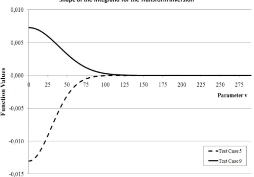
is strictly decreasing to 0. Exemplarily we plotted two integrand functions (Test case5 and 9) in the intervalv ∈[10−10,300] with step size h= 10−6 and the functions are shown in Figure 7.

Figure 7: Shape of the integrand of the transform inversion for two dierent parameter sets in the interval[10−10,300]and step sizeh= 10−6. Test Case 5: a=−6,b = 1,y = 0.018707283, x= 0, T = 5,c= 0.02, f = 0.06; Test Case9: a=−4,b= 1,y=−008943557,x= 0,T = 3,c= 0.02,f = 0.06.

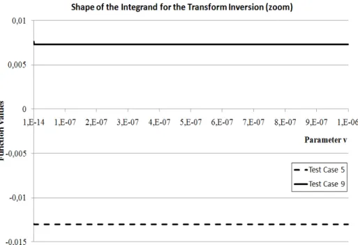
Furthermore, we concentrated on the function behavior in a small neigh-borhood of zero. Therefore, we evaluated the integrand in the interval [10−14,10−6]with a step size ofh= 10−12and plotted the results in Figure 8.