https://doi.org/10.1007/s11222-018-9842-2
A constrained regression model for an ordinal response with ordinal
predictors
Javier Espinosa1,2 ·Christian Hennig3,4
Received: 23 April 2018 / Accepted: 13 November 2018 © The Author(s) 2018
Abstract
A regression model is proposed for the analysis of an ordinal response variable depending on a set of multiple covariates containing ordinal and potentially other variables. The proportional odds model (McCullagh in J R Stat Soc Ser B (Methodol) 109–142,1980) is used for the ordinal response, and constrained maximum likelihood estimation is used to account for the ordinality of covariates. Ordinal predictors are coded by dummy variables. The parameters associated with the categories of the ordinal predictor(s) are constrained, enforcing them to be monotonic (isotonic or antitonic). A decision rule is introduced for classifying the ordinal predictors’ monotonicity directions, also providing information whether observations are compatible with both or no monotonicity direction. In addition, a monotonicity test for the parameters of any ordinal predictor is proposed. The monotonicity constrained model is proposed together with five estimation methods and compared to the unconstrained one based on simulations. The model is applied to real data explaining a 10-points Likert scale quality of life self-assessment variable by ordinal and other predictors.
Keywords Monotonic regression·Monotonicity direction·Monotonicity test·Constrained maximum likelihood estimation Mathematics Subject Classification62H12·62J05·62-07
1 Introduction
In many situations where regression models are suitable, the relationship between ordinal responses and ordinal predictors is of interest. However, statistical modelling for this type of relationship has called little attention. Even the literature for Electronic supplementary material The online version of this article (https://doi.org/10.1007/s11222-018-9842-2) contains supplementary material, which is available to authorized users.
B
Javier Espinosa[email protected]; [email protected] Christian Hennig
[email protected]; [email protected]
1 Department of Economics, USACH - Universidad de
Santiago de Chile, Santiago, Chile
2 Present Address: Department of Statistical Sciences,
University College London, London, UK
3 Dipartimento di Scienze Statistiche “Paolo Fortunati”,
Universita di Bologna, Bologna, Italy
4 Department of Statistical Sciences, University College
London, London, UK
ordinal predictors with any other type of scale of the response variable is scarce (see, for example, Tutz and Gertheiss2014 and Rufibach2010).
In order to account for an ordinal response variable, pro-portional odds cumulative logit models (McCullagh 1980) are used here in the presence of multiple predictors allowing for different measurement scales. We pay special attention to the treatment of ordinal scale predictors. Their parameter estimates are restricted to be monotonic through constrained maximum likelihood estimation (CMLE). To begin with, consider for simplicity one ordinal response variableywith kcategories and one ordinal predictorx with pcategories. The corresponding model for this setup is
logit[P(yi ≤ j|xi)] =αj + p
h=2
βhxi,h, (1)
j=1, . . . ,k−1.αjandβhforh=2, . . .pare real parame-ters. The observations are(xi,yi),i =1, . . . ,n. The vector
xi contains thexi,h, which are dummy variables defined as
xi,h=1 ifxifalls in theh-th category of the ordinal predic-tor and 0 otherwise, withh = 2, . . . ,p. Category number
1 is treated as the baseline category withβ1=0; therefore,
the dummy variablexi,1 = 1−
p
h=2xi,h is omitted and
the sum in model (1) starts ath =2. Monotonicity on{βh} is obtained by using CMLE. The general model is defined in Sect.2, which allows for multiple ordinal predictors and other covariates of different measurement scales.
The monotonic effects approach to the ordinal predictors treatment is conceived here as an intermediate point between two general and common approaches within the context of regression analysis on observed variables. One of these com-mon approaches corresponds to an unconstrained version of (1), treating the ordinal predictor as if it were nominal. This ignores the ordinal information. The other common approach treats an ordinal predictor as if it were of interval scale, replacing it by a single transformed variable after applying some scoring method, f. More formally,
logit[P(yi ≤ j|xi)] =αj+βx˜i, (2) withx˜= f(x). This treats f(x)as interval scaled. Numerous data-based methods for scaling of ordinal variables have been proposed in the literature, on top of using plain equidistant Likert scaling (see, e.g., Bross1958; Harter 1961; Tukey 1962; Hensler and Stipak1979; Brockett1981; Casacci and Pareto2015), but ultimately in most situations the data do not carry conclusive information about the appropriateness of any scaling f.
The intermediate approach proposed here is defined to achieve a set of linear estimates described by multiple mag-nitudes, as in the nominal scale approach, but allowing one direction only, as in the interval scale approach. The lat-ter is attained by restricting the effects of model (1) to be monotonic in either direction. The monotonicity assump-tion should not necessarily be taken for granted in regression with ordinal predictor and response. But it has a special sta-tus, similarly to linearity between interval-scaled variables. According to Stevens (1946) the interval scale is defined by the equality in the meaning of differences between values regardless of the location of these differences on the mea-surement range. A linear relationship between interval-scaled variables means that the impact of a change in the predictor on the response is proportional to the meaning of the change of measurement at all locations of the measurement scale. For the ordinal measurement scale, only the order of measured values is meaningful. In this case, monotonic relationships are those that imply that a change in the predictor of the same meaning (i.e., changing to a value that is higher, or lower, respectively) at all locations of the measurement scale has an effect of the same meaning on the response.
Some other regression models for ordinal predictors are also based on the monotonic effects assumption. However, models for ordinal responses have not been explicitly dis-cussed in this context. Tutz and Gertheiss (2014) used
penalisation methods for modelling rating scales as predic-tors, and an active set algorithm was proposed by Rufibach (2010) to incorporate ordinal predictors in some regression models considering the response variable to be continuous, binary, or represent censored survival times, and assuming isotonic effects of the ordinal predictors’ categories. Another related method is isotonic regression, mostly applied to con-tinuous data (see, for example, Barlow and Brunk 1972; Dykstra and Robertson1982; Stout2015). In a broader con-text, there are some other types of statistical models that deal with ordinal data, such as those in item response theory (IRT) (e.g., Tutz1990; Bacci et al.2014), latent class models (e.g., Moustaki2000,2003; Vasdekis et al.2012), nonlinear prin-cipal components analysis (NLPCA) (e.g., De Leeuw and Mair2009; Linting and van der Kooij2012; Mori et al.2016), and nonlinear canonical correlation analysis (NLCCA) (e.g., Mardia et al. 1979; De Leeuw and Mair 2009). However, their settings are somewhat different compared to the one corresponding to modelling an ordinal response with ordinal predictors (and others) in classical regression. For instance, unlike IRT models and latent class models, classical regres-sion models do not assume latent variables; and in contrast to NLPCA and NLCCA, classical regression models are not used as a dimensionality reduction technique and need a sin-gle dependent variable, respectively.
The monotonicity constrained regression model discussed here can be used for several purposes. When the uncon-strained parameter estimates associated with the ordinal predictor are monotonic, then clearly there is no need of a constrained model. However, when these unconstrained esti-mates are non-monotonic, then there are some reasons why the constrained model could be useful. It is often of interest to compare unconstrained and constrained fits in order to decide whether there is evidence for non-monotonic relationship. In case that the unconstrained version does not provide a clearly better fit, the monotonic fit may be superior regarding inter-pretability, and may also lead to a smaller mean square error, as will be shown by simulations and a real data application. In Sect. 2, the proposed model is developed in detail to obtain both constrained parameter estimates for multi-ple ordinal predictors and unconstrained estimates for other types of covariates. As the monotonic estimates can be either increasing (isotonic) or decreasing (antitonic), it is neces-sary to specify this relation while defining the constraints. Also, investigating possible directions of monotonicity for all ordinal predictors is of interest in its own right. Therefore, a monotonicity direction classification (MDC) procedure is introduced in Sect.3that determines the best possible com-bination of isotonic and/or antitonic associations as a way of assisting the estimation method of the constrained model introduced in Sect.2. In Sect.4, a monotonicity test is pro-posed as a complementary tool to assess the validity of the monotonicity assumption of each ordinal predictor. Both the
MDC procedure and the monotonicity test provide statisti-cal evidence on the validity of the monotonicity assumption. This can be incorporated in the estimation procedure; Sect.5 presents four approaches, one based on the monotonicity test and three based on the MDC procedure. On the other hand, the same procedures may also detect that the data are con-sistent with zero influence of a variable, in which case the variable may be dropped, this is treated in Sect.5.3. Simu-lations are presented in Sect.6comparing the mean square error and standard error between the constrained and uncon-strained approaches. Finally, the proposed model is applied to real data from the Chilean National Socio-Economic Charac-terisation in Sect.7. A quality of life self-assessment variable using a 10-points Likert scale is analysed considering ordinal and other predictors.
2 Proportional odds with monotonicity
constraints
For an ordinal response variableywithkcategories, letyibe the response category for subjecti. The model of proportional odds is
logit[P(yi ≤ j|xi)] =αj+βxi, (3)
j =1, . . . ,k−1, i=1, . . . ,n.A part of the elements ofβ corresponds to those effects associated with ordinal predic-tors categories inx, for which their parameter estimates are constrained to account for monotonicity as explained later.
When this model has one or more of both ordinal and non-ordinal predictors, it can be represented as
logit[P(yi≤ j|xi)] =αj+ t s=1 ps hs=2 βs,hsxi,s,hs+ v u=1 βuxi,u, (4) wherexi is a vector withv−t+
t
s=1ps elements repre-senting a set oftordinal predictors (OP) and theirts=1ps categories together with v non-ordinal predictors for the i-th observation. Each ordinal predictor is denoted by the subindex s, with s = 1, . . . ,t, and contributes ps −1 dummy variables to the model representing its ordinal cat-egories{1, . . . ,ps}assuming the first one as the baseline category, thusβs,1 = 0. Note that differences between the
regression parameters belonging to the ordinal categories are independent of the baseline category. We later use con-fidence intervals (CIs) for these parameters, the widths of which can depend on the baseline category. For ordinal vari-ables, the beginning or end point of the scale seems natural choices. Each dummy variable is defined asxi,s,hs = 1 if thei-th observation falls in the category hs of the ordinal
predictorsand 0 otherwise, withhs =1, . . . ,ps. Therefore,
xi = (xi,1,2, . . . ,xi,1,p1,xi,2,2, . . . ,xi,2,p2, . . . ,xi,t,2, . . . ,
xi,t,pt,xi,1, . . . ,xi,v), where those variables with three indexes correspond to the observation of an ordinal predictor category and those with two are observations of other types of covariates.
2.1 Likelihood model fitting
Define πj(xi) = P(yi = j|xi), the probability of the response of subjectito fall in categoryj, and letyi1, . . . ,yi k be the binary indicators of the response for subjecti, where yi j = 1 if its response falls in category j and 0 otherwise. Therefore, for independent observations, the likelihood func-tion is based on the product of the multinomial mass funcfunc-tions for thensubjects:
L({αj},β) = n i=1 k j=1 πj(xi)yi j = n i=1 k j=1 P(yi = j|xi)yi j = n i=1 k j=1 [P(yi ≤ j|xi)−P(yi ≤ j−1|xi)]yi j = n i=1 ⎧ ⎨ ⎩ k j=1 eαj+ts=1 ps hs=2βs,hsxi,s,hs+vu=1βuxi,u 1+eαj+ts=1 ps hs=2βs,hsxi,s,hs+vu=1βuxi,u − eαj−1+ t s=1 ps hs=2βs,hsxi,s,hs+vu=1βuxi,u 1+eαj−1+ts=1 ps hs=2βs,hsxi,s,hs+vu=1βuxi,u yi j ⎫⎬ ⎭. (5) Hence, πj(xi)= eαj+ts=1 ps hs=2βs,hsxi,s,hs+vu=1βuxi,u 1+eαj+ts=1 ps hs=2βs,hsxi,s,hs+vu=1βuxi,u − eαj−1+ t s=1 ps hs=2βs,hsxi,s,hs+ v u=1βuxi,u 1+eαj−1+ts=1 ps hs=2βs,hsxi,s,hs+vu=1βuxi,u, (6) and the log-likelihood function for the model is
({αj},β)= n i=1 k j=1 yi jlogπj(xi). (7) As we are interested in a constrained version of this model with the aim of getting monotonic increasing/ decreasing effects, it is necessary to define the set of constraints to be
applied on thet sets of ps coefficients. The isotonic con-straints are
0≤βs,2≤ · · · ≤βs,ps, ∀s∈I, (8) whereI ⊆ S, withS = {1,2, . . . ,t}, andβs,1 = 0. The
antitonic constraints are
0≥βs,2≥ · · · ≥βs,ps, ∀s∈A, (9) whereA⊆ S, andβs,1 =0. An estimation method based
on a monotonicity direction classification (MDC) procedure will be discussed in Sect.3, allocating the ordinal predictors in either of these two subsets, achievingI∪A=S.
These constraints can be expressed in matrix form as
Cβ(or d) ≥ 0. The vector β(or d) is part of the vector β. The latter contains all the parameters associated with the tordinal predictors and theirps−1 categories together with thevnon-ordinal predictors,β=
β(or d),β(nonor d)
, with β
(or d) =(β1, . . . ,βt)withs =1, . . . ,t,andβ(nonor d) =
(β1, . . . , βv)withu = 1, . . . , v, where each vector βs =
(βs,2, . . . , βs,ps) withhs = 2, . . . ,ps. The matrix Cis a square block diagonal matrix ofts=1(ps−1)dimensions composed oftsquare submatricesCsin its diagonal structure and zeros in its off-diagonal blocks as follows:
C= ⎡ ⎢ ⎢ ⎢ ⎣ C1 0 · · · 0 0 C2 0 0 0 · · · ... 0 0 · · · ·Ct ⎤ ⎥ ⎥ ⎥ ⎦, withs=1, . . . ,t, where Cs = ⎡ ⎢ ⎢ ⎢ ⎣ 1 0 · · · 0 −1 1 0 0 0 ... ... 0 0 · · · −1 1 ⎤ ⎥ ⎥ ⎥ ⎦ ∀s∈I, Cs = ⎡ ⎢ ⎢ ⎢ ⎣ −1 0 · · · 0 1 −1 0 0 0 ... ... 0 0 · · · 1 −1 ⎤ ⎥ ⎥ ⎥ ⎦ ∀s∈A,
and each square submatrixCs hasps −1 dimensions. Then, the maximisation problem is
maximise({αj},β)
subject toCβ(or d)≥0, (10)
where0is a vector ofts=1(ps −1)elements. Now, (10) can be expressed as the Lagrangian
L({αj},β,λ)=({αj},β)−λCβ(or d), (11)
whereλis the vector ofts=1(ps−1)Lagrange multipliers denoted byλs,hs.
The set of equations to be solved is obtained by differ-entiating L({αj},β,λ)with respect to its parameters and equating the derivatives to zero. In order to solve this in R(R Core Team2018), the packagemaxLik(Henningsen and Toomet2011) offers themaxLikfunction which refers
toconstrOptim2. This function uses an adaptive barrier
algorithm to find the optimal solution of a function sub-ject to linear inequality constraints such as in (10) (Lange 2010).
3 Monotonicity direction classification
Under the monotonicity assumption for all OPs, an impor-tant decision to be made is whether each ordinal predictor’s set of effects (also referred to as pattern), is either isotonic, namelys ∈I, or antitonic,s∈A. Also outside the context of parameter estimation, it may be of interest whether a pre-dictor is connected to the response in an isotonic or antitonic way, or potentially whether monotonicity may not hold or whether both directions are compatible with the data.
One possible way to deal with this decision is to just maximise the likelihood, i.e., to fit 2t models, one for each possible combination of monotonicity directions for the t ordinal predictors, and then choose the one with the high-est likelihood. However, as the number of ordinal predictors t increases, the number of possible combinations of mono-tonicity directions becomes greater, which could lead to a considerable number of models to be fitted, each involving a large number of covariates.
Another possible estimation method uses a monotonic-ity direction classifier to find the monotonicmonotonic-ity direction for each ordinal predictor and then fits only one model. This will be based on CIs for the parameters and on checking which monotonicity direction is compatible with these. This may miss the best model, but in some situations it may be desir-able to take into account fewer than 2tbut more than a single model.
The two approaches are put together in a three steps mono-tonicity direction classification (MDC) procedure exploiting their best features. Each of the first two steps uses a deci-sion rule with different confidence levels for the CIs, and the last step applies the multiple models fitting process described above over those patterns with no single monotonicity direc-tion established in the previous steps. Before describing its steps, consider some remarks and definitions.
The parameters’ CIs from an unconstrained model are the main input for the decision rule proposed here. It is possible to compute the CI defined in Eq. (12) for the parameters of an unconstrained version of model (4) (Agresti2010). Denote S Eβˆas the standard error of the parameter estimateβˆ, then
an approximate confidence interval forβwith a 100(1− ˜α)% confidence level is
ˆ
β±zα/˜ 2(S Eβˆ), (12)
wherezα/˜ 2denotes the standard normal percentile with
prob-abilityα/˜ 2. The values forβˆandS Eβˆare obtained by fitting the proportional odds model (McCullagh 1980) over the unconstrained model (4). TheRfunctionvglmof the pack-ageVGAMwas used here (Yee2018).
The first two steps of the MDC procedure provide four pos-sible outcomes for each pattern of unconstrained parameter estimates associated with an ordinal predictor’s categories: ‘isotonic’, ‘antitonic’, ‘both’, and ‘none’. The first two corre-spond to a classification of monotonicity direction, whereas the remaining two to the case where a single direction is not found because either both directions of monotonicity are possible or the parameter estimates’ pattern is not compatible with monotonicity, respectively. The idea is that the intersec-tions of all CIs for the parameters of a single ordinal predictor together will either allow for isotonic but not antitonic param-eters, or for antitonic but not isotonic paramparam-eters, or for both, or for neither. Formally, the MDC of the parameter estimates’ pattern is defined as ds,˜c= ⎧ ⎨ ⎩ isotonic ifDs,˜c= {0,1}orDs,˜c= {1} antitonic ifDs,˜c= {−1,0}orDs,˜c= {−1} both ifDs,˜c= {0} none ifDs,˜c⊇ {−1,1}, (13) whereDs,˜c= {ds,hs,hs,˜c}is defined as the set of distinct val-ues resulting from (14) for the ordinal predictorsconsidering confidence intervals with a 100c˜% confidence level, and
ds,hs,hs,˜c= ⎧ ⎨ ⎩ 1 ifL˜s,hs,˜c≥ ˜Us,hs,˜c −1 ifU˜s,hs,˜c≤ ˜Ls,hs,˜c 0 otherwise, (14) ∀h
s < hs and hs ∈ {2,3, . . . ,ps}, where U˜s,hs,˜c is the confidence interval’s upper bound of the parameter βs,hs associated with the categoryhs of the ordinal predictor s given a 100c˜% confidence level, andL˜s,hs,˜cis its correspond-ing lower bound. Note that, by definition, the first category of all ordinal predictors is set to zero, soL˜s,1,˜c= ˜Us,1,˜c =0,
∀s. (14) yields 1 when the CI of the parameterβs,hs is fully above the one ofβs,hs, and consequently, their CIs only allow an isotonic pattern; -1 when it is fully below pointing to an antitonic pattern; and 0 when there exists an overlap, meaning that both monotonicity directions are still possible.
Each result of (14), denoted asds,hs,hs,˜c, can be under-stood as an indicator of the relative position of the confidence
interval of the parameterβs,hs compared to the one ofβs,hs,
∀hs < hs andhs ∈ {2,3, . . . ,ps}, belonging to the same ordinal predictorsand given a 100c˜% confidence level. As this is a pairwise comparison, there exist ps(ps−1)/2 indi-cators for each ordinal predictors. Equation (13) uses these indicators to classify the monotonicity direction of an ordinal predictor as a whole at a particularc˜.
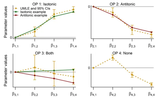
As an illustration, Fig.1 shows some arbitrary patterns representing a particular example for each one of the pos-sible results of (13). For instance, OP 1 is classified as ‘isotonic’ because all but one of the results of (14) are 1, where the only different is d1,4,3,0.95 = 0, and
there-foreD1,0.95 = {0,1}. The monotonicity direction of OP 2
is clear also, for which the results of (14) are −1 except for d2,4,3,0.95 = 0, with which (13) classifies this OP as
‘antitonic’. All the individual confidence intervals of OP 3 jointly overlap and contain zero. Therefore,d3,h3,h3,0.95=0
∀h
3<h3and thusD3,0.95= {0}, classifying OP 3 as ‘both’.
Finally, each individual confidence interval associated with the OP 4 is either fully above or fully below the ones of previous categories belonging to the same ordinal predic-tor. In particular,D4,0.95 = {−1,1}because, for example,
d4,2,1,0.95=1 andd4,3,2,0.95= −1, which (13) classifies as
‘none’.
The three steps MDC procedure has the following struc-ture:
Step 1 Setc˜at a relatively high 100c˜% confidence level, say 0.99, 0.95 or 0.90, and apply the MDC (13) to assign the subindexesseither to the setI orAdefined in Sect. 2.1. Therefore, I1 = {s : ds,˜c = isotonic} andA1 = {s : ds,˜c = antitonic}, where I1 and
A1 denote the isotonic and antitonic sets
result-ing from the step 1 respectively. In addition, define
B1= {s:ds,˜c=both}andN1= {s:ds,˜c=none}.
If(I1∪A1) = S, then all the ordinal predictors’
monotonicity directions have been decided, and there is no need to continue with the MDC procedure. Oth-erwise, the following step is used for the remaining cases only,(B1∪N1).
Step 2 Consider the set of ordinal predictors {s : s ∈ (B1∪N1)}and apply the MDC (13) in an iterative
manner while varying the confidence level 100c˜%. A decrease/increase ofc˜reduces/enlarges the range of the CIs of the parameterβs,hs ∀s ∈ (B1∪N1)
andhs ∈ {2,3, . . . ,ps}. These changes inc˜produce different effects on the classification depending on whethers ∈ B1ors ∈ N1, which must be used as
follows:
(a) For each s ∈ B1, the second step is to gradually
decreasec˜while applying the decision rule (13) using a new confidence level c˜ instead of c˜, obtaining
Fig. 1 Illustration of particular examples for each possible monotonicity direction classification
ds,˜cs. The level of c˜s must be gradually decreased until either a pre-specified minimum confidence level referred to as tolerance level c˜∗s is reached, with 0<c˜∗s <c˜, or the ordinal predictorsis classified as either isotonic or antitonic byds,˜cs.
(b) Conversely, for eachs ∈ N1, gradually increase c˜
while applying MDC (13) using a new confidence levelc˜sobtainingds,c˜s. The level ofc˜s must be grad-ually increased until either a pre-specified maximum confidence level referred to as tolerance levelc˜s∗is reached, withc˜<c˜∗s <1, or the ordinal predictors is classified as either isotonic or antitonic byds,˜cs.
Finally,I2 = I1∪ {s : ds,˜cs =isotonic ords,˜cs = isotonic}andA2 = A1∪ {s : ds,˜cs =antitonic or
ds,c˜s =antitonic}, where the subindex ofI2andA2
denotes results from the second step. After complet-ing the second step, if(I2∪A2)=S, then it is not
necessary to continue with step 3 and the MDC pro-cedure ends. If(I2∪A2) ⊂ S, then the third and
final step must be carried out.
Step 3 Fit 2#{s:s∈(I/ 2∪A2)} models accounting for possible
combinations of monotonicity directions of the ordi-nal predictors that were not classified as ‘isotonic’ or ‘antitonic’, i.e., those in the set{s:s∈/(I2∪A2)},
and choose the best model based on some optimality criterion, such as the maximum likelihood as used here.
In general, the MDC procedure describes two levels of decision. The first one is provided by step 1, where a con-fidence level is applied to all ordinal predictors by the use of a single parameterc˜. The second one is in step 2, where each ordinal predictors ∈(B1∪N1)is classified based on
its own confidence level. Step 2 allows to classify predictors
that were not classified based on the fixed initial confidence level.
In step 2, classifying more parameter estimates’ patterns withs∈B1as either isotonic or antitonic requires a gradual
reduction of the confidence level. The tolerance levelsc˜s∗and
˜
c∗s determine the leeway allowed for the confidence levels in order to enforce a decision. The choice of these may depend on the number of ordinal variables; if the number is small, running step 3 may not be seen as a big computational prob-lem, and it may not be necessary to enforce many decisions in step 2. The tolerance levelc˜∗s should not be too low, less than 0.8, say, because it is not desirable to make decisions based on a low probability of occurrence.
For thoses ∈ N1in step 2, the researcher does not face
such a trade-off, because greater confidence levels could increase (not decrease) the number of new isotonic or anti-tonic classifications for thoses∈N1.
It is important to reduce (or increase) the confidence level in step 2 in a gradual manner, by 0.01 or 0.005, say, for each iteration. If the chosen intervals in the sequence of confi-dence levels to be assessed are too thick without assessing intermediate levels, then, for an ordinal predictors ∈B1, it
is possible to switch its classification from ‘both’ to ‘none’ instead of updating it from ‘both’ to either ‘isotonic’ or ‘anti-tonic’. Conversely, the class of an ordinal predictors∈ N1
could change from ‘none’ to ‘both’. The thinner the inter-vals in the sequence of confidence levels to be assessed are, the less likely it is to switch from ‘both’ to ‘none’ or ‘none’ to ‘both’. However, in some specific cases, there still is a probability of having such an undesired class change.
The researcher may also be interested in exploring other monotonicity directions rather than those resulting from the MDC procedure proposed here, although the maximum like-lihood attained by the MDC procedure would not be reached.
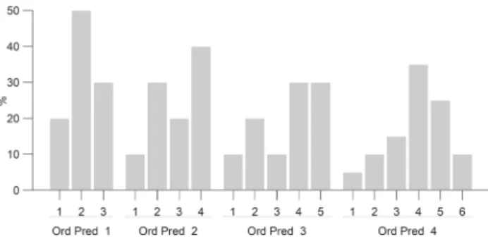
Fig. 2 Distributions of simulated ordinal predictors
In this case, the correspondence of each ordinal predictorsto eitherIorAshould simply be enforced when constructing
C, the matrix of constraints, as described in Sect.2.1. In order to illustrate the MDC procedure, we consider a particular example of model (4) with four ordinal predictors only (t = 4 andv =0), where p1 = 3, p2 = 4, p3 = 5,
p4 = 6, and k = 4, i.e., j = 1,2,3. The parameters are
chosen to beα1= −1,α2= −0.5, andα3= −0.1; and
β1=(1.0,1.5),
β2=(0.1,0.2,0.25),
β3=(−0.02,−0.04,−0.041,−0.05), and
β4=(−0.2,−0.3,−0.31,−0.35,−0.36).
These parameters represent a situation in which all covariates are monotonic, with the elements ofβ1andβ2being isotonic, and those ofβ3andβ4antitonic patterns. Given
monotonic-ity, the higher the distances between adjacent parameters are, the clearer the monotonicity direction is. In this illustration, these distances were chosen to make the monotonicity direc-tion clear for the first ordinal predictor only and less clear for the remaining ones,s=3 being the most unclear and chal-lenging case because all of its parameters show little distance between adjacent categories and consequently from zero.
The 2000 simulated observations of the ordinal predictors were obtained from the population distributions shown in Fig.2.
Using this simulated data set, an unconstrained version of the model was fitted to obtain the parameter estimates and their standard errors, with which a confidence interval can be computed for any level ofα˜ using Eq. (12).
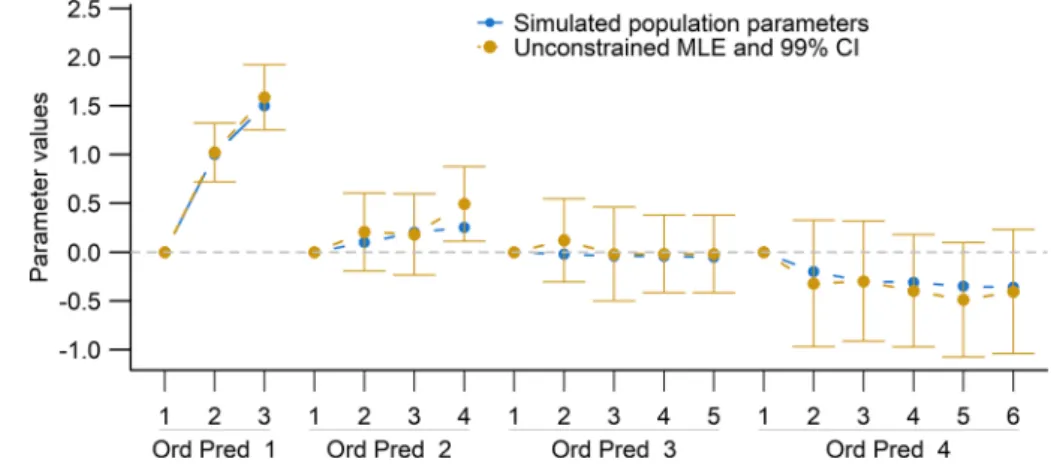
For the first step of the MDC procedure, the confidence level was set at a highc˜ = 0.99. The resulting confidence intervals allowed to classify the first and second OP as ‘isotonic’,I1 = {1,2}, and the remaining two patterns of
parameter estimates as ‘both’,B1= {3,4}. Figure3shows
that the latter two ordinal predictors allowed both directions of monotonicity, which is the reason why they were not clas-sified as ‘antitonic’. The second step was applied over each ordinal predictors ∈B1 = {3,4}using the same tolerance
level, c˜3∗ = ˜c∗4 = 0.8. Fors = 3, it was not possible to classify its pattern as ‘antitonic’ before reaching the toler-ance level. Therefore, it remained as ‘both’. Fors =4, the procedure was applied until reachingc˜s =0.96, where the fourth OP was classified as ‘antitonic’. Now,I2= {1,2}and
A2 = {4}. As no monotonicity direction was identified for
the third OP, two models were fitted in step 3 of the MDC procedure, one treating the third OP as ‘isotonic’ and the other one as ‘antitonic’. Finally, the model with the highest log-likelihood was selected as the final one.
The procedure successfully classified the ordinal pre-dictors s = 1,2,3,4 as ‘isotonic’, ‘isotonic’, ‘antitonic’, and ‘antitonic’, respectively, despite the fact that the uncon-strained parameter estimates of the last three are not mono-tonic. Furthermore, it reduced the number of possible models to be fitted from 17 (the unconstrained model and 16 con-strained models) to 3 (the unconcon-strained and two models in step 3) while making decisions based on individual confi-dence levels of 96% or greater.
As shown in Fig. 3, it is not easy to classify cases like s=3 where all the parameter estimates are close to zero and their confidence intervals are big enough to make the mono-tonicity direction classification infeasible for any reasonable tolerance level. In this case, the tolerance level would have needed to be set atc˜3∗≤0.53 had we wanted the MDC proce-dure to classify the third ordinal predictor as either ‘isotonic’ or ‘antitonic’. In fact, when doing so, the MDC makes a mis-take and classifies it as ‘isotonic’. This relationship between low tolerance levels and misclassification is the main reason why the procedure needs to start with a relatively high con-fidence levelc˜s and then gradually decrease it until reaching a reasonable tolerance level if necessary.
In cases likes =3, one option is to remove this variable from the model because all of the CIs associated with it con-tain zero even if we choose a tolerance level lower than 0.80, which we consider too low. Removing this variable would have allowed us to fit just two models (the unconstrained and one constrained) instead of three in the whole procedure. However, removing variables may not be good if the aim is to obtain a model with optimal predictive power.
4 A monotonicity test
The MDC procedure assists the decision on the choice of an appropriate monotonicity direction assumption for each OP when fitting model (4), but it is not a formal monotonicity test. It relies on the analysis of multiple pairwise comparisons of confidence intervals with flexibly chosen confidence levels without caring about the simultaneous error probability.
When analysing the monotonicity assumption on the parameters associated with an OPs, the Bonferroni correc-tion method can be used to construct a formal monotonicity
Fig. 3 Parameters of ordinal predictors’ categories and their unconstrained estimates with 99% confidence intervals
test for an OP. The Bonferroni correction method allows to compute a set of confidence intervals achieving at least a 100(1−αs∗)% confidence level simultaneously (see Miller
1981, p. 67, and Bonferroni 1936), which is the probabil-ity that all the parameters are captured by the confidence intervals simultaneously. For a given ordinal predictorsand a pre-specified αs∗, if each one of the ps −1 confidence intervals is built with a 100(1−αs∗/(ps −1))% confidence level, then the simultaneous confidence level will be at least 100(1−αs∗)%.
The null hypothesis ‘H0 :The parameters{βs,hs :hs = 1,2, . . . ,ps}are either isotonic or antitonic’ (0 ≤ βs,2 ≤
βs,3· · · ≤βs,ps (isotonic) and 0 ≥βs,2 ≥ βs,3· · · ≥βs,ps (antitonic)) is tested against the alternative ‘H1:The
param-eters{βs,hs : hs = 1,2, . . . ,ps}are neither fully isotonic nor fully antitonic’ for a given OPs, and settingβs,1=0 as
in previous sections.
For a given ordinal predictors, and taking advantage of the ordinal information provided by its categories, it is then checked whether all the confidence intervals simultaneously are compatible with monotonicity.
In order to identify whether there are pairs of confidence intervals ofβs,hs that are incompatible with monotonicity, a slight modification of Eqs. (13) and (14) is used. Now, instead of the confidence levelc˜, those equations useb˜ = 1−α∗s/(ps −1). Therefore, the monotonicity test for an ordinal predictorsis
Ts,b˜=
reject H0 ifDs,b˜⊇ {−1,1}
not reject H0 otherwise
(15)
where Ds,b˜ = {ds,hs,hs,b˜}is defined as the set of distinct values resulting from using Eq. (14) for the ordinal predic-tor s considering each confidence interval with a 100b˜% confidence level (instead of 100c˜%) in order to achieve a simultaneous confidence level of at least 100(1−α∗s)% for the parameters associated with the OPs.
IfTs,b˜ =reject H0, then the parameters associated with
the ordinal predictors are not compatible with the
mono-tonicity assumption with a simultaneous confidence level of at least 100(1−αs∗)%.
When applying this monotonicity test to the four OPs of the illustration discussed in Sect.3and using a pre-specified
α∗s =0.05, all the OPs were found to be compatible with the monotonicity assumption.
For a given pre-determined significance level ofα∗s (say 0.1, 0.05 or 0.01), the Bonferroni correction will often be very conservative, and it will be the more conservative the higher the number of ordinal categories involved in the monotonicity test is. A higher ps implies larger ranges of the intervals, making the test more likely to not rejectH0.
In order to show some results for the monotonicity test with OPs for which their association with the response vari-able is truly non-monotonic, consider a setting for model (4) with two OPs only (t =2 andv =0), where p1 =4,
p2 = 5, andk = 4, i.e., j = 1,2,3. The parameters for
the intercepts areα1 = −1,α2 = −0.5, andα3 = −0.1;
and the true sets of parameters of the OPs 1 and 2 represent non-monotonic associations, beingβ1=(0.4,1.7,0.8)and β
2=(−0.25,−0.7,−0.05,0.40). The distributions among
categories of OPs 1 and 2 are the same as the ones shown in Fig.2for OPs 2 and 3 correspondingly, and the number of observations is 2000.
After fitting the new unconstrained model on 1000 sim-ulated data sets and testing for monotonicity, the null
Fig. 4 True parameter patterns simulating non-monotonicity with dif-ferent rejection rates of the monotonicity test
hypothesis was rejected in 84.9% of the data sets for the OP 1 and in 84.5% for the second OP, in both cases withαs∗=0.05. Figure 4 shows the patterns of these non-monotonic OPs together with additional patterns with which rejection rates of around 5% are obtained (4.5% and 5.5% respectively).
5 Dropping constraints and variable
selection
5.1 Dropping monotonicity constraints using the
monotonicity test
The MDC procedure described in Sect.3 implies that the parameter estimates of all OPs are restricted to be monotonic. However, the researcher may want to drop monotonicity con-straints on OPs in case that there is clear evidence against monotonicity.
The monotonicity test proposed in Sect.4 can be used as a complementary tool to the MDC procedure in order to assist the estimation process. If the researcher is open to the possibility of not imposing the monotonicity constraints on some OPs, then he/she could first test monotonicity on each one of them, then drop the monotonicity constraints on those OPs for which the null hypothesis was rejected, and finally perform the MDC procedure imposing monotonicity constraints on all the remaining OPs. Under this scenario, in case that monotonicity is rejected for an OP, it would be more prudent to fit unconstrained estimates on the parameters associated with it. Therefore, such an OP should not be part
ofS, the set of OPs to be constrained, but rather part of the
non-ordinal predictors, considering it at the nominal scale level.
5.2 Dropping monotonicity constraints using the
MDC procedure
When dropping the monotonicity constraint for some of the OPs is considered as a feasible option, then not only the approach introduced in Sect. 5.1 could be used, but also three alternative ones that are proposed in this section. As in the previous section, consider the case where the researcher might also want to explore whether the monotonicity assump-tion holds for all of the OPs or for a subset of them, but now using a less conservative (i.e., dropping constraints more eas-ily) approach than the one based on the monotonicity test. We propose three additional methods. Two of them are based on the first and second steps of the MDC procedure correspond-ingly (‘CMLE MDC S1’ and ‘CMLE MDC S2’), and another one is based on a slight modification of the MDC procedure (‘CMLE filtered’).
5.2.1 CMLE MDC S1
Both monotonicity constraints and monotonicity directions are established using the first step of the MDC procedure. Once it determinesI1andA1, the monotonicity constraints
are dropped for the remaining ordinal predictors {s : s ∈/ (I1∪A1)}, namely{s:s∈(B1∪N1)}. Therefore, there is
no need of executing further steps.
The model is fitted imposing monotonicity constraints on ordinal predictors{s:s∈(I1∪A1)}using their
correspond-ing monotonicity directions, which requires to consider the ordinal predictors {s : s ∈ (B1∪N1)}as nominal scaled
variables.
This method is the least conservative one because it assumes that if a monotonic pattern is not established without adjustment of the confidence level 100c˜%, then the mono-tonicity constraint has to be dropped.
5.2.2 CMLE MDC S2
This method follows the same structure as the previous one but executing the MDC procedure until the end of its second step. Therefore, the third step is not executed and the model is fitted imposing monotonicity constraints on ordinal pre-dictors{s :s ∈(I2∪A2)}only, using their corresponding
monotonicity directions according toI2andA2, and
assum-ing the ordinal predictors{s : s ∈/ (I2∪A2)}as nominal
scaled variables.
5.2.3 CMLE filtered
An adjusted version of the MDC procedure described in Sect.3allows to drop the monotonicity assumption for some OPs. There are only two adjustments, one in step 2.b and the other one in step 3. The first one is to setc˜∗s = ˜c, i.e., the tolerance level for each OPs ∈N1is set to be the same as
the confidence level chosen in step 1. Therefore, the second step is not performed on any ordinal predictors∈ N1. The
second modification is to apply step 3 over the possible com-binations of monotonicity directions of the ordinal predictors that were classified as ‘both’ by the end of step 2, i.e., the number of models to be fitted is now 2#{s:ds,c˜s=both}instead of 2#{s:s∈(I/ 2∪A2)}. This implies thatS, the set of OPs to be
constrained, must be updated excluding each ordinal predic-tors∈N1from the set of monotonicity constraints. Finally,
the model should be fitted considering these OPs as nominal scaled variables.
These adjustments are equivalent to considering the first step of the MDC procedure as a filter of OPs to be constrained, where those that are classified as ‘none’ by the end of this step are removed fromSand excluded from steps 2 and 3.
5.3 Using the MDC procedure for variable selection
The parameter estimates’ patterns classified as ‘both’ at the end of the second step of the MDC procedure are also of inter-est. ‘Both’ refer to an ordinal predictor for which all of the parameters associated with its categories have CIs containing zero. Therefore, if this is true even for the CIs evaluated at the tolerance level, an option is to remove such an ordinal predic-tor from the model of interest and apply the MDC procedure again using the new model. If more than one OP is classified as ‘both’ and there is appetite to drop such variables, then it is advisable to do it in a stepwise fashion such as backward elimination, while checking the results of the MDC proce-dure in each step, because dropping an OP could affect the monotonicity direction classification of another OP. We will not investigate this in detail here, assuming that the data are rich enough so that variable selection is not required.
The methods ‘CMLE MDC S1’ and ‘CMLE MDC S2’ do not use step 3 at all. The methods ‘CMLE filtered’ and the one described in Sect.5.3, i.e., dropping monotonicity constraints for those ordinal predictorss∈N1and dropping
ordinal predictors{s:ds,˜c∗s =both}, reduce the number of models to be fitted in step 3. If these last two methods are used simultaneously, then step 3 is avoided.
6 Simulations
Model (4) with two ordinal and two interval scale predictors,
logit[P(yi ≤ j|xi)] =αj+ 4 h1=2 β1,h1xi,1,h1 + 6 h2=2 β2,h2xi,2,h2+β1xi,1+β2xi,2, (16) where k = 5, i.e., j = 1,2,3,4, was fitted for 1000 data sets simulated as described in Sect. 3 using the fol-lowing parameters: for the intercepts α1 = −1.4, α2 =
−0.4, α3 = 0.3, and α4 = 1.1; for the ordinal
pre-dictors’ categories β1 = (0.3,1.0,1.005), and β2 =
(−0.2,−1.5,−1.55,−2.4,−2.41); and for the interval scale predictors β1 = −0.15 and β2 = 0.25. The parameters
vectors β1 andβ2 were chosen to represent isotonic and
antitonic patterns respectively. Several sample sizes were considered:n =50,100,500,1000,5000. The ordinal pre-dictors were drawn from the population distributions used in Sect.3of those covariates with the same number of ordinal categories, 4 and 6. The interval scale covariatesx1andx2
were randomly generated from normal distributions,N(0,1) andN(5,4)correspondingly.
For each one of the 1000 data sets and for every sample size, model (16) was fitted following different approaches:
1. UMLE (unconstrained MLE).
2. CMLE: constrained MLE based on the MDC procedure withc˜=0.90 in step 1,c˜∗s =0.85 andc˜∗s =0.999 for s=1,2 in step 2, with versions using some or all of the steps of the MDC procedure:
a) MDC S1 as described in Sect.5.2.1, b) MDC S2 as described in Sect.5.2.2,
c) MDC S3 as described in Sect. 3, imposing mono-tonicity constraints on all OPs.
3. CMLE Bonferroni: dropping monotonicity constraints on those ordinal predictors for which the null hypothesis of monotonicity was rejected as described in Sect.5.1, usingαs∗=0.05, fors=1,2.
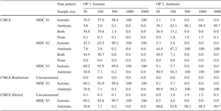
4. CMLE filtered as described in Sect.5.2.3,c˜=0.90. Table 1 shows the resulting classification of the mono-tonicity direction for each OP according to the five con-strained estimation methods discussed here. After fitting the UMLEs, the MDC procedure was performed as part of the constrained approaches. Its first, second, and third steps (‘MDC S1’, ‘MDC S2’, and ‘MDC S3’ in Table 1) cor-rectly classified OPs 1 and 2 in nearly 100% of the cases when the sample size was at least 500. For smaller sample sizes, ‘CMLE MDC S2’ showed some better results than ‘CMLE MDC S1’ as expected, and the third step allowed to finally classify OP 1 as ‘isotonic’ in 69.2% of the cases when n = 50, which rapidly increased to 92.9% whenn = 100 and improved even more for larger sample sizes. Regarding OP 2, better results were obtained even with small sample sizes.
‘CMLE Bonferroni’ performed in exactly the same way as ‘CMLE MDC S3’ because the null hypothesis of mono-tonicity was not rejected in 100% of the data sets for both OPs with αs∗ = 0.05 and for any sample size. Therefore, the monotonicity constraints were not dropped. A rejec-tion rate of approximately 5% would have been obtained for each OP if, for instance, β1 = (0.3,1.8,1.005) and β2=(−0.2,−1.5,−0.17,−2.4,−2.41)have been used as
the true parameter patterns instead of the original ones for this simulation,β1 =(0.3,1.0,1.005)andβ2 =(−0.2,−1.5, −1.55,−2.4,−2.41)whenn=500.
The results of ‘CMLE filtered’ were similar to the ones of both ‘CMLE MDC S3’ and ‘CMLE Bonferroni’. The mono-tonicity constraints were dropped in at most 1.9% of the cases, which hardly affected the final monotonicity direction classification.
In general, smaller sample sizes provide less information to any method, increasing the misclassification rate of the monotonicity direction. However, given a monotonic
asso-Table 1 Classification of monotonicity direction of 2 OPs based on five methods with 1000 simulated data sets, different sample sizes and independent covariates (%)
True pattern OP 1: Isotonic OP 2: Antitonic
Sample size 50 100 500 1000 5000 50 100 500 1000 5000 CMLE MDC S1 Isotonic 39.5 57.9 98.4 100 100 3.1 2.9 0.0 0.0 0.0 Antitonic 5.6 2.0 0.1 0.0 0.0 39.1 82.1 98.1 98.5 99.7 Both 54.8 39.8 1.4 0.0 0.0 56.9 13.2 0.0 0.0 0.0 None 0.1 0.3 0.1 0.0 0.0 0.9 1.8 1.9 1.5 0.3 MDC S2 Isotonic 47.5 65.5 99.2 100 100 5.3 5.6 0.0 0.0 0.0 Antitonic 7.6 3.8 0.2 0.0 0.0 44.8 87.2 100 100 100 Both 44.9 30.7 0.6 0.0 0.0 49.9 7.2 0.0 0.0 0.0 None 0.0 0.0 0.0 0.0 0.0 0.0 0.0 0.0 0.0 0.0 MDC S3 Isotonic 69.2 92.9 99.8 100 100 9.1 5.7 0.0 0.0 0.0 Antitonic 30.8 7.1 0.2 0.0 0.0 90.9 94.3 100 100 100
CMLE Bonferroni Unconstrained 0.0 0.0 0.0 0.0 0.0 0.0 0.0 0.0 0.0 0.0
MDC S3 Isotonic 69.2 92.9 99.8 100 100 9.1 5.7 0.0 0.0 0.0
Antitonic 30.8 7.1 0.2 0.0 0.0 90.9 94.3 100 100 100
CMLE filtered Unconstrained 0.1 0.3 0.1 0.0 0.0 0.9 1.8 1.9 1.5 0.3
MDC S3 Isotonic 69.1 92.6 99.7 100 100 8.5 4.6 0.0 0.0 0.0
Antitonic 30.8 7.1 0.2 0.0 0.0 90.6 93.6 98.1 98.5 99.7
ciation, when the value of the parameter estimate associated with the last category is further away from zero, there is less probability of misclassification irrespective of the sam-ple size. This is the case for OP 2 (see Fig.5as an example whenn=500), which was correctly classified in more than 90% of the cases by every method, even when the sample size was as small as 50.
Consider one of the 1000 data sets as an example to illustrate the case of imposing monotonicity constraints. As shown in Fig.5, some unconstrained parameter estimates are incompatible with the monotonicity assumptions. Despite the fact that the OP 1 is assumed to be isotonic, the UMLE yields
ˆ
β1,2 <0 andβˆ1,3>βˆ1,4. Similar violations occur with the
second ordinal predictor (antitonic), withβˆ2,3 < βˆ2,4. By
contrast, the results of the CMLEs imposed monotonicity constraints, with the estimate forβ1,2being greater than zero,
the estimate forβ1,4being slightly greater than the one for
β1,3, and where the estimate forβ2,4was slightly lesser than
the one forβ2,3. The monotonicity directions were
estab-lished in the first step of the MDC procedure; therefore, the methods ‘CMLE MDC S1’, ‘CMLE MDC S2’, and ‘CMLE MDC S3’ provided the same result. Similarly, the first step of the MDC procedure did not classify OPs 1 or 2 as ‘none’, and the monotonicity test did not reject the null hypothesis of monotonicity for any of these two OPs; therefore ,‘CMLE Bonferroni’ and ‘CMLE filtered’ are not shown.
In this particular example, the CMLEs for the parameter estimates associated with both intercepts and interval scale
Fig. 5 An example of unconstrained MLE and constrained MLE for a
particular data set from simulations with 2 independent OPs andn=
500
covariates were hardly affected by the monotonicity assump-tion when comparing the CMLE to the UMLE.
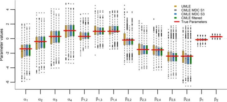
Regardless of the sample size, imposing monotonicity constraints reduces the parameter space, which affects the distribution of the parameter estimates when they are active. As an illustration, Fig.6uses boxplots to visualise the dis-tribution of each parameter estimate resulting from several methods together with the true parameters used in the data generation process for the 1000 simulation iterations with n =100.
The effect of the monotonicity constraints is depicted by the range of values that the parameter estimates take for an OP in some of the constrained approaches, which differs from the one of the UMLEs in two aspects. First, when the parameter estimates are correctly constrained, they are compatible with their monotonicity direction, i.e., they take positive values for the isotonic case and negative for the antitonic one. This
Fig. 6 Unconstrained MLE, different methods with constrained MLE and true parameters used for 1000 simulated data sets with 2 independent
OPs, example forn=100
is why the boxes of some constrained approaches seem to be truncated at zero forβ1,2andβ2,2. The second difference is
a generalisation of the first one as any constrained param-eter estimate is greater/lower than the one of the preceding category rather than greater/lower than zero only. Hence, the lower extremes of their boxplots show shorter whiskers than the ones of the UMLE when there is an isotonic relationship, and the same effect occurs for the upper whiskers when the relationship is antitonic.
The results of ‘CMLE MDC S1’ are the closest to the ones of the unconstrained method. This is due to the fact that ‘CMLE MDC S1’ drops the monotonicity constraints more frequently than any other constrained method. Conversely, ‘CMLE MDC S3’ is the furthest because it does not drop constraints. Other constrained methods are in between these two. The approaches ‘CMLE MDC S3’ and ‘CMLE Bon-ferroni’ delivered the same results because the monotonicity tests did not reject monotonicity for any OP. Compared to other constrained approaches, the results of ‘CMLE filtered’ are slightly different because there are 18 cases where the OP 2 was considered as non-monotonic and 3 for OP 1, for which the monotonicity constraints were not imposed. Unconstrained cases together with misclassification of the monotonicity direction are the reason why there are some negative values for the estimates of OP 1 and positive values for the ones of OP 2 in the constrained approaches.
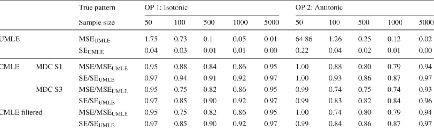
Mean square error (MSE) and the standard error (SE) of the parameter estimates are shown in Table2, averaged over all parameters belonging to an OP. The values for the constrained methods are given relative to the values for UMLE.
The constrained methods lead to a lower MSE than UMLE irrespective of the sample size. The MSE ratio of the con-strained methods with UMLE is higher for both the smallest and largest sample sizes than for the intermediate ones. For the largest sample size and given truly monotonic ordinal predictors as in this simulation, the constrained methods pro-vide results close to UMLE, because the UMLE reveals the true monotonic patterns for large enoughn. For the smallest sample size, the MSE results of the constrained methods are fairly close to UMLE because the variability of their param-eter estimates is affected by a considerable misclassification rate when imposing monotonicity constraints.
As an example of the analysis of the MSE, consider the results for n = 100 shown in Fig. 7. The total MSE is notably smaller for the constrained approaches. On aver-age, the ‘CMLE MDC S1’ shows a 10.2% smaller MSE compared to the MSE of UMLE for the intercepts , 10.7% smaller for the first ordinal predictor, and 11.2% smaller for the second. The corresponding figures for ‘CMLE MDS S3’ are 24.2%, 24.6%, and 24.9%, and for ‘CMLE filtered’ are 22.9%, 24.1%, and 24.6%.
The performance of ‘CMLE Bonferroni’ is almost identi-cal to ‘CMLE MDC S3’. The results of ‘CMLE MDC S2’ lie between those of ‘CMLE MDC S1’ and ‘CMLE MDC S3’. These are not shown in Fig.7and later.
Despite the fact that the squared bias makes a markedly small contribution to the total MSE (lighter colours in Fig.7), it is clearly higher for some constrained parameter estimates, specially for those of OP 2. Its sixth category produced the highest squared bias, which represents from 3.9% of its total MSE for ‘CMLE MDC S1’ up to 10.0% for ‘CMLE filtered’.
Table 2 Average of the MSEs and average of the SEs associated with the categories of each OP when using UMLE (MSEUMLEand SEUMLE)
True pattern OP 1: Isotonic OP 2: Antitonic
Sample size 50 100 500 1000 5000 50 100 500 1000 5000
UMLE MSEUMLE 1.75 0.73 0.1 0.05 0.01 64.86 1.26 0.25 0.12 0.02
SEUMLE 0.04 0.03 0.01 0.01 0.00 0.22 0.04 0.02 0.01 0.00
CMLE MDC S1 MSE/MSEUMLE 0.95 0.88 0.84 0.86 0.95 1.00 0.88 0.80 0.79 0.94
SE/SEUMLE 0.97 0.94 0.91 0.92 0.97 1.00 0.93 0.86 0.87 0.97
MDC S3 MSE/MSEUMLE 0.95 0.75 0.82 0.86 0.95 0.99 0.74 0.75 0.74 0.93
SE/SEUMLE 0.97 0.85 0.90 0.92 0.97 0.99 0.83 0.82 0.84 0.96
CMLE filtered MSE/MSEUMLE 0.95 0.75 0.82 0.86 0.95 1.00 0.74 0.80 0.79 0.94
SE/SEUMLE 0.97 0.85 0.90 0.92 0.97 0.99 0.84 0.86 0.87 0.97
Ratio of the average of the MSEs associated with the categories of each OP when using other methods to MSEUMLE, and ratio of the average
standard errors of a constrained method to the one of the UMLE (MSE/MSEUMLEand SE/SEUMLE). Independent covariates
Fig. 7 Mean square error for unconstrained and constrained MLEs and its decomposition, example forn=100
The squared bias of the constrained approaches associated with the remaining categories of OP 2 together with the first OP and the intercepts represent, on average, between 1.4 and 3.4% of the MSE depending on the constrained method (‘CMLE MDC S1’ being the smallest and both ‘CMLE MDC S3’ and ‘CMLE Bonferroni’ the largest). Consequently, the MSEs are dominated by variances, which are considerably lower than the ones of the UMLE not only for the parameters associated with the ordinal predictor categories, but also for the intercepts.
The simulation was repeated with dependence among covariates. In order to simulate the predictors, we generated a set of four variables from a multivariate normal distribu-tion with means equal to zero and unit variances for the two ordinal variables and the same means and variances that were used in the setting with independent covariates for the two interval scale variables. The correlation struc-ture was set allowing different magnitudes and directions as follows: ρ= ⎡ ⎢ ⎢ ⎣ 1 −0.3 0.6 0.7 −0.3 1 −0.5−0.2 0.6 −0.5 1 0.2 0.7 −0.2 0.2 1 ⎤ ⎥ ⎥ ⎦.
The categorisation of the ordinal variables resulted from clas-sifying each simulated value within the limits defined by the normal quantiles corresponding to the cumulative prob-abilities obtained from the marginal distributions that were previously set for those OPs with 4 and 6 categories (see Fig.2).
The monotonicity direction classification results obtained from the setting with correlated predictors are shown in Table 3. For sample sizes n = 50 and n = 100, there is more misclassification for OP 1 in the scenario with corre-lated covariates. For larger sample sizes (n ≥500), the final results of the setting with correlated covariates are nearly as good as the ones with independent covariates for OP 1. The
Table 3 Classification of monotonicity direction of 2 OPs based on five methods with 1000 simulated data sets, different sample sizes and correlated covariates (%)
True pattern OP 1: Isotonic OP 2: Antitonic
Sample size 50 100 500 1000 5000 50 100 500 1000 5000 CMLE MDC S1 Isotonic 25.0 35.6 87.4 98.7 100 2.9 2.3 0.0 0.0 0.0 Antitonic 5.9 2.9 0.3 0.0 0.0 27.8 61.0 97.8 98.5 100 Both 69.0 61.5 12.2 1.3 0.0 68.9 35.5 0.0 0.0 0.0 None 0.1 0.0 0.1 0.0 0.0 0.4 1.2 2.2 1.5 0.0 MDC S2 Isotonic 33.1 43.9 92.3 99.2 100 4.5 4.3 0.0 0.0 0.0 Antitonic 7.4 4.4 0.8 0.2 0.0 35.0 67.0 100 100 100 Both 59.5 51.7 6.9 0.6 0.0 60.5 28.7 0.0 0.0 0.0 None 0.0 0.0 0.0 0.0 0.0 0.0 0.0 0.0 0.0 0.0 MDC S3 Isotonic 58.5 73.7 98.9 99.8 100 9.8 5.1 0.0 0.0 0.0 Antitonic 41.5 26.3 1.1 0.2 0.0 90.2 94.9 100 100 100
CMLE Bonferroni Unconstrained 0.0 0.0 0.0 0.0 0.0 0.0 0.0 0.1 0.1 0.0
MDC S3 Isotonic 58.5 73.7 98.9 99.8 100 9.8 5.1 0.0 0.0 0.0
Antitonic 41.5 26.3 1.1 0.2 0.0 90.2 94.9 99.9 99.9 100
CMLE filtered Unconstrained 0.1 0.0 0.1 0.0 0.0 0.4 1.2 2.2 1.5 0.0
MDC S3 Isotonic 58.5 73.9 98.9 99.8 100 9.7 4.3 0.0 0.0 0.0
Antitonic 41.4 26.1 1.0 0.2 0.0 89.9 94.5 97.8 98.5 100
Table 4 Average of the MSEs and average of the SEs associated with the categories of each OP when using UMLE (MSEUMLEand SEUMLE)
True pattern OP 1: Isotonic OP 2: Antitonic
Sample size 50 100 500 1000 5000 50 100 500 1000 5000
UMLE MSEUMLE 8.68 0.84 0.14 0.08 0.01 87.62 43.63 0.28 0.14 0.02
SEUMLE 0.09 0.03 0.01 0.01 0.00 0.25 0.19 0.02 0.01 0.00
CMLE MDC S1 MSE/MSEUMLE 0.99 0.98 0.94 0.94 0.97 0.98 1.00 0.92 0.92 0.93
SE/SEUMLE 1.00 0.98 0.97 0.96 0.98 0.98 1.00 0.95 0.95 0.96
MDC S3 MSE/MSEUMLE 0.70 1.01 0.92 0.94 0.97 0.95 1.00 0.89 0.90 0.93
SE/SEUMLE 0.84 0.98 0.95 0.96 0.98 0.95 1.00 0.93 0.93 0.96
CMLE filtered MSE/MSEUMLE 0.70 1.01 0.92 0.94 0.97 0.95 1.00 0.92 0.92 0.93
SE/SEUMLE 0.84 0.98 0.95 0.96 0.98 0.95 1.00 0.95 0.95 0.96
Ratio of the average of the MSEs associated with the categories of each OP when using other methods to MSEUMLE, and ratio of the average
standard errors of a constrained method to the one of the UMLE (MSE/MSEUMLEand SE/SEUMLE). Correlated covariates
latter occurs for OP 2 also, but for any of the sample sizes, including the smallest.
Table4 shows the MSE results with correlated predic-tors. Compared to the scenario with independent covariates, the MSE of the version with correlated covariates is always higher, regardless of the sample size and method. The MSEs decrease as n increases; the magnitude of the reduction depends on the method and the sample size. For example, for ‘CMLE MDC S3’ and other highly constrained meth-ods, with correlated predictors the ratio MSE/MSEUMLE
increases for OP 1 whennchanges from 50 to 100. Despite the fact that OP 1 is often misclassified by the more restric-tive methods such as ‘CMLE MDC S3’, their MSE ratio is
still low whenn =50 because of the high variance of the UMLE, which is amended by the constrained methods.
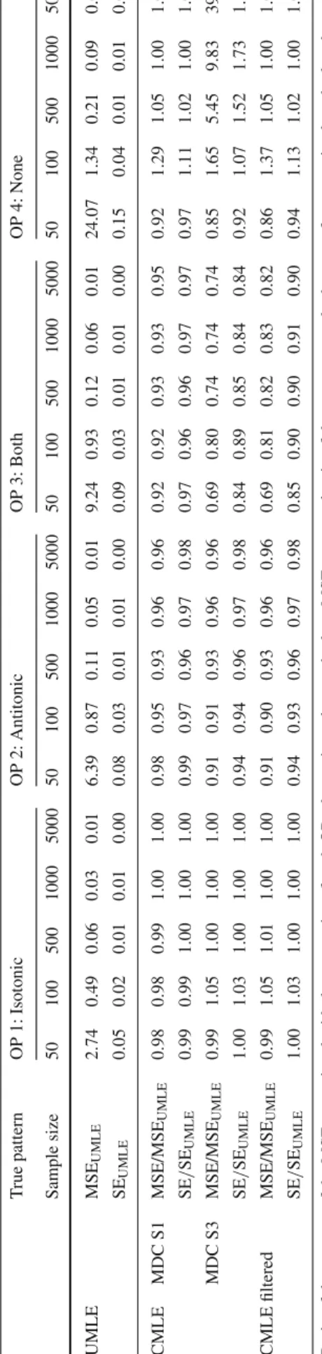
In the simulation presented above, no non-monotonic ordinal predictor was included and its results showed that any constrained approach performed better than the uncon-strained one in almost every simulated scenario. In order to analyse their performance in presence of non-monotonic OPs, consider another simulation of model (4). This time we use an ordinal response with four categories, i.e.,k=4 and j = 1,2,3; four ordinal predictors (t = 4) with p1 = 3,
p2 = 4, p3 = 5, and p4 =6 categories correspondingly;
and one interval scale predictor (v=1). Again, several sam-ple sizes were considered: n = 50,100,500,1000,5000.
Table 5 Classification o f m onotonicity direction o f 4 OPs b ased on fiv e m ethods with 1000 simulated d ata sets and independent co v ariates (%) T rue pattern OP 1: Isotonic O P 2 : A ntitonic O P 3 : B oth O P 4 : N one Sample size 50 100 500 1000 5000 50 100 500 1000 5000 50 100 500 1000 5000 50 100 500 1000 5000 CMLE MDC S 1 Isotonic 44.5 63.4 99.1 100 100 3.8 1 .1 0.0 0 .0 0.0 17.3 15.0 13.5 14.1 11.8 26.3 33.7 2 .7 0.0 0 .0 Antitonic 3 .5 0.8 0 .0 0.0 0 .0 52.6 74.7 100 100 100 19.3 16.7 11.3 13.7 11.2 23.8 21.4 0 .0 0.0 0 .0 Both 51.9 35.8 0 .9 0.0 0 .0 43.0 23.9 0 .0 0.0 0 .0 62.1 67.7 75.2 72.2 77.0 36.6 13.8 0 .0 0.0 0 .0 None 0.1 0 .0 0.0 0 .0 0.0 0 .6 0.3 0 .0 0.0 0 .0 1.3 0 .6 0.0 0 .0 0.0 13.3 31.1 97.3 100 100 MDC S 2 Isotonic 51.1 70.0 99.3 100 100 5.8 2 .3 0.0 0 .0 0.0 22.7 21.6 18.8 19.4 17.3 34.9 43.7 31.6 2 .8 0.0 Antitonic 4 .9 1.3 0 .0 0.0 0 .0 60.1 80.0 100 100 100 25.2 22.8 16.7 20.3 16.3 39.3 48.4 15.4 0 .0 0.0 Both 44.0 28.7 0 .7 0.0 0 .0 34.1 17.7 0 .0 0.0 0 .0 51.9 55.6 64.5 60.3 66.4 25.6 7 .7 0.0 0 .0 0.0 None 0.0 0 .0 0.0 0 .0 0.0 0 .0 0.0 0 .0 0.0 0 .0 0.2 0 .0 0.0 0 .0 0.0 0 .2 0.2 53.0 97.2 100 MDC S 3 Isotonic 68.8 83.4 99.7 100 100 14.0 6 .6 0.0 0 .0 0.0 41.4 44.5 29.9 21.9 17.7 48.0 49.0 64.9 81.0 98.6 Antitonic 31.2 16.6 0 .3 0.0 0 .0 86.0 93.4 100 100 100 58.6 55.5 70.1 78.1 82.3 52.0 51.0 35.1 19.0 1 .4 CMLE Bonferroni Unconstrained 0 .0 0.0 0 .0 0.0 0 .0 0.0 0 .0 0.0 0 .0 0.0 0 .1 0.0 0 .0 0.0 0 .0 0.4 1 .3 85.2 99.7 100 MDC S 3 Isotonic 68.8 83.3 99.5 100 100 14.0 6 .6 0.0 0 .0 0.0 41.5 44.4 45.6 50.0 48.6 47.9 48.9 13.8 0 .3 0.0 Antitonic 31.2 16.7 0 .5 0.0 0 .0 86.0 93.4 100 100 100 58.4 55.6 54.4 50.0 51.4 51.7 49.8 1 .0 0.0 0 .0 CMLE filtered U nconstrained 0 .1 0.0 0 .0 0.0 0 .0 0.6 0 .3 0.0 0 .0 0.0 1 .3 0.6 0 .0 0.0 0 .0 13.3 31.1 97.3 100 100 MDC S 3 Isotonic 68.2 83.5 99.6 100 100 13.1 5 .2 0.0 0 .0 0.0 40.6 42.5 48.7 50.0 48.6 45.5 41.7 2 .7 0.0 0 .0 Antitonic 31.7 16.5 0 .4 0.0 0 .0 86.3 94.5 100 100 100 58.1 56.9 51.3 50.0 51.4 41.2 27.2 0 .0 0.0 0 .0