The Cross-Section of Foreign Currency Risk Premia and Consumption Growth Risk.

NOTES D’ÉTUDES

ET DE RECHERCHE

THE CROSS-SECTION OF

FOREIGN CURRENCY RISK

PREMIA AND CONSUMPTION GROWTH RISK

August 2006

DIRECTION GÉNÉRALE DES ÉTUDES ET DES RELATIONS INTERNATIONALES

DIRECTION DE LA RECHERCHE

THE CROSS-SECTION OF

FOREIGN CURRENCY RISK

PREMIA AND CONSUMPTION GROWTH RISK

August 2006

NER - R # 155

Les Notes d'Études et de Recherche reflètent les idées personnelles de leurs auteurs et n'expriment pas nécessairement la position de la Banque de France. Ce document est disponible sur le site internet de la Banque de France « www.banque-france.fr ».

Working Papers reflect the opinions of the authors and do not necessarily express the views of the Banque de France. This document is available on the Banque de France Website “www.banque-france.fr”.

The Cross-Section of Foreign Currency Risk

Premia and Consumption Growth Risk

Hanno Lustig and Adrien Verdelhan

UCLA/NBER and Boston University/Banque de France

August 2006

∗_{First version November 2003. The authors especially thank two anonymous referees, Andy Atkeson,} John Cochrane, Lars Hansen and Anil Kashyap for detailed comments. We would also like to thank Ravi Bansal, Craig Burnside, Hal Cole, Virgine Coudert, Fran¸cois Gourio, Martin Eichenbaum, John Heaton, Patrick Kehoe, Isaac Kleshchelski, Chris Lundbladd, Lee Ohanian, Fabrizio Perri, Sergio Rebelo, Stijn Van Nieuwerburgh and seminar participants at various institutions and conferences.

Abstract: Aggregate consumption growth risk explains why low interest rate currencies do not appreciate as much as the interest rate differential and why high interest rate currencies do not depreciate as much as the interest rate differential. Domestic investors earn negative excess returns on low interest rate currency portfolios and positive excess returns on high interest rate currency portfolios. Because high interest rate currencies depreciate on average when domestic consumption growth is low and low interest rate currencies appreciate under the same conditions, low interest rate currencies provide domestic investors with a hedge against domestic aggregate consumption growth risk.

JEL codes: F31, G12. Keywords: Exchange Rates, Asset Pricing.

R´esum´e : Un investisseur domestique re¸coit un retour sur investissement en moyenne n´egatif lorsqu’il investit dans un pays o`u le taux d’int´erˆet est bas. Il re¸coit un retour sur investissement en moyenne positif lorsqu’il investit dans un pays o`u le taux d’int´erˆet est ´elev´e. Ces primes de risque sont non nulles car les pays `a taux d’int´erˆet ´elev´es (bas) ne voient pas leurs monnaies se d´epr`ecier (s’appr´ecier) d’un montant ´equivalent au diff´erentiel de taux d’int´erˆet. Les monnaies des pays `a taux d’int´erˆet ´elev´es (bas) se d´epr´ecient (s’appr´ecient) en moyenne lorsque la consommation domestique aggr´eg´ee est faible. Ainsi les pays `a taux d’int´erˆet bas offrent un m´ecanisme d’assurance contre le risque de fluctuations de la consommation, con-duisant `a un retour sur investissement en moyenne n´egatif.

Non-technical summary: When the foreign interest rate is higher than the US interest rate, risk-neutral and rational US investors should expect the foreign currency to depreciate against the dollar by the difference between the two interest rates. This way, borrowing at home and lending abroad or vice-versa produces a zero return in excess of the domestic short-term interest rate. This is known as the uncovered interest rate parity (UIP) condition, and it is violated in the data, except in the case of very high inflation currencies. In the data, higher foreign interest rates almost always predict higher excess returns for a US investor in foreign currency markets.

We show that these excess returns compensate the US investor for taking on more US consumption growth risk. High foreign interest rate currencies on average depreciate against the dollar when US consumption growth is low, while low foreign interest rate currencies do not. The textbook logic we use for any other asset can be applied to exchange rates, and it works. If an asset offers low returns when the investor’s consumption growth is low, it is risky, and the investor wants to be compensated through a positive excess return.

To uncover the link between exchange rates and consumption growth, we build portfolios of foreign currencies excess returns on the basis of the foreign interest rates, because investors know these predict excess returns. Portfolios are re-balanced every period, so the first portfolio always contains the lowest interest rate currencies and the last portfolio always contains the highest interest rate currencies. This is the key innovation in our paper. By sorting currencies into 8 portfolios, we create a large average spread of up to five hundred basis points between low and high interest rate portfolios. This spread is an order of magnitude larger than the average spread for any two given countries.

At annual frequencies, consumption growth risk explains up to eighty percent of the varia-tion in currency excess returns across these eight currency portfolios. The estimated coefficient of risk aversion is very high, and the estimated price of US consumption growth risk is about two percent per annum. Consumption growth risk can explain the risk premia in currency markets only if we are willing to entertain high levels of risk aversion, as is the case in other asset markets. In fact, currency risk seems to be priced much like equity and bond risk.

R´esum´e non technique : Lorsque le taux d’int´erˆet `a l’´etranger est sup´erieur au taux d’int´erˆet am´ericain, un investisseur am´ericain insensible au risque de change devrait anticiper que la monnaie ´etrang`ere va se d´epr´ecier vis-a-vis du dollar, d’un montant ´egal au diff´erentiel d’int´eret entre les deux pays. De cette facon, emprunter dans la monnaie de son pays et prˆeter `

a l’´etranger, et vice-versa, produirait un retour sur investissement globalement nul. Cette hypoth`ese, connue sous le nom de parit´e non couverte des taux d’int´erˆet, est rejet´ee par les donn´ees, sauf pour les cas d’hyper-inflation. Empiriquement, un taux d’int´erˆet plus ´elev´e `

a l’´etranger conduit presque toujours `a anticiper un retour sur investissement positif sur le march´e des changes, croissant avec le diff´erentiel de taux d’int´erˆet.

Nous montrons dans ce papier que ces retours sur investissement compensent l’investisseur am´ericain pour le risque macro´economique domestique inh´erent `a cet investissement. Les monnaies des pays `a taux d’int´erˆet ´elev´es se d´epr´ecient en moyenne lorsque la consommation am´ericaine aggr´eg´ee est faible, ce qui n’est pas le cas des monnaies des pays `a taux d’int´erˆet bas. Le raisonnement usuel en finance s’applique ici, et avec succ`es. Si un actif offre un retour sur investissement faible lorsque la consommation de l’investisseur est faible, cet actif est risqu´e et l’investisseur demande `a ˆetre compens´e pour ce risque, d’o`u un retour sur investissement positif en moyenne.

Pour mettre en evidence le lien entre consommation et taux de change, nous constru-isons des portefeuilles de retour sur investissements en monnaies ´etrang`eres. Les monnaies sont class´ees sur la base de leurs taux d’int´erˆet respectifs et allou´ees dans 8 portefeuilles. La r´epartition des monnaies est op´er´ee chaque periode, de telle facon que le premier portefeuille contienne toujours les monnaies des pays o`u les taux d’int´erˆet sont les plus faibles. La con-struction de ces portefeuilles repr´esente l’innovation primordiale de notre travail.

Sur donn´ees annuelles, le risque associ´e aux fluctuations de la consommation explique 80% des diff´erences de rendements moyens entre ces portefeuilles. Le risque associ´e aux fluctuations de la consommation permet d’expliquer la prime de risque sur les march´es des changes seule-ment si l’on accepte de consid´erer de forts degr´es d’aversion au risque. C’est le mˆeme cas sur d’autres march´es d’actifs, et le prix du risque de change semble en fait proche de celui estim´e sur les march´es d’actions et d’obligations.

I

Introduction

When the foreign interest rate is higher than the US interest rate, risk-neutral and rational US investors should expect the foreign currency to depreciate against the dollar by the difference between the two interest rates. This way, borrowing at home and lending abroad or vice-versa produces a zero return in excess of the US short-term interest rate. This is known as the uncovered interest rate parity (UIP) condition, and it is violated in the data, except in the case of very high inflation currencies. In the data, higher foreign interest rates almost always predict higher excess returns for a US investor in foreign currency markets.

We show that these excess returns compensate the US investor for taking on more US consumption growth risk. High foreign interest rate currencies on average depreciate against the dollar when US consumption growth is low, while low foreign interest rate currencies do not. The textbook logic we use for any other asset can be applied to exchange rates, and it works. If an asset offers low returns when the investor’s consumption growth is low, it is risky, and the investor wants to be compensated through a positive excess return.

To uncover the link between exchange rates and consumption growth, we build eight port-folios of foreign currencies excess returns on the basis of the foreign interest rates, because investors know these predict excess returns. Portfolios are re-balanced every period, so the first portfolio always contains the lowest interest rate currencies and the last portfolio always contains the highest interest rate currencies. This is the key innovation in our paper.

Over the last three decades, in empirical asset pricing, the focus has shifted from explaining individual stock returns to explaining the returns on portfolios of stocks, sorted on variables that we know predict returns (e.g. size and book-to-market).1 This procedure eliminates the diversifiable, stock-specific component of returns that is not of interest, thus producing much sharper estimates of the risk-return trade-off in equity markets. Similarly, for currencies, by sorting these into portfolios, we abstract from the currency-specific component of exchange rate changes that is not related to changes in the interest rate. This isolates the source of variation in excess returns that interests us, and it creates a large average spread of up to five hundred basis points between low and high interest rate portfolios. This spread is an order of magnitude larger than the average spread for any two given countries. As one would expect from the empirical literature on UIP, US investors earn on average negative excess returns

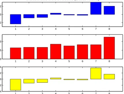
on low interest rate currencies of minus 2.3 percent and large, positive excess returns on high interest rate currencies of up to 3 percent. The relation is almost monotonic, as shown in figure 1. These returns are large even when measured per unit of risk. The Sharpe ratio (defined as the ratio of the average excess return to its standard deviation) on the high interest rate portfolio is close to 40 percent, only slightly lower than the Sharpe ratio on US equity, while the same ratio is minus 40 percent for the lowest interest rate portfolio. In addition, these portfolios keep the number of covariances that must be estimated low, while allowing us to continuously expand the number of countries studied as financial markets open up to international investors. This enables us to include data from the largest possible set of countries.

1 2 3 4 5 6 7 8

−2 0 2

Mean

Characteristics of the 8 Portfolios (Excess Returns)

1 2 3 4 5 6 7 8 0 5 10 Std 1 2 3 4 5 6 7 8 −0.4 −0.2 0 0.2 0.4 Sharpe Ratio

Figure 1: 8 Currency Portfolios.

This figure presents means, standard deviations (in percentages) and Sharpe ratios of real excess returns on 8 annually re-balanced currency portfolios for a US investor. The data are annual and the sample is 1953-2002. These portfolios were constructed by sorting currencies into eight groups at timetbased on the nominal interest rate differential with the home country at the end of periodt−1. Portfolio 1 contains currencies with the lowest interest rates. Portfolio 8 contains currencies with the highest interest rates.

To show that the excess returns on these portfolios are due to currency risk, we start from the US investor’s Euler equation and use consumption-based pricing factors. We test the model on annual data for the periods 1953-2002 and 1971-2002.

returns across these eight currency portfolios. Are the parameter estimates reasonable? Our results are not consistent with what most economists view as plausible values of risk aversion, but they are consistent with the evidence from other assets. The estimated coefficient of risk aversion is around 100, and the estimated price of US consumption growth risk is about 2 percent per annum for nondurables and 4.5 percent for durables. Consumption-based models can explain the risk premia in currency markets only if we are willing to entertain high levels of risk aversion, as is the case in other asset markets. In fact, currency risk seems to be priced much like equity risk. If we estimate the model on US domestic bond portfolios (sorted by maturity) and stock portfolios (sorted by book-to-market and size) in addition to the currency portfolios, the risk aversion estimate does not change. Our currency portfolios really allow for an ‘out-of-sample’ test of consumption-based models, because the low interest rate currency portfolios have negative average excess returns, unlike most of the test assets in the empirical asset pricing literature, and the returns on the currency portfolios are not strongly correlated with bond and stock returns.

Consumption-based models can explain the cross-section of currency excess returns if and only if high interest rate currencies typically depreciate when real US consumption growth is low, while low interest rate currencies appreciate. This is exactly the pattern we find in the data. We can restate this result in standard finance language using the consumption growth beta of a currency. The consumption growth beta of a currency measures the sensitivity of the exchange rate to changes in US consumption growth. These betas are small for low interest rate currencies and large for high interest rate currencies. In addition, for the low interest rate portfolios, the betas turn negative when the interest rate gap with the US is large. All our results build on this finding.

Section I outlines our empirical framework and defines the foreign currency excess returns and the potential pricing factors. Section II tests consumption-based models on the uncon-ditional moments of our foreign currency portfolio returns. Section III links our results to properties of exchange rate betas. Section IV checks the robustness of our estimates in various ways. Finally, section V concludes with a review of the relevant literature. Data on currency returns and the composition of the currency portfolios are available on the authors’ web sites.2

II

Foreign Currency Excess Returns

This section first defines the excess returns on foreign T-bill investments and details the con-struction and characteristics of the currency portfolios. We then turn to the US investor’s Euler equation and we explain how consumption risk can explain the average excess returns on these currency portfolios.

A

Why Build Portfolios of Currencies?

We focus on a US investor who invests in foreign T-bills or equivalent instruments. These bills are claims to a unit of foreign currency one period from today in all states of the world. R_ti₊₁ denotes the risky dollar return from buying a foreign T-bill in country i, selling it after one period and converting the proceeds back into dollars: Ri_t+1 = Ri,_t£E

i t+1 Ei t , where E i t is the

exchange rate in dollar per unit of foreign currency, Ri,_t£ is the risk-free one-period return in units of foreign currency i.3 _{We use P}

t to denote the dollar price of the US consumption

basket. Finally, R_ti,e₊₁ = R_ti₊₁−R$_t Pt

Pt+1 is the real excess return from investing in foreign

T-bills, andR$_t is the nominal risk-free rate in US currency. Below, we use lowercase symbols to denote the log of a variable.

UIP regressions and Currency Risk premia According to the UIP condition, the

slope in a regression of the change in the exchange rate for currency i on the interest rate differential is equal to one:

−∆ei_t+1 =αi₀+αi₁Ri,_t£−R$_t+ǫi_t+1,

and the constant is equal to zero. The data consistently produce slope coefficients less than one, mostly even negative.4 Of course, this immediately implies that the (nominal) expected excess returns, which are roughly equal toRi,_t£−R$_t+Et∆eit+1, are not zero and that they

are predicted by interest rates: higher interest rates predict higher excess returns.

3_{Note that returns are dated by the time they are known. Thus,R}i,£

t is the nominal risk free rate

between periodt andt+ 1, which is known at date t.

4

See Hansen and Hodrick (1980) and Fama (1984). Hodrick (1987) and Lewis (1995) provide exten-sive surveys and updated regression results.

Currency Portfolios To better analyze the risk-return trade-off for a US investor investing in foreign currency markets, we construct currency portfolios that zoom in on the predictability of excess returns by foreign interest rates.

At the end of each period t, we allocate countries to eight portfolios on the basis of the nominal interest rate differential, Ri,_t£−R$_t, observed at the end of period t. The portfolios are rebalanced every year. They are ranked from low to high interests rates, portfolio 1 being the portfolio with the lowest interest rate currencies and portfolio 8 being the one with the highest interest rate currencies. By building portfolios, we filter out currency changes that are orthogonal to changes in interest rates. LetNj denote the number of currencies in portfolioj,

and let us simply assume that currencies within a portfolio have the same UIP constant and slope coefficients. Then, for portfolioj, the change in the ‘average’ exchange rate will reflect mainly the risk premium component, αj₀+αj_1N1

j

P

i

Ri,_t£−R$_t, the part we are interested in.

We always use a total number of eight portfolios. Given the limited number of countries, especially at the start of the sample, we did not want too many portfolios. If we choose less than eight portfolios, then the currencies of countries with very high inflation end up being mixed with others. It is important to keep these currencies separate because the returns on these very high interest rate currencies are very different, as will become more apparent below. Next, we compute excess returns of foreign T-bill investmentsRj,e_t+1 for each portfolioj by averaging across the different countries in each portfolio. We useET to denote the sample mean

for a sample of sizeT. The variation in average excess returnsET

h

Rj,e_t+1iforj= 1, . . . ,8 across portfolios is much larger than the spread in average excess returns across individual currencies, because foreign interest rates fluctuate over time: the foreign excess return is positive (negative) when foreign interest rates are high (low), and periods of high excess returns are canceled out by periods of low excess returns. Our portfolios shift the focus from individual currencies to high vs. low interest rate currencies, in the same way that the Fama and French (1992) portfolios of stocks sorted on size and book-to-market ratios shift the focus from individual stocks to small/value vs. large/growth stocks.

B

Data

With these eight portfolios, we consider two different time-horizons. First, we study the period 1953 to 2002, which spans a number of different exchange rate arrangements. The Euler equation restrictions are valid regardless of the exchange rate regime. Second, we consider a shorter time period, 1971 to 2002, beginning with the demise of Bretton-Woods.

Interest Rates and Exchange Rates For each currency, the exchange rate is the end-of-month average daily exchange rate, from Global Financial Data. The foreign interest rate is the interest rate on a 3-month government security (e.g. a US T-bill) or an equivalent instrument, also from Global Financial Data. We used the 3-month interest rate instead of the one-year rate, simply because fewer governments issue bills or equivalent instruments at the one year maturity. As data became available, new countries were added to these portfolios. As a result, the composition of the portfolio as well as the number of countries in a portfolio changes from one period to the next. Section A.1 in the Appendix contains a detailed list of the currencies in our sample.

Two additional issues need to be dealt with: the existence of expected and actual default events, and the effects of financial liberalization.

Default Defaults can impact our currency returns in two ways. First, expected defaults should lead rational investors to ask for a default premium, thus increasing the foreign interest rate and the foreign currency return. To check that our results are due to currency risk, we run all experiments for a sub-sample of developed countries. None of these countries has ever defaulted, nor were they ever considered likely candidates. Yet, we obtain very similar results. Second, actual defaults modify the realized returns. To compute actual returns on an investment after default, we used the data set of defaults compiled by Reinhart, Rogoff and Savastano (2003). The (ex ante) recovery rate we applied is seventy percent. This number reflects two sources, Singh (2003) and Moody’s Investors Service (2003), presented in section A.2 of the Appendix. If a country is still in default in the following year, we simply exclude it from the sample for that year.5

5_{In the entire sample from 1953 to 2002, there are thirteen instances of default by a country whose}

currency is in one of our portfolios: Zimbabwe (1965), Jamaica (1978), Jamaica (1981), Mexico (1982), Brazil (1983), Philippines (1983), Zambia (1983), Ghana (1987), Jamaica (1987), Trinidad and Tobago

Capital Account Liberalization The restrictions imposed by the Euler equation on the joint distribution of exchange rates and interest rates only make sense if foreign investors can in fact purchase local T-bills. Quinn (1997) has built indices of openness based on the coding of the IMF Annual Report on Exchange Arrangements and Exchange Restrictions. This report covers fifty-six nations from 1950 onwards and 8 more starting in 1954-1960. Quinn (1997)’s capital account liberalization index ranges from zero to one hundred. We chose a cut-off value of 20, and we eliminate countries below the cutoff. In these countries, approval of both capital payments and receipts are rare, or the payments and receipts are at best only infrequently granted.

C

Summary Statistics for the Currency Portfolio Returns

This section present some preliminary evidence on the currency portfolio returns.

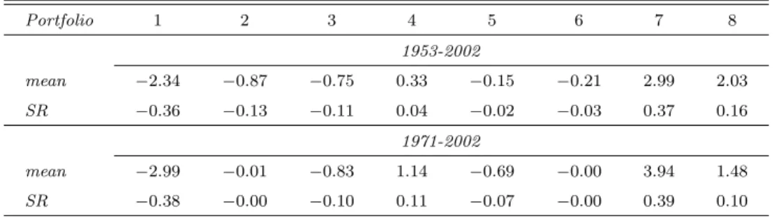
Table 1: US Investor’s Excess Returns

Portfolio 1 2 3 4 5 6 7 8 1953-2002 mean −2.34 −0.87 −0.75 0.33 −0.15 −0.21 2.99 2.03 SR −0.36 −0.13 −0.11 0.04 −0.02 −0.03 0.37 0.16 1971-2002 mean −2.99 −0.01 −0.83 1.14 −0.69 −0.00 3.94 1.48 SR −0.38 −0.00 −0.10 0.11 −0.07 −0.00 0.39 0.10

Notes: This table reports the mean of the real excess returns (in percentage points) and the Sharpe Ratio (SR) for a US investor. The portfolios are constructed by sorting currencies into eight groups at timetbased on the nominal interest rate differential at the end of periodt−1. Portfolio 1 contains currencies with the lowest interest rates. Portfolio 8 contains currencies with the highest interest rates. The table reports annual returns for annually re-balanced portfolios.

The first panel of table 1 lists the average excess return in units of US consumption ET

h

Rj,e_t+1i and the Sharpe ratio for each of the annually re-balanced portfolios. The largest spread (between the first and the seventh portfolio) exceeds five percentage points for the entire sample, and close to seven percentage points in the shorter sub-sample. The average annual returns are almost monotonically increasing in the interest rate differential. The only (1988), South Africa (1989, 1993) and Pakistan (1998). Of course, many more countries actually defaulted over this sample, but those are not in our portfolios because they imposed capital controls, as explained in the next paragraph.

exception is the last portfolio, which consists of very high inflation currencies: the average interest rate gap with the US for the eighth portfolio is about 16 percentage points over the entire sample and 23 percentage points post-Bretton Woods. As Bansal and Dahlquist (2000) have documented, UIP tends to work best at high inflation levels.

Countries change portfolios frequently (23 percent of the time), and the time-varying com-position of the portfolios is critical. If we allocate currencies into portfolios based on the average interest rate differential over the entire sample instead, then there is essentially no pattern in average excess returns.

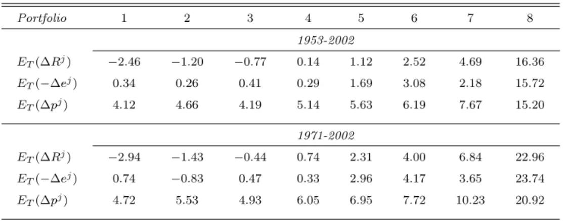
Table 2: Exchange Rates and Interest Rates

Portfolio 1 2 3 4 5 6 7 8 1953-2002 ET(∆Rj) −2.46 −1.20 −0.77 0.14 1.12 2.52 4.69 16.36 ET(−∆ej) 0.34 0.26 0.41 0.29 1.69 3.08 2.18 15.72 ET(∆pj) 4.12 4.66 4.19 5.14 5.63 6.19 7.67 15.20 1971-2002 ET(∆Rj) −2.94 −1.43 −0.44 0.74 2.31 4.00 6.84 22.96 ET(−∆ej) 0.74 −0.83 0.47 0.33 2.96 4.17 3.65 23.74 ET(∆pj) 4.72 5.53 4.93 6.05 6.95 7.72 10.23 20.92

Notes: This table reports the time-series average of the average interest rate differential ∆Rjt (in percentage points), the

average rate of depreciation (in percentage points) ∆ejt+1and the average inflation rate ∆pj(in percentage points) for

each of the portfolios. Portfolio 1 contains currencies with the lowest interest rates. Portfolio 8 contains currencies with the highest interest rates. This table reports annual interest rates, exchange rate changes and inflation rates for annually re-balanced portfolios.

Exchange Rates and Interest Rates Table 2 decomposes the average excess returns on each portfolio into its two components. For each portfolio, we report the average interest rate gap (ET(∆Rj)) in the first row of each panel in Table 2 and the average rate of depreciation

(ET(−∆ej)) in the second row.6 If there is no average risk premium, these should be identical.

Table 2 shows they are not. Investors earn large negative excess returns on the first portfolio

6_∆Rj

t is the average interest rate differential

1 Nj P i Ri,t£−R $ t

for portfolio j at time t. The average risk premium is approximately equal to the difference between the first and the second row. This approximation does not exactly lead to the excess return reported in Table 1, because Table 1 reports the real excess return (based on the real return on currency and the real US risk-free rate), and because of the log approximation.

because the low interest rate currencies in the first portfolio depreciate on average by 34 basis points, while the average foreign interest rate is 2.46 percentage points lower then the US interest rate. On the other hand, the higher interest rate currencies in the seventh portfolio depreciate on average by almost 2.18 percentage points, but the average interest rate difference is on average 4.7 percentage points. The third row in each panel reports the inflation rates. As advertised, for the very high interest rate currencies in the last portfolio, much of the interest rate gap reflects inflation differences. This is not the case for low interest rate portfolios.

Our currency portfolios create a stable set of excess returns. In order to explain the variation in these currency excess returns, we use consumption-based pricing kernels.

D

US Investor’s Euler Equation

We turn now to a description of the US investor preferences. We use Mt+1 to denote the US

investor’s real stochastic discount factor (SDF) or intertemporal marginal rate of substitution, in the sense of Hansen and Jagannathan (1991). This discount factor prices payoffs in units of US consumption. In the absence of short-sale constraints or other frictions, the US investor’s Euler equation for foreign currency investments holds for each currency i and thus for each portfolioj: (1) Et h Mt+1Rj,et+1 i = 0.

Preferences Our consumption-based asset pricing model is derived in a standard repre-sentative agent setting, following Lucas (1978) and Breeden (1979), and its extension to non-expected utility by Epstein and Zin (1989) and to durable goods by Dunn and Singleton (1986) and Eichenbaum and Hansen (1990). We adopt Yogo (2006)’s setup which conveniently nests all these models. The stand-in household has preferences over non-durable consumption Ct

and durable consumption services Dt. Following Yogo (2006), the stand-in household ranks

stochastic streams of non-durable and durable consumption{Ct, Dt}according to the following

utility index: Ut= (1−δ)u(Ct, Dt)1− 1 σ +δE_t h U_t1₊₁−γi 1 κ 1/(1−1_σ) ,

where κ = (1−γ)/(1−1/σ). δ is the subjective time discount factor, γ > 0 governs the household’s risk aversion and σ >0 is the elasticity of intertemporal substitution (EIS). The

one-period utility kernel is given by a CES-function overC and D: u(C, D) =h(1−α)C1−1ρ _+αD1− 1 ρ i1/(1−1_ρ) ,

α ∈ (0,1) is the weight on durable consumption and ρ ≥ 0 is the intratemporal elasticity of substitution between non-durables and durables. Yogo (2006)’s model, which we refer to as the EZ−DCAP M, nests four familiar models. Table 3 lists all of these. On the one hand, if we imposeγ = 1/σ , the Durable Consumption-CAPM (DCAPM) obtains, while imposingρ=σ produces the Epstein-Zin Consumption-CAPM (EZ-CCAPM). Whenγ = 1/σ and ρ=σ, the standard Breeden-LucasCCAPM obtains.

Table 3: Nested Models

Parameters CCAPM DCAPM EZ-CCAPM CAPM

γ 1/σ 1/σ

σ ρ ρ σ=ρ→ ∞

Linear Factor Model Loadings

bc γ γ+α(1/ρ−γ) κ/σ 0

bd 0 κα(1/σ−1/ρ) 0 0

bm 0 0 1−κ γ

Notes: γis the coefficient of risk aversion,ρis the intratemporal elasticity of substitution between non-durablesC and durablesDconsumption,σis the elasticity of intertemporal substitution,κ= (1−γ)/(1−1/σ).

As shown by Yogo (2006), the intertemporal marginal rate of substitution (IMRS) of the stand-in agent is given by:

(2) Mt+1 = " δ Ct+1 Ct −1_σ v(Dt+1/Ct+1) v(Dt/Ct) 1/ρ−1/σ (Rw_t+1)1−1/κ #κ ,

whereRw is the return on the market portfolio and v is defined as:

v(D/C) = " 1−α+α D C 1−1/ρ#1/(1−1ρ) .

E

Calibration

We start off by feeding actual consumption and return data into a calibrated version of our model, and we assess how much of the variation in currency excess returns this calibrated model can account for. To do so, we take Yogo (2006)’s estimates of the substitution elasticities and the durable consumption weight in the utility function.7 Next, we feed the data for Ct, Dt

and Rw

t, the market return into the SDF in 2, and we simply evaluate the pricing errors

ET

h

Mt+1Rj,et+1 i

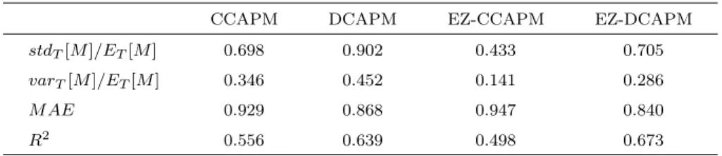
for each portfolioj. γ was chosen to minimize the mean squared pricing error on the 8 currency portfolios.8 _{Table 4 reports the implied maximum Sharpe ratio (first row),}

the market price of risk (row 2), the standard error (row 3), the mean absolute pricing error (MAE, in row 4), as well as the R2_{. The benchmark model in the last column explains 65}

% of the cross-sectional variation with γ equal to 30. To understand this result, it helps to decompose the model’s predicted excess return on currency portfolioj in the price of risk and the risk beta:

ET(Rj,et+1) = −covT[Mt+1, Rj,et+1] varT[Mt+1] | {z } β_Mj varT[Mt+1] ET[Mt+1] | {z } price of risk .

There is a large difference in risk exposure between the first and the seventh portfolios: β1

M is

-2.54, whileβ_M7 is 8.21. When multiplied by the price of risk of 28 basis points, this translates into a 3 percentage point spread in the predicted excess return between the first and the seventh portfolio, about 65 % of the actual spread. The low interest rate portfolio provides the US investor with protection against high marginal utility growth, or highM, states of the world, while the high interest rate portfolios do not. This variation in betas is the focus of the next section.

7_{We fix σat .023,αat .802 andρat .700. These parameters were estimated from a US investor’s}

Euler equation on a large number of equity portfolios (Yogo (2006), p. 552, Table II,All Portfolios).

8_{As a result of these high levels of risk aversion in a growing economy, our model cannot match the}

Table 4: Calibrated Non-Linear Model tested on 8 Currency Portfolios sorted on Interest Rates

CCAPM DCAPM EZ-CCAPM EZ-DCAPM

stdT[M]/ET[M] 0.698 0.902 0.433 0.705

varT[M]/ET[M] 0.346 0.452 0.141 0.286

M AE 0.929 0.868 0.947 0.840

R2 _{0.556 0.639 0.498 0.673}

Notes:This table reports the risk prices and the measures of fit for a calibrated model on 8 annually re-balanced currency portfolios. The sample is 1953-2002 (annual data). The first two rows report the maximum Sharpe ratio (row 1) and the price of risk (row 2). The last two rows report the mean absolute pricing error (in percentage points) and theR2_.

Following Yogo (2006), we fixedσat .023 (EZ-CCAPM andEZ-DCAPM),αat .802 (DCAPM andEZ-DCAPM) and

ρat .700 (DCAPM,EZ-DCAPM).γis fixed at 30.34 to minimize the mean squared pricing error in theEZ-DCAPM.δ

is set to .98.

III

Does Consumption Risk Explain Foreign

Cur-rency Excess Returns?

So far, we have engineered a large cross-sectional spread in currency excess returns by sorting currencies into portfolios, and we have shown that a calibrated version of the model explains a large fraction of this spread. In this section, starting from the Euler equation and following Yogo (2006), we derive a linear factor model whose factors are non-durable US consumption growth ∆ct, durable US consumption growth ∆dt and the log of the US market return rmt .

Using standard linear regression methods, we show that US consumption risk explains most of the variation in average excess returns across the eight currency portfolios, because on average low interest rate currencies expose US investors to less non-durable and durable consumption risk than high interest rate currencies. We start by deriving the factor model, then we describe the estimation method and we present our results in terms of fit, factor prices and preference parameters.

A

Linear Factor Model

The US investor’s unconditional Euler equation (approximately) implies a linear three-factor model for the expected excess return on portfolioj:9

(3) E[Rj,e] =b1cov ∆ct, Rj,et +b2cov ∆dt, Rj,et +b3cov rw_t, Rj,e_t+1. The vector of factor loadings bdepend on the preference parameters σ, αand ρ:

(4) b=     κ[1/σ+α(1/ρ−1/σ)] κα(1/σ−1/ρ) 1−κ    .

The expected excess return on portfolioj is governed by the covariance of its returns with non-durable consumption growth, durable consumption growth and the market return. When b1 > 0 (the case that obtains when γ > 1 and σ < 1), then an asset with high non-durable

consumption growth beta must have a high expected excess return. This turns out to be the empirically relevant case. b2 > 0 obtains when the intratemporal elasticity of substitution is

larger than the EIS. In this case, an asset with a high durable consumption growth beta also has a high expected excess return. In this range of the parameter space, nondurables and durables are good substitutes, and as a result, high durable consumption can offset the effect of low nondurable consumption on marginal utility.

Our benchmark asset pricing model, denoted EZ-DCAPM, is described by equation (3). This specification however nests the CCAPM with ∆ct as the only factor, theDCAPM with

∆ctand ∆dt as factors, theEZ-CCAPM, with ∆ct and rwt , and, finally theCAPM as special

cases, as shown in the bottom panel of Table 3.

Beta Representation This linear factor model can be restated as a beta pricing model, where the expected excess return is equal to the factor priceλtimes the amount of risk of each

9_{This linear factor model is derived by using a linear approximation of the SDF M}

t+1 around its

unconditional mean:

Mt+1

E[Mt+1]

≃1 +mt+1−E[mt+1],

where lower letters denote logs. Since we use excess returns, we normalize the constant in the SDF to 1, because we cannot identify it from the estimation.

portfolioβj:

(5) E[Rj,e] =λ′βj,

whereλ= Σf fband Σf f =E(ft−µf)(ft−µf)′is the variance-covariance matrix of the factors.

A Simple Example A simple example will help to understand what is needed for con-sumption growth risk to explain the cross-section of currency returns. Let us start with the plain-vanilla CCAPM. The only asset pricing factor is aggregate, non-durable consumption growth, ∆ct+1, and the factor loadingb1equals the coefficient of risk aversionγ. We can restate

the expected excess return on portfoliojas the product of the portfolio betaβcj = cov(∆ct,R

j,e t )

var(∆ct) and the factor priceλc =b1var(∆ct):

E[Rj,e_t ] = cov(∆ct, R j,e t ) var(∆ct) b1var(∆ct) =βcjλc, j= 1. . .8. (6)

The factor price measures the expected excess return on an asset that has a consumption growth beta of one. Of course, the CCAPM can explain the variation in returns only if the consumption betas are small/negative for low interest rate portfolios and large/positive for high interest rate portfolios. Essentially, in testing the CCAPM, we gauge how much of the variation in average returns across currency portfolios can be explained by variation in the consumption betas. If the predicted excess returns - the right hand side variable in equation (5) - line up with the realized sample means, then we can claim success in explaining exchange rate changes, conditional on whether the currency is a low or high interest rate currency. A key question then is whether there is enough variation in the consumption betas of these currency portfolios to explain the variation in excess returns with a plausible price of consumption risk. The next section provides a positive answer to this question.

B

An Asset Pricing Experiment

To estimate the factor prices λand the portfolio betas, we use a 2-stage procedure following Fama and MacBeth (1973).10 _{In the first stage, for each portfolio j, we run a time-series}

10_{Chapter 12 of Cochrane (2001) describes this estimation procedure and compares it to the}

regression of the currency returnsR_tj,e₊₁ on a constant and the factorsft, in order to estimate

βj. In the second stage, we run a cross-sectional regression of the average excess returnsET[Ret]

on the betas that were estimated in the first stage, to estimate the factor pricesλ. Finally, we can back out the factor loadingsb and hence the structural parameters from the factor prices.

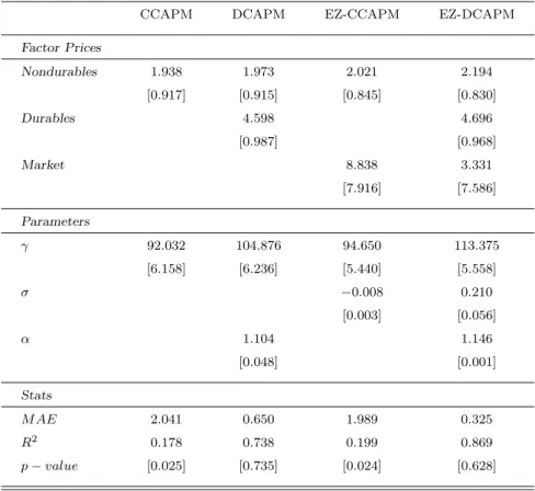
We start by testing the consumption-based US investor’s Euler equation on the eight annu-ally re-balanced currency portfolios. Table 5 reports the estimated factor prices of consumption growth risk for nondurables (row 1), for durables (row 2) and the price of market risk (row 3). Each column looks at a diferent model. We also report the implied estimates for the preference parameters γ,σ and α (rows 4-6). The standard errors are in parentheses.11 _{Finally, the last}

three rows report the mean absolute pricing error (M AE), the R2 and the p-value for a χ2 test. The null for the χ2 _{test is that the true pricing errors are zero and the p-value reports}

the probability that these pricing errors would have been observed if the consumption-based model was the true model.

C

Results

We present results in terms of the factor prices, the fit, the preference parameters and the consumption betas.

Factor Prices In our benchmark model (EZ-DCAPM), reported in the last column of Table 5, the estimated price of nondurable consumption growth risk λc is positive and statistically

significant. An asset with a consumption growth beta of one yields an average risk premium of around 2 percent per annum. This is a large number, but it is quite close to the market price of consumption growth risk estimated on US equity and bond portfolios (see section IV-C.) The estimated price of durable consumption growth riskλd is positive and statistically significant

as well. It is around 4.6 percent. These factor price estimates do not vary much across the different models. Finally, market risk is priced at about 3.3 percent per annum, but it is not significantly different from zero.

results obtained with GMM as a robustness check in section V.

11

These standard errors do not correct for the fact that the betas are estimated. Jagannathan and Wang (1996) show that the Fama-MacBeth procedure does not necessarily overstate the precision of the standard errors if conditional heteroskedasticity is present. We show in section IV - E that these standard errors are actually close to the heteroskedasticy-consistent ones derived from GMM estimates.

Model Fit We find that consumption growth risk explains a large share of the cross-sectional variation in currency returns. The EZ-DCAPM explains 87 percent of the cross-sectional variation in annual returns on the eight currency portfolios, against 74 percent for theDCAPM and 18 percent for the simpleCCAPM. For theEZ-DCAPM, the mean absolute pricing error on these eight currency portfolios is about 32 basis points over the entire sample, compared to 65 basis points for theDCAPM, and 200 basis points for the simpleCCAPM. This last number is rather high, mainly because of the last portfolio, with very high interest rate currencies. When we drop the last portfolio, the mean absolute pricing error on the remaining seven portfolios drops to 109 basis points for the simpleCCAPM, and the R2 increases to 50 percent.

The simpleCCAPM and theEZ-CCAPM are rejected at the 5 percent significance levels, but the DCAPM and the EZ-DCAPM are not. Durable consumption risk plays a key role here as the models with durable consumption growth produce very small pricing errors (less than 15 basis points) on the first and the seventh portfolio. This is clear from figure 2, which plots the actual excess return against the predicted excess return (on the horizontal axis) for each of these models.

−3 −2 −1 0 1 2 3 −3 −2 −1 0 1 2 3 CCAPM 1 2 3 4 5 6 7 8 −3 −2 −1 0 1 2 3 −3 −2 −1 0 1 2 3 DCAPM 1 2 3 4 5 6 7 8 −3 −2 −1 0 1 2 3 −3 −2 −1 0 1 2 3 EZ−CCAPM 1 2 3 4 5 6 7 8 −3 −2 −1 0 1 2 3 −3 −2 −1 0 1 2 3 EZ−DCAPM 1 2 3 4 5 6 7 8 Figure 2: Consumption-CAPM

This figure plots the actual vs. the predicted excess returns for 8 currency portfolios. The predicted excess returns are on the horizontal axis. The Fama-MacBeth estimates are obtained using 8 currency portfolios sorted on interest rates as as test assets. The filled dots (1-8) represent the currency portfolios. The data are annual and the sample is 1953-2002.

Preference Parameters and Equity Premium Puzzle ¿From the factor prices, we

Table 5: Estimation of Linear Factor Models with 8 Currency Portfolios sorted on Interest Rates

CCAPM DCAPM EZ-CCAPM EZ-DCAPM

Factor Prices Nondurables 1.938 1.973 2.021 2.194 [0.917] [0.915] [0.845] [0.830] Durables 4.598 4.696 [0.987] [0.968] Market 8.838 3.331 [7.916] [7.586] Parameters γ 92.032 104.876 94.650 113.375 [6.158] [6.236] [5.440] [5.558] σ −0.008 0.210 [0.003] [0.056] α 1.104 1.146 [0.048] [0.001] Stats M AE 2.041 0.650 1.989 0.325 R2 _{0.178 0.738 0.199 0.869} p−value [0.025] [0.735] [0.024] [0.628]

Notes: This table reports the Fama-MacBeth estimates of the risk prices (in percentage points) using 8 annually re-balanced currency portfolios as test assets. The sample is 1953-2002 (annual data). The factors are demeaned. The standard errors are reported between brackets. The last three rows report the mean absolute pricing error (in percentage points), theR2 _{and the p-value for aχ}2 _test.

non-durables and durables ρ cannot be separately identified from the weight on durable con-sumptionα. We use Yogo (2006)’s estimate ofρ=.790 to calibrate the elasticity of intratem-poral substitution when we back out the other preference parameter estimates. The EIS σ is estimated to be .2, substantially larger than 1/γ, and the weight on durable consumption α is estimated to be around 1.1, close to the .9 estimate reported by Yogo (2006), obtained on quarterly equity portfolios. Since the EIS estimate is significantly smaller than the calibrated ρ, marginal utility growth decreases in durable consumption growth, and assets whose returns co-vary more with durable consumption growth trade at a discount (b2 >0).

In the benchmark model, the implied coefficient of risk aversion is around 114 and this estimate is quite precise. In addition, these estimates do not very much across the four different

Table 6: Estimation of Factor Betas for 8 Currency Portfolios sorted on Interest Rates P ortf olios 1 2 3 4 5 6 7 8 Panel A: 1953-2002 Non-durables 0.105 0.762 0.263 0.182 0.634 0.260 1.100 0.085 Durables 0.240 0.489 0.636 0.892 0.550 0.695 1.298∗ _0.675 Market −0.066∗ _{−0.027 −0.012 −0.119}∗ _{−0.000 −0.012 −0.056 0.028} Panel B: 1971-2002 Non-durables 0.005 0.896 0.359 0.665 0.698 0.319 1.546 −0.461 Durables 0.537 0.786 1.288∗ _2.032∗ _1.225∗ _{1.359 2.183}∗ _0.845 Market −0.106∗ _−0.099∗ _{−0.026 −0.171}∗ _{−0.017 −0.007 −0.083 0.052}

Notes: Each column of this table reports OLS estimates of βj _{in the following time-series regression of excess returns}

on the factor for each portfolioj: Rj,et+1=β

j

0+β

j

1ft+ǫjt+1.The estimates are based on annual data. Panel A reports

results for 1953-2002 and Panel B reports results for 1971-2002. We use 8 annually re-balanced currency portfolios sorted on interest rates as test assets. ∗indicates significance at 5% level. We use Newey-West heteroskedasticity-consistent standard errors with an optimal number of lags to estimate the spectral density matrix following Andrews (1991).

specifications of the consumption-based pricing kernel. This coefficient of risk aversion is of course very high, but it is in line with stock-based estimates of the coefficient of risk aversion found in the literature, and with our own estimates based on bond and stock returns. For example, if we re-estimate the model only on the 25 Fama-French equity portfolios, sorted on size and book-to market, the risk aversion estimate is 115 (with a standard error of 4.5). In addition, the linear approximation we adopted causes an underestimate of the market price of consumption risk for a given risk aversion parameterγ.

These high estimates are not surprising. The standard deviation of US consumption growth (per annum) is only 1.50 percent in our sample. This is Mehra and Prescott (1985)’s equity premium puzzle in disguise; there is not enough aggregate consumption growth risk in the data to explain the level of risk compensation in currency markets at low levels of risk aversion, as is the case in equity markets, but there is enough variation across portfolios in consumption betas to explain the spread, if the risk aversion is large enough to match the levels. We now focus on this cross-section of consumption betas.

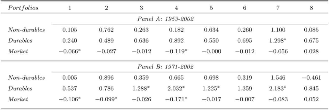
Consumption Betas Consumption-based models can account for the cross-section of cur-rency excess returns because they imply a large cross-section of betas. On average, higher interest rate portfolios expose US investors to much more US consumption growth risk. Table

6 reports the OLS betas for each of the factors. Panel A reports the results for the entire sample. We find that high interest rate currency returns are strongly pro-cyclical, while low interest rate currency returns are a-cyclical. For nondurables, the first portfolio’s consump-tion beta is 10 basis points, the seventh portfolio’s consumpconsump-tion beta is 110 basis points. For durables, the spread is also about 100 basis points, from 24 basis points to 129 basis points. In the second post-Bretton-Woods sub-sample, reported in Panel B, the spread in consumption betas increases to 150 basis points between the first and the seventh portfolio (with betas ranging from zero basis points to 154 basis points for non-durables, and from 50 to 210 basis points for durables). Finally, the market betas of currency returns are much smaller overall.

Next, we estimate the conditional factor betas, conditioning on the interest rate gap with the US, and we find that low interest rate currencies provide a consumption hedge for US investors exactly when US interest rates are high and foreign interest rates are low.

D

Conditional Factor Betas

We can go one step further in our understanding of exchange rates by taking into account the time-variation in the conditional consumption growth betas.12 It turns out that low interest rate currencies offer a consumption hedge to US investors exactly when the US interest rates are high and foreign interest rates are low. To see this, we consider a simple two-step procedure. We first obtain the U.I.P residuals ǫj_t+1 for each portfolioj. We then regress each residual on each factor fk_{, controlling for the interest rates variations in each portfolio:}

ǫj_t+1 =θj,k₀ +θ₁j,kf_tk₊₁+θ₂j,k∆Rej_tf_tk₊₁+η_tj,k₊₁,

where for expositional purpose we introduce the normalized interest rate difference ∆Rei

t, which

is zero when the interest rate difference ∆Ri_t is at a minimum and hence positive in the entire sample. We use the interest rate differential as the sole conditioning variable, because we know from the work by Meese and Rogoff (1983) that our ability to predict exchange rates is rather

12_{There is a conditional analogue of the three-factor model in equation (3):}

Et[Ri,e] =b1covt ∆ct+1, Ri,et+1 +b2covt ∆dt+1, Ri,et+1 +b3covt rw t+1, R i,e t+1 .

Since the interest rate is known att, these covariances terms involve only the changes in the exchange rate ∆ei

limited.

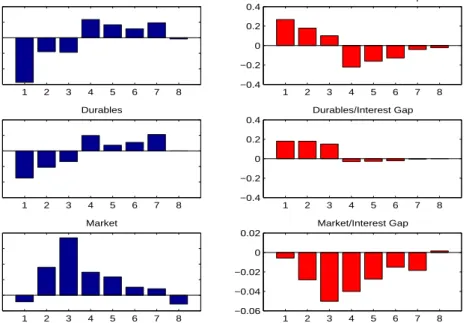
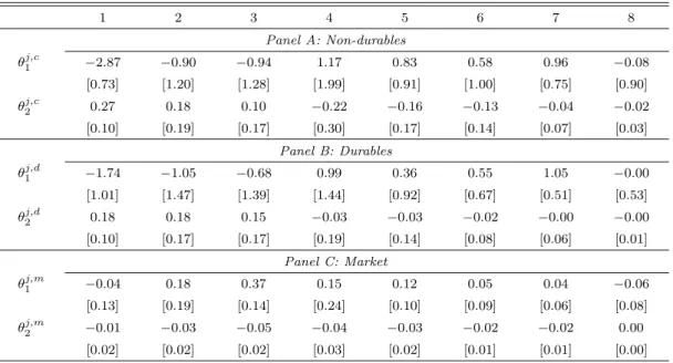
The results are reported in Table 7. Each bar in figure 3 reports the conditional factor betas for a different portfolio. The first panel reports the nondurable consumption betas, the second panel the durable consumption betas, the third panel reports the market betas. When the interest rate difference with the US hits the lowest point, the currencies in the first portfolio appreciate on average by 287 basis points when US non-durable consumption growth drops 100 basis points below its mean, while the currencies in the seventh portfolio depreciate on average by 96 basis points. Similarly, when US durable consumption growth drops 100 basis points below its mean, the currencies in the first portfolio appreciate by 174 basis points, while the currencies in the seventh portfolio depreciate by 105 basis points. Low interest rate currencies provide consumption insurance to US investors, while high interest rate currencies expose US investors to more consumption risk. As the interest rate gap closes on the currencies in the first portfolio, the low interest rate currencies provide less consumption insurance. For every 4 percentage points reduction in the interest rate gap, the non-durable consumption betas decrease by about 100 basis points.13

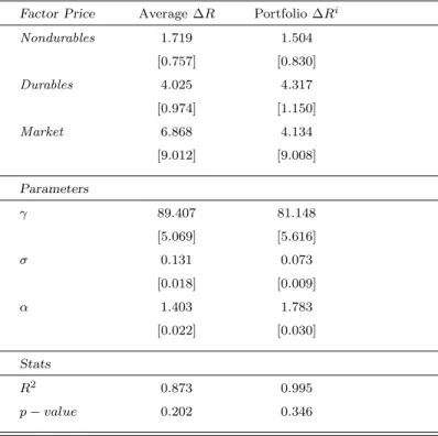
Interest rates as Instruments To test whether the representative agent’s IMRS can indeed explain the time variation in expected returns on these portfolios, in addition to the cross-sectional variation, we use the average interest rate difference with the US as an in-strument. As is clear from the unconditional Euler equation, this is equivalent to testing the unconditional moments of managed portfolio returns:

(7) EhMt+1(∆RetRi,et+1)

i

= 0,

where ∆Rt is the average interest rate difference on portfolios 1-7 and (∆RetRi,e_t+1) are the

managed portfolio returns. We normalized ∆Ret to be positive.14 Instead of the variation in

average portfolio returns, we check whether the model explains the cross-sectional variation in average excess returns onmanaged portfolios that lever up when the interest rate gap with the US is large. In addition, we also use the interest rate difference for each portfolio as an instrument for that asset’s Euler equation.

13_{This table also shows our asset pricing results are entirely driven by how exchange rates respond}

to consumption growth shocks in the US, not by sovereign risk.

14

1 2 3 4 5 6 7 8 −3 −2 −1 0 1 2 Nondurables 1 2 3 4 5 6 7 8 −0.4 −0.2 0 0.2 0.4 Nondurables/Interest Gap 1 2 3 4 5 6 7 8 −3 −2 −1 0 1 2 Durables 1 2 3 4 5 6 7 8 −0.4 −0.2 0 0.2 0.4 Durables/Interest Gap 1 2 3 4 5 6 7 8 −0.1 0 0.1 0.2 0.3 Market 1 2 3 4 5 6 7 8 −0.06 −0.04 −0.02 0 0.02 Market/Interest Gap

Figure 3: Conditional Factor Betas of Currency Each panel shows OLS estimates ofθj,k1 (panels on the left) andθ

j,k

2 (panels on the right) in the following time-series

regression of innovations to changes in exchange rate for each portfolioj on the factor and the interest rate difference interacted with the factor: ǫj_t+1=θ

j,k 0 +θ j,k 1 ftk+1+θ j,k 2 ∆Re j tftk+1+η j,k

t+1.∆Rej is the normalized interest rate difference on portfolioj. The data are annual and the sample is 1953-2002.

Table 8 reports the Fama-MacBeth estimates of the factor prices and preference parameters for our benchmark model. In the first column, we use the average interest rate difference with the US as an instrument. In the second column, we use the interest rate difference for portfolio ias an instrument for thei-th moment. The consumption risk price estimates are very close to those we obtained off the unconditional moments of currency returns, and, more importantly, the benchmark model cannot be rejected in either case.

Consumption-based models do a remarkable job in explaining the cross-sectional variation as well as the time variation in returns, albeit at the cost of a very high implied price of aggregate consumption risk. In section IV, we contrast this model’s performance with that of the workhorse of modern finance, the Capital Asset Pricing Model. As we show, there is not enough variation in market betas to explain currency returns, but there is enough variation in consumption betas. We conclude that consumption growth risk seems to play a key role in explaining currency risk premia. The next section links our findings about risk premia back to

Table 7: Estimation of Conditional Consumption Betas for Changes in Exchange Rates on Currency Portfolios Sorted on Interest Rates

1 2 3 4 5 6 7 8 Panel A: Non-durables θj,c1 −2.87 −0.90 −0.94 1.17 0.83 0.58 0.96 −0.08 [0.73] [1.20] [1.28] [1.99] [0.91] [1.00] [0.75] [0.90] θj,c2 0.27 0.18 0.10 −0.22 −0.16 −0.13 −0.04 −0.02 [0.10] [0.19] [0.17] [0.30] [0.17] [0.14] [0.07] [0.03] Panel B: Durables θj,d1 −1.74 −1.05 −0.68 0.99 0.36 0.55 1.05 −0.00 [1.01] [1.47] [1.39] [1.44] [0.92] [0.67] [0.51] [0.53] θj,d2 0.18 0.18 0.15 −0.03 −0.03 −0.02 −0.00 −0.00 [0.10] [0.17] [0.17] [0.19] [0.14] [0.08] [0.06] [0.01] Panel C: Market θj,m1 −0.04 0.18 0.37 0.15 0.12 0.05 0.04 −0.06 [0.13] [0.19] [0.14] [0.24] [0.10] [0.09] [0.06] [0.08] θj,m2 −0.01 −0.03 −0.05 −0.04 −0.03 −0.02 −0.02 0.00 [0.02] [0.02] [0.02] [0.03] [0.02] [0.01] [0.01] [0.00]

Notes: Each column of this table reports OLS estimates ofθj,k_{in the following time-series regression of innovations to}

returns for each portfolioj (ǫjt+1) on the factorfk and the interest rate difference interacted with the factor: ǫ

j t+1 = θj,k0 +θ j,k 1 ftk+1+θ j,k 2 ∆Re j tftk+1+η j,k

t+1. We normalized the interest rate difference ∆Re

j

t to be zero when the interest

rate difference ∆Rjt is at a minimum and hence positive in the entire sample. ǫ j

t+1are the residuals from the time series

regression of changes in the exchange rate on the interest rate difference (UIP regression):E_tj+1/E

j t =φ j 0+φ j 1∆R j t+ǫ j t+1.

The estimates are based on annual data and the sample is 1953-2002. We use 8 annually re-balanced currency portfolios sorted on interest rates as test assets. The pricing factors are consumption growth rates in non-durables (c) and durables (d) and the market return (w). The Newey-West heteroskedasticity-consistent standard errors computed with an optimal number of lags to estimate the spectral density matrix following Andrews (1991) are reported in brackets.

changes in the exchange rates.

IV

Mechanism

We have shown that predicted currency excess returns line up with realized ones when pricing factors take into account consumption growth risk. This is not mere luck on our part. The next section provides many robustness checks. This section sheds some light on the underly-ing mechanism: where do these currency betas come from?. We first show that the log of the conditional expected return on foreign currency can be restated in terms of the conditional con-sumption growth betas ofexchange rate changes. We then interpret these betas as restrictions on the joint distribution of consumption growth in high and low interest rate currencies.

Table 8: Estimation of Linear Factor Models with 8 Managed Currency Portfolios sorted on Interest Rates

Factor Price Average ∆R Portfolio ∆Ri

Nondurables 1.719 1.504 [0.757] [0.830] Durables 4.025 4.317 [0.974] [1.150] Market 6.868 4.134 [9.012] [9.008] Parameters γ 89.407 81.148 [5.069] [5.616] σ 0.131 0.073 [0.018] [0.009] α 1.403 1.783 [0.022] [0.030] Stats R2 _{0.873 0.995} p−value 0.202 0.346

Notes: This table reports the Fama-MacBeth estimates of the factor prices (in percentage points) for theEZ-DCAPM

using 8 annually re-balanced managed currency portfolios as test assets. The sample is 1953-2002 (annual data). In column 1, we use the average interest rate difference with the US on portfolios 1-7 as an instrument. In column 2, we use the interest rate difference on portfolioias the instrument for thei-th moment. The standard errors are reported between brackets. The factors are demeaned. The last two rows report theR2 _{and the p-value for aχ}2 _test.

A

Consumption Growth Betas of Exchange Rates

If we assume thatMt+1andRti+1 are jointly, conditionally log-normal, then the Euler equation

can be restated in terms of the real currency risk premium (see proof in Appendix B): logEtRti+1−rtf =−Covt mt+1, rti+1−∆pt+1

,

where lower cases denote logs. We refer to this log currency premium ascrpi

t+1. It is determined

by the covariance between the log of the SDFmand the real return on investment in the foreign T-bill. Substituting the definition of this return into this equation produces the following

expression for the log currency risk premium:

(8) crpi_t+1=−Covt mt+1,∆eit+1−∆pt+1.

Note that the interest rates play no role for conditional risk premia; only changes in the deflated exchange rate matter. Using this expression, we examine what restrictions are implied on the joint distribution of consumption growth and exchange rates by the increasing pattern of currency risk premia in interest rates, and we test these restrictions in the data.

Consumption Growth and Exchange Rates From our linear factor model, it

imme-diately follows that the log currency risk premium can be restated in terms of the conditional factor betas:

crpi_t+1 ≃ b1 Covt ∆ct+1,∆eit+1−∆pt+1+b2 Covt ∆dt+1,∆eit+1−∆pt+1

+ b3 Covt rtm+1,∆eit+1−∆pt+1.

This equation uncovers the key mechanism that explains the forward premium puzzle. We recall that, in the data, the risk premium crpi

t+1

is positively correlated with foreign interest rates R_ti,£: low interest rate currencies earn negative risk premia and high interest rate currencies earn positive risk premia. To match these facts, in the simplest case of the CCAPM, the following necessary condition needs to be satisfied by the conditional consumption covariances:

Covt ∆ct+1,∆eit+1

small/negative when Ri,_t£ is low,

Covt ∆ct+1,∆eit+1

large/positive when R_ti,£ is high.

The same condition applies to durable consumption growth ∆dt+1 and the market returnrtw+1

in our benchmark, three-factor model. This is exactly what we see in the consumption betas of currency, reported in figure (3). Both in the time-series (comparing the bar in the left panels and the right panels) and in the cross-section (going from portfolio 1 to 7), low foreign interest rates mean small/negative consumption betas. On the one hand, currencies that appreciate on average when US consumption growth is high and depreciate when US consumption growth is low, earn positive conditional risk premia. On the other hand, currencies that appreciate

when US consumption growth is low and depreciate when it is high, earn negative risk premia. These currencies provide a hedge for US investors. Given the pattern of excess return variation across different currency portfolios, the covariance of changes in the exchange rate with US consumption growth term needs to switch signs over time for a given currency, depending on the portfolio it has been allocated to (or, its interest rate).

There is a substantial amount of time variation in the consumption betas of currencies. This reflects the time variation in interest rates and expected returns within each portfolio over time. Yet, most of our results can be understood in terms of the average consumption betas: on average, high interest rate currencies expose US investors to more consumption growth risk, while low interest rate currencies provide a hedge. The next subsection explains where these betas come from and why they are correlated with interest rates.

B

Where Do Consumption Betas of Currencies Come from?

The answer is time-variation in the conditional distribution of the foreign stochastic discount factormi_{. Investing in foreign currency is like betting on the difference between your own and}

your neighbor’s intertemporal marginal rate of substitution (IMRS). These bets are very risky if your IMRS is not correlated with your neighbor’s, but they provide a hedge when her IMRS is highly correlated and more volatile. We identify two potential mechanisms to explain the consumption betas of currencies. Low foreign interest rates either signal (1) an increase in the volatility of the foreign stochastic discount factors or (2) an increase in the correlation of the foreign stochastic discount factor with the domestic one.

To obtain these results, we assume that markets are complete and that the SDF are log-normal. Essentially, we re-interpret an existing derivation by Backus, Foresi and Telmer (2001), and we explore its empirical implications.

Currency Risk premia and the SDF In the case of complete markets, investing in

foreign currency amounts to shorting a claim that pays off your SDF and going long in a claim that pays off the foreign SDF. The net payoff of this bet depends on the correlation and volatility of these SDFs. Assuming that the inflation betas are small enough and that markets

are complete, the size of the log currency risk premiumcrpi_t+1 is given by15: (9) stdtmt+1stdtmt+1−Corrt mt+1, mit+1 stdtmit+1 .

Its sign is determined by the standard deviation of the home SDF relative to the one of the foreign SDF scaled by the correlation between the two SDFs. What does this equation imply? Obviously, either a higher conditional volatility of the foreign SDF or a higher correlation of the SDFs in the case of lower interest rate currencies -and the reverse for high interest rates-would generate the right pattern in risk premia.

Example In the case of the simpleCCAPM, these two mechanisms can be stated in terms of the joint distribution of consumption growth at home and abroad. Assume that the stand-in agents in both countries share the same coefficient of relative risk aversion. Then, abstracting again from the inflation betas, thesign of the conditional risk premium is determined by:

stdt(∆cU St+1)−Corrt ∆cU St+1,∆cit+1 stdt(∆cit+1) .

A low correlation of foreign consumption growth with US consumption growth for high interest rate currencies, and a high correlation for low interest rate currencies, creates the right variation in currency risk premia. More volatile consumption growth for low interest rate currencies also delivers this pattern. What is the economic intuition behind this mechanism?

In our benchmark representative agent model with complete markets, the foreign currency appreciates when foreign consumption growth is lower than US aggregate consumption growth and depreciates when it is higher. When markets are complete, the value of a dollar delivered tomorrow in each state of the world, in terms of dollars today, equals the value of a unit of foreign currency tomorrow delivered in the same state, in units of currency today: Qi

t+1/Qit=

M_ti₊₁/Mt+1, where the exchange rateQi is in units of the US good per unit of the foreign good.

Thus, in the case of a CRRA representative agent in the US, the percentage change in the real exchange rate equals the percentage change in consumption growth times the coefficient of risk aversion: ∆qi_t+1 =γ(∆ct+1−∆cit+1).

If the foreign stand-in agent’s consumption growth is strongly correlated with and more

volatile than that of his US counterpart, his national currency provides a hedge for the US representative agent. For example, consider the case in which foreign consumption growth is twice as volatile as US consumption growth and perfectly correlated with US consumption growth. In this case, when consumption growth is -2 percent below the mean in the US, it is -4 percent below the mean abroad, and the real exchange rate appreciates by γ times 2 percent. When consumption growth is +2 percent in the US, it is twice as high abroad (+4 percent), and the real exchange rate depreciates byγtimes 2 percent. This currency is a perfect hedge against US aggregate consumption growth risk. Consequently, investing in this currency should provide a low excess return. Thus, for this heteroscedasticity mechanism to explain the pattern in currency excess returns, low interest rate currencies must have aggregate consumption growth processes that are conditionally more volatile than US aggregate consumption growth. This is in line with the theory. All else equals, in the case of power utility, an increase in the conditional volatility of aggregate consumption growth lowers the real interest rate.16 If real and nominal interest rates move in sync, a low nominal interest rate should predict a higher conditional volatility of aggregate consumption growth. Of course, if inflation is very high and volatile, the nominal and the real interest rates effectively are detached, and this mechanism would disappear, as it seems to in the data.

Time-variation in the correlation between the domestic and the foreign SDF is the second mechanism. In the previous example, if the consumption growth of a high interest rate country is perfectly negatively correlated with US consumption growth, then a negative consumption shock of 2 percent in the US leads to a depreciation of the foreign currency byγ times 2 percent. This currency depreciates when US consumption growth is low. Consequently, investing in this currency should provide a high excess return. Thus, for this correlation mechanism to explain the pattern in currency excess returns, the correlation between domestic and foreign consumption growth should decrease with the interest rate differential. Empirically, we find strong evidence to support that mechanism: foreign consumption growth is less correlated with US consumption growth when the foreign interest rate is high.

Evidence The heteroscedasticity mechanism is also at the heart of the habit-based model of the exchange rate risk premium in Verdelhan (2005). In his model, the domestic investor

16_{This can be shown by starting from the Euler definition of the real risk-free rate and by assuming}

receives a positive exchange rate risk premium in times when he is more risk-averse than his foreign counterpart. Times of high risk-aversion correspond to low interest rates. Thus, the domestic investor receives a positive risk premium when interest rates are lower at home than abroad.

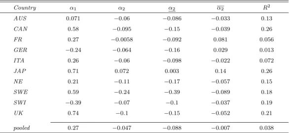
Test of the Correlation Mechanism In addition, we document some direct evidence in the data for the correlation mechanism. For data reasons, we focus on non-durable consumption growth only. Using a sample of ten developed countries, we regressed a country’s non-durable consumption growth on US non-durable consumption growth and US consumption growth interacted with the lagged interest rate differential:

∆ci_t+1 =α0+α1∆cU St+1+α2

Ri,_t£−R$_t∆cU S_t+1+ǫt+1.

The results obtained over the post-Bretton Woods period on annual data are reported in table 9. The coefficients on the interaction terms α2 are negative for all countries, except

for Japan. The table also reports ninety percent confidence intervals for these interaction coefficients. They show that the α2 coefficients are significantly negative for 7 countries. The

last row of each panel reports the pooled time series regression results. The ninety percent confidence interval includes only negative coefficients.

As is clear from the α2 estimates in column 3, the conditional correlation between foreign

and US annual consumption growth decreases with the interest rate gap for all countries except Japan. We also found the same pattern for Japanese and UK consumption growth processes (not reported).

V

Robustness

This section goes through a number of robustness checks: (1) we look at other factor models, (2) we split up the sample, (3) we introduce other test assets, (4) we re-estimate the model on developed currency portfolios, and (5) we re-estimate the model using the Generalized Method of Moments.