UNIVERSITY OF READING
Department of Meteorology
On the Behaviour of Tropical
Depressions and their Interaction
with the Indian Monsoon Trough
Region
Kieran Mark Rainwater Hunt
A thesis submitted for the degree of Doctor of Philosophy
December 2016
DECLARATION
I confirm that this is my own work and the use of all material from other sources has been properly and fully acknowledged.
This thesis examines the behaviour of Indian monsoon depressions (MDs), synoptic-scale systems that frequent the monsoon trough throughout the boreal summer. The original contribution to knowledge is a substantial advancement of our understanding on the structure, variability, and dynamics of MDs. A feature-tracking algorithm is developed to emulate the subjective methods used by the India Meteorological Depart-ment, based on surface wind speed and surface pressure. This is applied to reanalysis data spanning from 1979 to the present day (2016), extracting 106 events. These are used to build a statistical composite, with which we interrogate the structure and vari-ability subject to external forcings. It is found, for example, that MDs significantly
intensify during La Ni˜na and active monsoon spells, and have different spatial structure
over ocean than land. These events are also examined in satellite data, where we dis-cover and characterise a bimodal, diurnal cycle in surface precipitation; the structure of cloud type with dominating deep convection south of the centre; and present the first composite picture of vertical hydrometeor structure in MDs. A propagation mecha-nism whereby the MD behaves as a vortex in the presence of a wall (i.e. the Himalayan massif) is presented and shown to perform better than competing theories at predicting the velocity and heading of MDs. It is also shown, using a case study in the Met Office Unified Model (MetUM), that varying antecedent soil moisture conditions can signifi-cantly change the length of a MD track but not its direction. The sensitivity of MDs to changes in horizontal resolution in the MetUM are also explored across seven case studies at eight resolutions. It is found that the intensity is typically slightly overpre-dicted, correlating with too great a latent heat release in the mid-troposphere. Spatial structure is shown to improve with resolution but improvement saturates beyond N512 (40 km) resolution.
ACKNOWLEDGEMENTS
I thank my supervisors, Andy Turner, Pete Inness, David Parker, and Richard Levine for their invaluable guidance and constructive criticism of this work in its entirety. I
would especially like to thank Andy, who often went above and beyond the rˆole of
supervisor in his friendly and generous encouragement, both academic and pastoral. I
would also like to thank Gill Martin for her support during my involvement with the Met Office, and Steve Woolnough and Emily Black for their rigorous, biannual quality control.
List of Figures . . . vii
List of Tables . . . xix
1 Introduction 1 1.1 Background . . . 1
1.2 Motivation . . . 6
2 Data and Methods 11 2.1 Tracking algorithm . . . 11
2.1.1 Motivation . . . 11
2.1.2 Counting contours . . . 13
2.1.3 Wind criteria . . . 17
2.1.4 Vorticity filters . . . 18
2.1.5 Linking candidates to form a track . . . 19
2.1.6 Recent developments to the tracking algorithm . . . 21
2.2 Data overview . . . 22
2.2.1 ERA-Interim reanalysis . . . 22
2.2.2 Tropical Rainfall Measuring Mission . . . 24
2.2.3 CloudSat . . . 25
3 On the structure and dynamics of Indian monsoon depressions 26 3.1 Introduction . . . 26
3.2 Methodology . . . 28
3.2.1 Data . . . 28
3.2.2 Tracking software . . . 29
3.2.4 Choosing a suitable climatology . . . 31
3.3 Composite horizontal structure . . . 31
3.3.1 Precipitation . . . 31
3.3.2 Reanalysis fields . . . 33
3.4 Composite vertical structure . . . 38
3.4.1 Moisture . . . 38
3.4.2 Cloud features . . . 39
3.4.3 Potential vorticity and circulation . . . 40
3.4.4 Moisture flux . . . 43
3.4.5 Temperature profile . . . 44
3.4.6 CAPE and tephigram analysis . . . 47
3.4.7 Summary of composite vertical structure . . . 52
3.5 Variability within the composite . . . 52
3.5.1 Variability over the lifetime . . . 52
3.5.2 Coastal transitions and the land-sea contrast . . . 54
3.5.3 Diurnal cycle . . . 58
3.6 The influence of large-scale forcing . . . 59
3.6.1 El Ni˜no Southern Oscillation . . . 61
3.6.2 The Indian Ocean Dipole . . . 63
3.6.3 Active and break phases . . . 65
3.7 Conclusion and discussion . . . 67
4 The spatiotemporal structure of precipitation in Indian monsoon depressions 70 4.1 Introduction . . . 70 4.2 Methodology . . . 72 4.2.1 Data . . . 72 4.2.2 Compositing . . . 74 4.3 Composite structure . . . 75 4.3.1 Hydrometeor distributions . . . 75 4.3.2 Cloud scenario . . . 79
4.3.3 Diabatic heating: latent and radiative . . . 85
4.3.4 Reanalysis composite . . . 87
4.4 Case study . . . 89
4.5 Diurnal variability . . . 98
5 The movement of Indian monsoon depressions by interaction with image
vortices near the Himalayan Wall 104
5.1 Introduction . . . 104
5.2 Data and methods . . . 110
5.3 Results . . . 112
5.4 Conclusions . . . 115
6 The effect of horizontal resolution on Indian monsoon depressions in the Met Office NWP model 118 6.1 Introduction . . . 118
6.2 The Met Office Unified Model and experimental setup . . . 119
6.2.1 Case study selection . . . 120
6.2.2 Overview of the Unified Model . . . 120
6.2.3 The spectrum of resolutions . . . 123
6.2.4 Description of the tracking algorithm . . . 123
6.2.5 Adaptive downsampling . . . 124
6.3 Propagation and duration . . . 126
6.4 Representation of the monsoon trough during depressions . . . 127
6.4.1 Rainfall . . . 129
6.4.2 Synoptic circulation . . . 131
6.5 Evaluation of composite depression structure . . . 133
6.5.1 Vertical structure . . . 136
6.5.2 Horizontal structure . . . 141
6.5.3 Cloud structure . . . 144
6.5.4 Diurnal cycle . . . 146
6.6 Conclusions . . . 150
7 The effect of soil moisture perturbations on Indian monsoon depressions in a numerical weather prediction model 153 7.1 Introduction . . . 153
7.2 The Met Office Unified Model and experimental setup . . . 158
7.2.1 Overview and case study selection . . . 158
7.2.2 The land surface scheme . . . 158
7.2.3 Ensemble generation . . . 159
7.2.4 Soil moisture ancillaries . . . 160
7.2.5 Tracking . . . 161
7.3 Results . . . 162
7.3.2 Structure and evolution . . . 164
7.4 Discussion and conclusion . . . 170
8 Conclusions and future work 173 8.1 Discussion . . . 173
8.2 Limitations . . . 175
8.3 Future work . . . 177
8.4 Applications and implications . . . 181
A Formal description of system composite 183
B Derivation of cylindrical model propagation velocity 185 C Overview of the land surface scheme used in the model 188
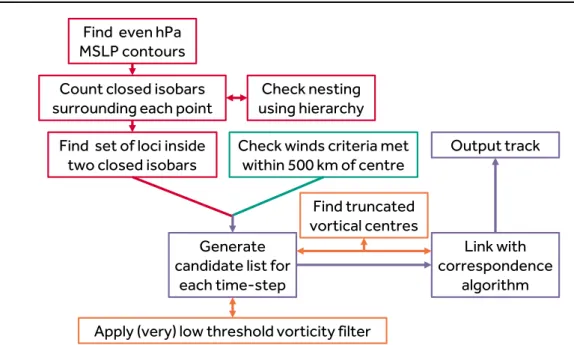
2.1 Schematic of the tracking algorithm. Descriptions of each term are given in the text. Red, turquoise, orange, and purple boxes are described in
§2.1.2, §2.1.3, §2.1.4 and §2.1.5 respectively. . . 12
2.2 Simple example of the interpolating contour-seeking algorithm discussed
in the text. The values of the bivariate field are defined at each grid vertex, and the points of intersection of the contour lines are determined by interpolation. Here, the red line represents part of a contour set of
value 5, and the cyan line is of value 6. . . 14
2.3 Example contour polygon subtree including MD signal; this is for mean
sea-level pressure (even hPa intervals) at 2014-08-04 06Z. Dotted red lines indicate the links between selected contour polygons on the map and tree, orange ellipses denote possible MD candidates according to the two closed contour requirement, green crosses indicate that the contour polygon would be rejected for intersecting the domain boundary, and blue crosses indicate that the contour polygon would be rejected for
having more than one child. . . 16
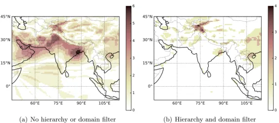
2.4 The results of the contour counting algorithm for ERA-Interim
reanal-ysis mean sea-level pressure at 2014-08-04 06Z, (a) without applying the additional stability filters discussed in the text, and (b) with them. Colour indicates contour count as described by the respective colour bars. 17
2.5 Simple application of our correspondence algorithm. Left: red markers indicate identified candidates according to wind speed/surface pressure criteria, with numbers representing some arbitrary timestamp. Centre: existing candidates are attached to the nearest vorticity local maximum (orange markers), and phantom points are interpolated for timestamps with missing candidates (white markers). Right: phantom points are
attached to nearest vorticity local maximum and the track is completed. 21
3.1 Depression tracks from (a) the 106 depressions used in this study, and (b)
the 98 depressions from the dataset outlined by Hurley and Boos (2015) that fulfil our location criteria. Note that Hurley and Boos (2015) also defined their tracks under monsoon low conditions. Colour indicates
depression intensity using SLP anomaly to a 21-day running mean. . . . 28
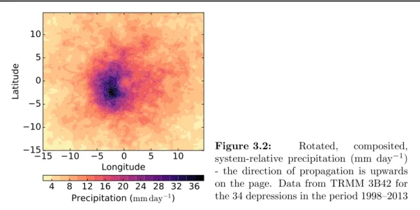
3.2 Rotated, composited, system-relative precipitation (mm day−1) - the
direction of propagation is upwards on the page. Data from TRMM
3B42 for the 34 depressions in the period 1998–2013 . . . 32
3.3 Composite precipitation data from TRMM 3B42 for the 34 depressions
in the period 1998–2013. (a) average precipitation (mm day−1) for South
Asia on depression days; and (b) the difference between depression days
and the boreal summer mean (colours), and their ratio (lines). . . 33
3.4 850 hPa wind speed (m s−1) in coloured contours, with wind vectors
overlaid, for the 106-depression composite, using ERA-Interim reanalysis data over 1979–2014, for (a) the full composite, and (b) the composite as an anomaly to the summer mean circulation. Coloured contours are greyed out where the composite does not significantly differ from the
climatology at the 95% level. . . 35
3.5 Composite relative vorticity (10−5s−1) shown as shading in the (a) lower
and (b) upper troposphere along with line contours indicating (a) surface pressure and (b) 200 hPa geopotential height. Positive vorticity indicates cyclonic, counterclockwise rotation. Line contours become blue dashes where the composite does not differ significantly from the climatology at the 95% level; likewise, coloured contours are reduced to 20% intensity. 36
3.6 2-m temperature anomalies (K) in coloured contours, 350 hPa
temper-ature anomalies (K) in line contours. Both shown as anomalies to the
3.7 Composite relative humidity (%) at 850 hPa in coloured contours with total cloud cover (%) in line contours. Statistical significance is displayed
as in Fig. 3.5. . . 36
3.8 Composite boundary layer height (m, coloured contours) and
bound-ary layer dissipation (W m−2, line contours). Statistical significance is
displayed as in Fig. 3.5. . . 37
3.9 Composite surface latent heat flux (W m−2, coloured contours) and
sur-face sensible heat flux (W m−2, line contours). Statistical significance is
displayed as in Fig. 3.5. . . 37
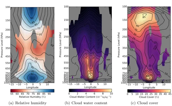
3.10 (a) relative humidity (%), (b) cloud water content (10−5 kg kg−1; the
summation of liquid and ice contributions), and (c) cloud cover (fraction of unity) as functions of pressure levels as viewed on a plane normal to the direction of depression propagation. Direction of propagation into the page. Coloured contours are greyed out where the composite does
not significantly differ from the climatology at the 95% level. . . 39
3.11 Following Fig. 3.10(a). Vertical structure of relative humidity (%) as an
anomaly to the summer climatology. . . 40
3.12 View and significance as defined in Fig 3.10, (a) potential vorticity
(10−7 K m2 kg−1 s−1), (b) tangential wind speed (m s−1 - positive
val-ues going into the page, negative coming out), and (c) relative vorticity
(10−5 s−1), all viewed as anomalies to the summer climatology. Note
the different y-axis for (a). . . 41
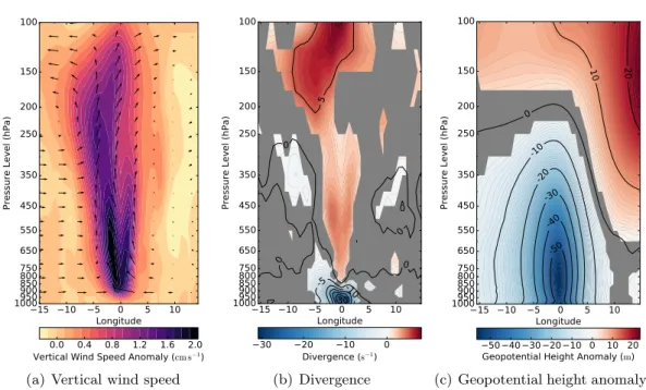
3.13 View and significance as defined in Fig 3.10. (a) vertical wind speed
(cm s−1) and quivers for vertical/zonal wind at the cross-section
bound-ary, the vertical component is increased by a factor of 100 for the quivers;
(b) divergence (10−6 s−1); (c) geopotential height (m) as an anomaly to
the summer climatology. . . 42
3.14 Vertical structure of the three specific humidity flux perturbation terms
from eq. 3.1 (kg kg−1m s−1) and associated convergence (kg kg−1s−1) in
coloured contours: (a) the anomalous moisture advected by the climato-logical wind, (b) the climatoclimato-logical moisture advected by the anomalous wind, and (c) the anomalous moisture advected by the anomalous wind. Colours are greyed where the moisture flux is not significantly different at the 95% confidence level from a bootstrapped zero-centred distribution derived from differencing random pairs of samples from the composite
of qv. Note the differing colour scales and unit vectors. Quivers are
3.15 Vertical structure of (a) temperature (K), (b) potential temperature anomaly (K), and (c) equivalent potential temperature anomaly (K). Colours are greyed out where the profiles are not significantly different
from the climatology at the 95% significance level. . . 45
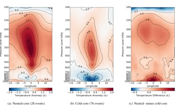
3.16 Vertical structure of the temperature (K) as an anomaly to the boreal summer mean for a composite depression with both main core cate-gories, and their difference: (a) neutral-core, (b) cold-core, (c) their difference. In (a) and (b), colours are greyed out where the subsets do not significantly differ from the full composite temperature profile at the 95% confidence level, ascertained by the bootstrapping method; in (c), colours are greyed out where the difference does not significantly differ from zero at the 95% confidence level using the bootstrapping difference
method on the full composite temperature profile. . . 46
3.17 Horizontal composite of CAPE (J kg−1) in coloured contours and CIN
(J kg−1) in line contours. Significance as in Fig. 3.5 . . . 48
3.18 Tephigrams of simulated soundings going through the centre of the com-posite depression and selected subsets. Temperature in red, dew point
temperature in blue. . . 49
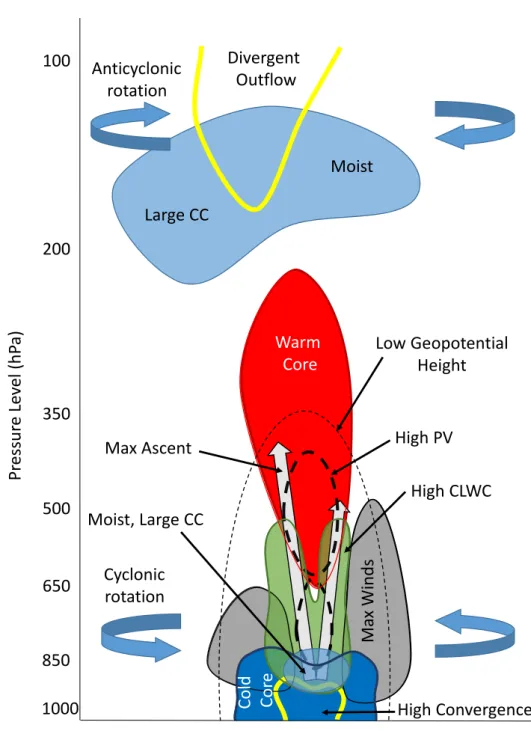
3.19 Schematic of the composite monsoon depression. CC = cloud cover;
CLWC = cloud liquid water content; PV = potential vorticity. . . 51
3.20 (a) Surface pressure anomaly at centre (hPa), maximum 850 hPa wind
speed anomaly (m s−1), and 850 hPa central relative vorticity anomaly
(10−5s−1) of the composite depression as a function of percentage of
life-time duration, with respective percentage of systems over land, coast (de-fined as within 150 km of coastline) and sea shown underneath, anomalies are relative to a 21-day running mean; and (b) histogram of depression durations, with the generalised logistic function fitted. The mean
de-pression duration is 3.3 days, with a standard deviation of 1.6 days. . . 53
3.21 Vertical structure of equivalent potential temperature (K) ocean, coastal, and land composites. Colours are greyed out where the subset is not significantly different from the full composite at the 95% confidence level. 55
3.22 Vertical structure of wind speed anomaly (m s−1) for purely oceanic
and land-based composite depressions; (c) shows their difference.
Sig-nificance as in Fig. 3.16 . . . 56
3.23 Vertical structure of the ocean-minus-land composite (as in Fig. 3.22(c))
for specific humidity (10−4 kg kg−1), relative vorticity (10−5 s−1), and
3.24 Diurnal variation as represented by a day-minus-night composite for (a) temperature (K), (b) relative humidity (%), and (c) cloud cover (%).
Significance as in Fig. 3.16(c) . . . 58
3.25 TRMM rainfall difference composites (mm day−1) for (a) El Ni˜no minus
La Ni˜na and (b) active-minus-normal. . . 59
3.26 Vertical structure of the (a-c) El-Ni˜no-minus-La-Ni˜na, (d-f) IOD
positive-minus-negative and (g-i) active-minus-neutral composites for (a,d,g) geopo-tential height (m), (b,e,h) temperature (K) and (c,f,i) specific humidity
(10−4 kg kg−1) respectively. The colours are greyed out in areas where
the composite difference does not significantly differ from zero. . . 60
3.27 Surface temperature (K, coloured contours) and wind (m s−1) at 850 hPa
for (a) IOD positive-minus-negative and (b) El Ni˜no-minus-La Ni˜na
de-pression days. Note the differing colour scales. . . 64
3.28 Relative vorticity (coloured contours, 10−5s−1) and wind (m s−1) for (a)
all depression days as an anomaly to the boreal summer mean and (b) active-minus-neutral depression days. The coloured contours are greyed
out where the orography rises above the 850 hPa level. . . 66
4.1 Composite mean surface precipitation (mm day−1) from TRMM 3B42
for depressions 1997-2014. Right: the rotated composite, where each timestep is rotated such that the depression is heading due north (i.e. up
the page). Left: as right, but with no rotation during compositing. . . . 76
4.2 Composite vertical profile of rain rate (mm day−1, coloured contours)
from TRMM 2A25 as a function of pseudoradius. Overlaid as a dark grey line for illustration is the (unrotated) composite surface rain rate
(mm day−1, right axis) from TRMM 3B42 (see Fig. 4.1(a)), also as a
function of pseudoradius. Note that the lowest contour is coloured white,
and the background, grey. . . 77
4.3 Modal raindrop size (mm, radius) throughout the composite, calculated
from the drop size distribution parameters in TRMM 2B31. Right: full distributions for selected pseudoradii at a height of 1.5 km, the locations
of which are indicated by dots on the left hand figure. . . 77
4.4 Composite vertical profile of graupel (g m−3, top) and snow (g m−3,
mid-dle) densities as a function of pseudoradius, from TRMM 2B31. Under-neath are the structures of the bright band, storm, and freezing heights, from TRMM 2A23. Note the height scales differ between the top two and bottom panels. The colour scale is the same for both relevant panels. 78
4.5 Modal cloud scenario in the composite, determined by CloudSat 2B-CLDCLASS. Differing hues represent varying cloud types, with the trans-parency in each case proportional to the ratio of the modal value and the number of overpasses up to a value of 0.5. Parts of the composite not comprising at least ten satellite overpasses are not shown here. We remind the reader that CloudSat height is referenced above the geoid
rather than necessarily the Earth’s surface. . . 80
4.6 Left: cloud cover (fraction of unity) as a function of pseudoradius, as
calculated from composite 2B-CLDCLASS data. Right: as left, using ERA-I data. For consistency, both are composited using the same
tech-nique. . . 82
4.7 Contoured frequency by altitude diagram (CFAD; Yuter and Houze,
1995) for effective radar reflectivity at 13.8 GHz (dBZ) from TRMM
2A25, at pseudoradii of -10◦ (left), -4◦ (centre), and 10◦ (right). The
abscissa starts at 15 dBZ, the approximate value of the TRMM PR
sensitivity threshold. . . 83
4.8 As Fig. 4.7 but for radar reflectivities at 94 GHz from CloudSat
2B-GEOPROF. Again, at pseudoradii of -10◦(left), -4◦(centre), and 10◦(right). 83
4.9 Composite rain fraction computed using objective rain type from TRMM
2A23 and estimated surface rain rate from TRMM 2A25. Left: convec-tive; centre: stratiform; right: events not attributable to the previous
two categories. See text for a definition of “definitely”. . . 84
4.10 As Fig. 4.9 but using a “maybe” threshold (i.e. up to and including
“definitely”). Left: convective; centre: stratiform; right: events not
attributable to the previous two categories. . . 84
4.11 Composite vertical radiative heating profile (K hr−1) within the MD
from both longwave and shortwave radiation, derived from CloudSat
2B-FLXHR. Data removed as per Fig. 4.5. . . 86
4.12 Left: composite vertical latent heating profile (K hr−1) from
hydrome-teor fluxes within the MD as a function of pseudoradius, derived from TRMM 2B31. Right: two selected vertical profiles from the
compos-ite, -5◦ (magenta) and -2◦ (green). Note the short vertical axis due to
negligible mean latent heating rate above the freezing level. . . 86
4.13 Several composite variables as functions of pseudoradii and height. Left: temperature (K) as an anomaly to the boreal summer mean, centre:
vertical velocity (m s−1, positive upwards), right: divergence (10−6s−1).
4.14 Path of the early July 2007 MD: 6 hourly intervals plotted in cyan mark-ers, with the location at 0000UTC 07 July in yellow. The areas cov-ered by the TRMM and CloudSat overpasses are bounded by red and green lines respectively. The locations of the 16 rain gauges used in the rainfall comparison are also shown, west to east they are: Jaipur (Ja), Guna (Gu), Bhopal (Bh), Gwalior (Gw), Jabalpur (Jb), Satna (S), Pen-dra Road (P), Jharsuguda (Jh), Gaya (Ga), Ranchi (R), Balasore (Bl), Kolkata (K), Ishwardi (I), Jessore (Je), Barisal (Br), and Chittagong (C). Overlaid (coloured contours, mm) is the total precipitation for the
UTC day 07 July. . . 90
4.15 Selected data from the TRMM and CloudSat overpasses designated in Fig. 4.14; the bottom two panels are 12Z ERA-Interim data taken as close as possible to the CloudSat overpass path. ‘C’ on each abscissa marks the location of the centre of the depression at the time of the overpass. Where ERA-I data would be subterranean, they are greyed out. 94 4.16 Tephigrams for soundings from three consecutive days at Ranchi station
(see Fig. 4.14). Red and blue lines show temperature (K) and dewpoint (K) profiles respectively, and on the right of each tephigram, the wind
barbs (m s−1) are shown in black. Where ERA-Interim data would be
below the surface, they are greyed out. . . 96
4.17 Comparison of the average daily precipitation (mm day−1) recorded at
the sixteen stations shown in Fig. 4.14 during the depression of early July 2007. Gauge values are given in green, TRMM 3B42 estimates are
given in blue. Each shown with a 1σ band. Where gauge measurements
were missing, TRMM data were also omitted from the average. . . 97
4.18 Daily precipitation (mm day−1) for eight selected stations along the path
of the depression in early July 2007, approximately from east to west. Gauge values are given in green, TRMM 3B42 estimates are given in blue. 97
4.19 Composite rotated structure of surface precipitation rate (mm day−1)
in MDs at three hour intervals across the UTC day as anomaly to the
mean, derived from TRMM 3B42. . . 99
4.20 Amplitudes of the two diurnal modes of surface precipitation (mm day−1)
in the rotated composite, derived from TRMM 3B42. . . 101
5.1 Mean boreal summer (JJAS) 850 hPa wind vectors with MD tracks
5.2 Flow around a pair of counter-rotating ideal point vortices, identical to an ideal point vortex, V, and its corresponding image vortex, I, in the image plane (grey). . . 107
5.3 Composite 850 hPa MD winds with the boreal summer climatology
sub-tracted (as Fig. 3.4(b)). In this composite, the data for individual time steps are rotated such that the direction of propagation is due north (up
the page) and translated such that the centre is at 0◦N, 0◦W on a regular
lat/lon grid. Here, therefore, the Himalayas lie to the right. . . 108
5.4 Modified from Fig. 3.28, 850 hPa relative vorticity (10−5 s−1) on
June-September depression days as an anomaly to the boreal summer mean; greyed out where the orography is higher than the 850 hPa level. The green line represents the average path of tracked depressions. . . 109
5.5 Histogram showing the ratio of observed to predicted IMD propagation
velocities for each of the five models discussed in the text calculated for all timesteps present in the dataset. Red and blue represent our lin-ear and cylindrical models respectively; black represents a simple model based on the climatology; dashed green (magenta) represents a simple beta drift model (not) including background monsoonal flow. . . 113
5.6 As with Fig. 5.5 but showing the difference between the predicted
head-ing and the observed headhead-ing. . . 113
6.1 Comparison of official IMD tracks (solid) with those tracked objectively
from ERA-Interim (dashed). The average length of the latter is longer due to the relaxed MD wind criterion used in this study. Depression start dates are as given in Table 6.1. . . 121
6.2 Pictorial example of adaptive downscaling from an 8×8 grid to a 3×3
grid. The leftmost grid (8×8) contains some sparse data, represented
by the orange and blue blocks; firstly the resolution is reduced to the
closest divisor of the original that is higher than the target (here 4×4,
as 4|8 and 4≥3). We then use a two-dimensional interpolation method
to downsample from this intermediate resolution to the final 3×3 grid. 125
6.3 A selection of tracks from the case study experiments. In bold are the
mean tracks for each resolution, normalised by duration; the westward propagating tracks that traverse the peninsula are from the 16/09/2015 MD, and those propagating northwards toward the Ganges Delta are from the 20/06/2015 MD. In black are the tracks computed from ERA-Interim, and in grey are the official IMD tracks. . . 126
6.4 Mean distance from (a) ERA-Interim track and (b) IMD track as a function MD lifetime percentage. Duration normalisation is carried out before averaging, as in Fig. 6.3. . . 127
6.5 Mean precipitation (mm day−1) in the monsoon depression-trough and
surrounding area for a selection of resolutions, compared against the same period(s) for TRMM-TMPA 3B42. Each is averaged over the same set of dates and times: those in which a MD was considered present in ERA-Interim by our tracking algorithm. . . 128
6.6 Fraction of total time for which “very heavy” rainfall events were present
in the depression-trough for a selection of resolutions, compared against the same period(s) for TRMM-TMPA 3B42. “Very heavy” is defined by
the IMD as rates exceeding 125 mm day−1. Computation as in Fig. 6.5. 128
6.7 Normalised log-histogram of precipitation (mm day−1) in the
depression-trough during the case-study MDs. Here, the depression-trough is defined simply
as a box bound by the coordinates: 20-25◦N, 75-85◦E. Breaks in lines
indicate zero counts. . . 129
6.8 Mean 500 hPa relative humidity and 500 hPa winds in the monsoon
depression-trough and surrounding area for a selection of resolutions, compared against the same period(s) for ERA-Interim. Computation as
in Fig. 6.5. . . 131
6.9 Mean 700 hPa potential vorticity (10−7K m2kg−1s−1) and 850 hPa
winds in the monsoon depression-trough and surrounding area for a selection of resolutions, compared against the same period(s) for ERA-Interim. Computation as in Fig. 6.5. Where orography is above 700 hPa, the coloured contours are greyed out. . . 132
6.10 A selection of intensity diagnostics as functions of resolution. From
top to bottom: minimum surface pressure obtained (hPa), maximum temperature anomaly at 350 hPa relative to climatology (K), mean pre-cipitable water (mm), and maximum free convective depth (km). Each is computed from a 1000 km-sided box surrounding the centre, with the value for each MD case study; these individual values are plotted as blue circles at each resolution with the mean given by the blue line. The green line represents the value obtained by performing the same compu-tation on the ERA-I track. Here, free convective depth is defined as the difference in altitude between the levels of free convection and neutral buoyancy. . . 134
6.11 Mean composite potential vorticity (10−7K m2kg−1s−1) for the case study MDs. Tracked MDs in the forecasts and reanalysis are centralised such that their centres lie at the origin of the composite. Here, south-north cross-sections through the composite origin are presented for all resolutions, and the composites derived from both our ERA-I tracks and the IMD tracks (i.e. the tracks determined from ERA-I and those given by the IMD, both applied to ERA-I data – see text for more details).
The reader is reminded that the ERA-I equatorial resolution of∼78 km
is approximately N256 (in reality, it is exactly T255). . . 137
6.12 Normalised histograms of relative vorticity (10−5s−1) for each resolution
and the ERA-I and IMD tracks. These are taken at all times where an MD is present, from a cuboid of horizontal length 400 km centred on the origin, and vertical extent (a) 925-750 hPa and (b) 650-300 hPa. . . 138 6.13 Mean composite temperature anomaly (K) for the case study MDs.
Compositing method as in Fig. 6.11. Here the anomaly is against the climatology computed for the thirty-seven total forecast days (with these dates also used to compute climatology for the reanalysis structures). . . 139
6.14 Mean composite wind speed anomaly (m s−1) for the case study MDs.
Construction of the composite is as Fig. 6.11 and the anomaly is taken against the climatology, whose computation is as in Fig. 6.13. . . 139
6.15 Composite total surface precipitation (mm day−1, method as in Fig. 6.11)
for all resolutions, as well as for the ERA-I and IMD case study tracks as computed from TRMM 3B42. . . 142
6.16 Composite CAPE (J kg−1, filled contours) and total column precipitable
water (mm, line contours) for each resolution, as well as for the ERA-I and IMD case study tracks as computed from ERA-Interim. . . 143 6.17 Composite cloud cover fraction for all resolutions, and ERA-I and IMD
tracks determined from ERA-I. The bounding heights for the model cloud levels are defined on sigma levels that from the surface equate
to 0.0 km≤low<1.8 km≤mid<5.5 km≤high<13.7 km, and for
ERA-I reanalysis are defined on sigma levels that from the surface equate
to 0.0 km≤low<1.9 km≤mid<6.3 km≤high. The colour scheme is
ex-plained in the right-hand subfigure. . . 144 6.18 Amplitude, as a function of time (UTC) of the central (c-) mode for
precipitation (mm hr−1) for MDs across all resolutions (solid, coloured),
and the climatology for ERA-I-tracked MDs in TRMM 3B42 (dashed, black). . . 148
6.19 Composite fraction of surface precipitation caused by stratiform pro-cesses (as opposed to convective) in the model, across all resolutions. This is intended to allow direct comparison with the values from TRMM
climatologies in Figs. 4.9 and 4.10 . . . 148
7.1 Bowen ratio (lines) and precipitation (colours) for a 34-depression
com-posite (1998-2014), as described in §3.3.1; the composite is normalised
such that the centre of each depression is placed at the origin, and each is rotated so that the heading is up the page. For both fields, only points
over land were composited. . . 155
7.2 Monthly soil moisture climatologies for the Indian peninsula from two
products: (a) NOAA CPC reanalysis total soil moisture (data pro-vided by the NOAA/OAR/ESRL PSD, Boulder, Colorado, USA, from
their website at http://www.esrl.noaa.gov/psd/) and (b) ESA CCI
satellite-derived volumetric soil moisture. . . 156
7.3 Average MD tracks for each month (June through September
repre-sented by red, blue, green, and black respectively) during the Indian monsoon. Solid lines represent mean tracks from the database outlined
in §3, dashed lines from the Hurley and Boos (2015) database. These
tracks also include days where the disturbance is classified as a monsoon low, as well as a monsoon depression. . . 156
7.4 Map showing the three masks used in the experiments in this study.
The red box covers the entire peninsula and some of the rest of South Asia, the green box approximates the region where the monsoon trough is most active, and the orange box covers the intensely irrigated and
farmed area in the Himalayan foothills. . . 160
7.5 Track results from varying soil moisture in (a) the monsoon trough and
(b) the sub-Himalayanarable zone. For each sub-experiment, the average
track is given by the thick line with its termination given by the filled circles, and the individual ensemble 10-member track terminations are given by crosses of the same colour. Also shown, in pale green, is a concave hull of the “100%” (for (a), this is simply the control) ensemble plume for each experiment. In (a), the official MD track from the Indian Meteorology Department is given by the solid black line; in (b), the
7.6 Differences in selected fields of the composite mean ensembles for the
500% and 1% (the former minus the latter) trough zone experiment.
The composite is normalised such that its centre lies at the origin, but no rotation is carried out; these are then presented as a height-longitude cross section (at zero latitude). Greyed areas indicate the difference between the sub-experiment composites was not met at the 95% signif-icance level according to a 10,000 member bootstrap test. The selected
fields are: (a) potential vorticity (10−7 K m2 kg−1 s−1), (b) relative
humidity (%), and (c) temperature (K). White lines on each subfigure indicate the zero contour. . . 165
7.7 Longitude-latitude cross-sections of composite precipitation (mm day−1)
and 850 hPa winds, taken as the difference of the ensemble means for the 500% and 1% sub-experiments (i.e. 500% mean minus 1% mean)
of (a) the trough zone experiment and (b) the arable zone experiment.
Construction and representation of significance are identical to that of Fig. 7.6. Note that while these composites are centred on the MD, they are not rotated. . . 166
7.8 Differences in selected fields of the composite mean ensembles for the
500% and 1%arable zone experiment. Construction identical to Fig. 7.6,
except that these are latitude-height cross-sections. The selected fields
are: (a) potential vorticity (10−7 K m2 kg−1 s−1), (b) relative humidity
(%), and (c) temperature (K). White lines on each subfigure indicate the zero contour. . . 167
7.9 Selected fields as a function of normalised depression lifetime for the
trough experiment, with the soil moisture changes coloured thus: 1% -red, 80% - yellow, 120% - green, 500% - blue.
From top to bottom, they are: the maximum CAPE (J kg−1) found in
the advance quadrant1of the MD; mean total precipitable water (mm);
mean temperature anomaly (K) between 850 and 400 hPa; and
maxi-mum relative vorticity (10−5s−1). Each is computed over a box of side
length 250 km centred on the MD centre.
The thick, solid lines represent the ensemble average, with the thinner,
1.1 A summary of the published/submitted papers that comprise this thesis,
ordered by submission date. . . 2
1.2 The most recent official classifications for monsoon disturbances, as
out-lined by the glossary published by the India Meteorological Department (e.g. IMD, 2015). Ω is the count of closed even isobars (i.e. ..., 998, 1000,
1002, ... hPa) at the surface, U∗ is the surface wind speed. All relevant
criteria must be met for the classification to be made. 1 knot = 0.51 m s−1. 3
1.3 Summary, by month of genesis, of cyclonic events in India and
surround-ing seas (the Bay of Bengal and the Arabian Sea) from 1891-2014. Events are classified by the maximum intensity reached during their lifetime (D = depression or deep depression, CS = cyclonic storm, SCS = severe, very severe, or super cyclonic storm), and the bracketed values are for events whose geneses were in the Bay of Bengal. Data are from the IMD
eAtlas. . . 4
3.1 Some data showing rainfall rates (mm day−1) of selected percentiles for
cold- and neutral-core depressions over the domain used in, e.g. Fig. 3.17. 47
3.2 Some tephigram data for different composites. Abbreviations: LCL
-lifted condensation level, LFC - level of free convection, LNB - level of neutral buoyancy, CAPE - convectively available potential energy, CIN - convective inhibition. These values were calculated directly from the
3.3 Distribution of depression days with respect to ENSO and active-break cycles. Active/break data are limited to July and August, and runs until 2010, so those events falling outside this period are tallied in the
penultimate column. . . 61
4.1 An overview of the TRMM algorithms and datasets used in this study. . 73
4.2 An overview of the CloudSat datasets used in this study. . . 74
5.1 Means and standard deviations of the normalised predicted velocity,|v−
vflow|/vmodel, and the error in predicted heading, θactual −θmodel, for
each of the five models. (Lin. = Linear, Cyl. = Cylindrical, Clim. = Climatology, B.D. = Beta Drift, B.D.F. = Beta Drift + Flow) . . . 115
6.1 A summary of the seven MDs used in this study. Data are computed
di-rectly from the high resolution IMD eAtlas tracks. Duration is defined as the total (contiguous) time for which the IMD classified the disturbance as a depression. . . 121
6.2 A summary of the eight horizontal resolutions used in this study, with
dimensions of the global grid, and zonal resolution at the equator. nx
andny refer to the number of longitudes and latitudes respectively used
to construct the grid. . . 124
6.3 Values (mm hr−1) and times (UTC) of the maxima and minima for the
outer (o-) and central (c-) modes of MD precipitation diurnal variability
(i.e. Aouter and Acentral respectively), computed from fitting eq. 4.5 to
the respective composites for each resolution. Also provided are the climatological values for MDs between 1998 and 2014 using TRMM 3B42
CHAPTER
1
INTRODUCTION
Opening remarks
This thesis is presented as a collection of five papers completed during the course of the degree, a summary of which is given in Tab. 1.1. Care has been taken to establish a good balance between literary unity of the thesis as a whole and keeping the individual chapters as faithful as possible to the form in which they were published/submitted. The fundamental differences lie in the introduction and conclusion sections of each chapter, which have been altered so as to lead into each other and shortened so as to reduce repetition.
1.1
Background
The South Asian monsoon (from Arabicmawsim, meaningseason) is a major
compo-nent in the global hydrological cycle, responsible for about 10000 km3 of rainfall per
season, or, approximately 10% of the annual global precipitation over land. This im-portant phenomenon is understood to come about through a reversal of the equatorial winds due to the heat low associated with the Indian peninsula, with blocking from the
Title Journal Submission Acceptance Citation On the structure and
dynam-ics of Indian Monsoon Depres-sions
Mon. Wea. Rev. 2014-11-13 2016-01-21 Hunt et al. (2016a)
The movement of Indian Mon-soon Depressions by interac-tion with image vortices near the Himalayan Wall
QJRMS 2015-01-20 2016-04-03 Hunt and Parker (2016)
The spatiotemporal structure
of precipitation in Indian
Monsoon Depressions
QJRMS 2016-01-08 2016-08-15 Hunt et al. (2016b)
The effect of soil moisture perturbations on Indian Mon-soon Depressions in a numer-ical weather prediction model
J. Clim. 2016-10-10 Hunt and Turner (2016)
The representation of Indian monsoon depressions at differ-ent horizontal resolutions in the Met Office Unified Model
QJRMS 2016-11-15 2017-03-03 Hunt and Turner (2017)
Table 1.1: A summary of the published/submitted papers that comprise this thesis, ordered
by submission date.
steep Himalayan orography, deep tropospheric temperature gradient from the elevated heating of the Tibetan Plateau, and in part, blocking from the Somali highlands. This moisture-laden westerly flow encircles the monsoon trough providing ample water for organised tropical convection over much of peninsular south Asia.
Embedded in the monsoon exist regular cyclonic disturbances that range in intensity from open easterly waves to full-blown tropical cyclones; such disturbances typically originate in the Bay of Bengal, or arrive there having passed over the Indochina penin-sula after genesis somewhere in the West Pacific. Either way, the Bay of Bengal provides almost ideal conditions to create or amplify these disturbances (Sikka, 1977): there are
warm SSTs (often in excess of 30◦C), the steeply curved eastern end of the cyclonic
monsoon trough is rich in lower-tropospheric vorticity, and there is the southern extent of the Tibetan anticyclone aloft that enhances divergent outflow. Monsoon
distur-Name General Ocean Land
Low Ω = 1 U∗ <17 kn Ω = 1 within 3◦
Depression Ω = 2,3 17 kn< U∗<27 kn Ω = 2 within 3◦
Deep depression Ω = 2,3 28 kn< U∗<33 kn Ω = 3,4 within 3◦
Cyclonic storm Ω>4 and 34 kn< U∗ <47 kn
Severe cyclonic storm Ω>4 and 48 kn< U∗ <63 kn
Very severe cyclonic storm Ω>4 and 63 kn< U∗ <119 kn
Super cyclonic storm Ω>4 andU∗>120 kn
Table 1.2: The most recent official classifications for monsoon disturbances, as outlined by the
glossary published by the India Meteorological Department (e.g. IMD, 2015). Ω is the count
of closed even isobars (i.e. ..., 998, 1000, 1002, ... hPa) at the surface,U∗ is the surface wind
speed. All relevant criteria must be met for the classification to be made. 1 knot = 0.51 m s−1.
bances are classified by the India Meteorological Department (IMD, 2015) into distinct categories based on surface wind speed and pressure anomalies, and these are collated in Tab. 1.2. For the sake of the rest of this work, ‘deep’ depressions will be merged with depressions to form a single category, as has been done by other authors (Cohen and Boos, 2014) and the IMD itself. The definitions given here are the most recent pub-lished by the IMD, and offer only slight variation from previous iterations (the general,
as opposed to land only, isobar criterion and the 3◦ constraint are not mentioned in
previous literature). It is rare to see a disturbance of cyclonic storm intensity or above during the monsoon season as the prominent westerlies in the lower troposphere and the tropical easterly jet in the upper troposphere result in substantial vertical wind shear that inhibits cyclonic development (Riehl and Shafer, 1944; DeMaria, 1996). To illustrate this, a summary of depressions, cyclonic storms, and severe cyclonic storms,
taken from the IMD eAtlas (http://www.rmcchennaieatlas.tn.nic.in/), is given in
Tab. 1.3. As can be seen from the table, depressions are by far most common during the months of the boreal summer (June - September), whereas the more intense storms peak outside the season in May, October, and November. A quick calculation from the data in Tab. 1.3 suggests a mean frequency of 4.8 MDs per season (June-September),
Month D(BoB) CS(BoB) SCS(BoB) January 11(11) 6(5) 2(2) February 4(4) 1(1) 1(1) March 2(2) 3(3) 2(2) April 10(7) 14(12) 18(14) May 38(29) 26(21) 60(41) June 107(72) 44(33) 20(5) July 144(104) 37(34) 8(8) August 188(151) 29(25) 3(3) September 160(124) 32(25) 20(15) October 122(100) 66(49) 53(41) November 65(44) 54(48) 86(70) December 39(32) 28(25) 27(25)
Table 1.3: Summary, by month of genesis, of cyclonic events in India and surrounding seas
(the Bay of Bengal and the Arabian Sea) from 1891-2014. Events are classified by the maximum intensity reached during their lifetime (D = depression or deep depression, CS = cyclonic storm, SCS = severe, very severe, or super cyclonic storm), and the bracketed values are for events whose geneses were in the Bay of Bengal. Data are from the IMD eAtlas.
an average of 3.6 of which spin up over the Bay of Bengal1, with a further 1.6 events
per season with a more intense classification than deep depressions.
With an average of 4-5 synoptic-scale disturbances moving across the peninsula each season, and an average duration of around 5 days (e.g. Yoon and Chen, 2005), we should expect these systems to be responsible for at least a significant minority of rainfall in the monsoon trough, where they are found most frequently Godbole (1977); Hurley and Boos (2015). Yet, there is huge variance on this number across previous studies: Dhar and Bhattacharya (1973) suggested a value around 10% over the Ganges basin; Mooley and Shukla (1989) found a value of 14% for the whole of India, and 27% for the central part; yet (Yoon and Chen, 2005) used a water budget analysis to determine the value was between 45% and 55%. This is surprising given the depth of careful work 1Many of the rest can be attributed to one of two sources: firstly, monsoon onset vortices in June
over the Arabian Sea (Krishnamurti et al., 1981) which have been known to develop into full-blown tropical cyclones (Willetts et al., 2016); and secondly, MDs can often spin up over land, typically in September, if the surface is wet enough (Hurley and Boos, 2015).
done on constraining precipitation in the context of individual monsoon depressions (e.g. Roy and Roy, 1930; Mull and Rao, 1949; Pisharoty and Asnani, 1957; Mooley, 1973; Rajamani and Rao, 1981; Kripalani and Singh, 1986), much of which draws on careful statistical analysis of rain gauge data. The difficulty in constraining this figure is made all the more troubling by Stowasser et al. (2009) who suggest that depressions will become more intense and precipitating in a warming climate. Despite issues with attribution of MD rainfall to monsoon totals, these studies have left us with a fairly sound picture of precipitation relative to the MD. We have known since Roy and Roy (1930) and Ramanathan and Ramakrishnan (1933) that MD precipitation is maximum southwest of the centre of the system; Pisharoty and Asnani (1957) produced the first significant analysis and suggested that rainfall in that area had an average maximum
of 75 mm day−1; Rajamani and Rao (1981) were the first to show that this asymmetry
was likely due to quasigeostrophic uplift, a fact forgotten until it was rediscovered independently by Boos et al. (2015). In addition, Mooley (1973) synthesised a number of synoptic hypotheses from previous literature that we will consider in further detail in Chapter 4.
The synoptic description of MDs led any serious dynamical treatment by several decades because upper air soundings were sufficiently rare to permit only intensive ob-servations of single events, compared to the general abundance of rain gauges. Many studies indeed analysed individual depressions (Das, 1952; Ananthakrishnan and Bha-tia, 1958; Koteswaram and George, 1958, 1960; Kulshrestha and Gupta, 1964; George and Datta, 1965; Rao and Rajamani, 1972; Daggupatty and Sikka, 1977; Rao et al., 1978) but it was not until the study of Godbole (1977) that the first three-dimensional picture emerged. He followed the examples of Reed and Recker (1971) and Williams and Gray (1973) for tropical wave disturbances in the Pacific and Frank (1977) for tropical cyclones and computed a five-depression composite for the disturbances of 1973, using approximately 100 upper air and 100 surface observations. Though lacking serious rigour and entirely lacking observations over the ocean (a common problem
until the satellite era), his study was the first to explicitly identify a number of features as being common to MDs: westward axial tilt with height, warm core aloft, circula-tion asymmetry, and dry mid-troposphere. Despite their use, and continued frequency for other types of disturbance, composite studies of MDs remained peculiarly sparse. Soon after, Keshavamurty et al. (1978) considered dynamic fields of a 15-depression composite, going so far as to subtract a climatology in an attempt to study MDs as the transient disturbances that they are. Later, Sarker and Choudhary (1988) looked at wind, moisture, and thermal fields of a 22-depression composite, and Prasad et al. (1990) looked at the wind and cloud structure of a 40-disturbance composite split by number of closed isobars; however neither study considered (and nor did Godbole, 1977, for example), the importance of removing monsoon westerlies to get a true picture, and so all came to the arguably incorrect conclusion that the strongest MD winds are found to the south of its centre.
More detailed background discussions are delegated to the chapters in which they are relevant.
1.2
Motivation
Given the frequency of these disturbances (Mooley and Shukla, 1989) and the quantity of rainfall associated with them (Pisharoty and Asnani, 1957), a sound understanding of their underlying structure and dynamics is crucial so that we can produce quality forecasts for the region (which depends heavily on its agrarian economy; Ramage, 1971; Jha, 2003). Further to this, understanding of MDs is also important for climate model simulations in light of poor representation of rainfall over the monsoon trough in many CMIP5 models and the climate configuration of the MetUM (Levine and Martin, 2016); improvement is crucial both for getting the climatology right and predicting future changes in extreme events. Despite this, attempts to interrogate the three-dimensional structure via a statistical treatment of observational data are approaching forty years
old and have a typically small sample size (Mulky and Banerji, 1960; Godbole, 1977; Sikka, 1977; Keshavamurty et al., 1978); those that are newer and have a larger sample size concern themselves with just a small handful of synoptic variables (Sarker and Choudhary, 1988; Prasad et al., 1990). In the modern era, where we have extensive reanalysis datasets assimilating globally reporting networks of automatic sensors and
dozens of satellites, no such study exists2, and we are left without a complete or reliable
database with which we can inform theory or models. What would such a composite structure look like? Would it be statistically robust? Using even an intermediate length
reanalysis, such as ERA-Interim (Dee et al., 2011, see§2.2.1 for details) which extends
from 1979 to the present would, at a conservative rate of two depressions per year give us a dataset of over eighty to analyse.
This presents an intermediate problem: with no tracking data available3, we must
generate our own if we are to produce any meaningful statistics. What then, is the best method for converting the subjective method used by the IMD for finding the trajectories of these systems into an objective, feature-based algorithm that can be applied to a suitable dataset? If this can be done successfully, we will have a sufficient sample size of MDs to be able to probe second-order questions about structure that will illuminate the relationship between these events and their environment, that is: how do monsoon depressions respond to large-scale forcing? This will open up questions about how ENSO, the Indian Ocean Dipole, and the active and break spells of the monsoon strengthen, weaken, or otherwise alter present MDs. This avenue can be expanded to consider smaller scales too: to what extent are depressions affected by a diurnal cycle? How do they behave over land as opposed to over the ocean? This latter question is of particular importance given the historical sparsity of ocean-based measurements. Now, assuming the sample size is sufficient, we should also be able to probe the structure
2
This was certainly true at the outset of this work, but has since been partially covered by the global depression climatology of Hurley and Boos (2015).
3
Except for those of the India Meteorological Department which are not made publicly available and those of Hurley and Boos (2015) which were not available at the commencement of this work (and use different criteria for the definition ofmonsoon depression).
with satellite data. This raises a new issue: given the data from satellite overpasses is not dense (cf. reanalysis), how can we construct a composite picture of MDs that has statistical significance? If we can solve this, we will be able to examine directly the vertical structure of important moist thermodynamical processes at a very fine resolution.
Quantifying the structure and variability of depressions is of clear importance, but it is static. If one wishes for a complete picture of these systems, we must also determine the process(es) governing their propagation. Climatologically, MDs that originate in or around the Bay of Bengal propagate northwestward (Sikka, 1977). This could probably be explained by beta drift if it were not for the fact that this underpredicts the propaga-tion speed and that depressions are embedded in strong lower-tropospheric westerlies. Historically, this anomalous movement has been attributed to quasigeostrophic vor-tex stretching towards the westsouthwest (Rao and Rajamani, 1970), the convergence maximum being southwest of the centre (Krishnamurti et al., 1975), or to anomalous circulation being supported by latent heat release above the precipitation maximum in the same place (Chen et al., 2005). Both of these hypotheses, however, predict south-westward, rather than northsouth-westward, propagation, and so are wrong by some ninety
degrees. To date, no study has addressed this issue4, and so we retain the question we
started with: what is the mechanism responsible for the northwestward propagation of monsoon depressions against monsoon westerlies? If such a singular dominant mech-anism (or coupled group thereof) does exist, it seems unlikely that it would not be further modulated by subordinate processes. For example, antecedent soil moisture in north India has been associated with extended MD duration (Chang et al., 2009), and assimilation of soil moisture data into numerical weather prediction models has been associated with improved track forecasts (Chandrasekar et al., 2008). So, how does the land surface state affect a passing depression?
At the start of this section, we part motivated this research into monsoon depres-4
Again, this was true at the outset of this work, but some advance has since been made by Boos et al. (2015).
sions by asserting that improved knowledge of their structure and behaviour would inform models and give us more material with which to validate their output. It is important, also, to determine how such systems are currently represented in models, a
problem which again lacks detailed analysis in existing literature5. This raises the first
important question: how well are depressions currently represented in global models?
This simple question opens the door to a salmagundi of others; of these, we shall
con-cern ourselves with those regarding how the representation can be improved. Firstly, it is no great mystery that models are generally improved by increasing the resolution at which they are run; however, this is typically an expensive process, so, what im-provement (if any) do we see in the structure of monsoon depressions as we increase model resolution? And, at least equally as important: are MD track forecasts sensitive to model resolution? Secondarily, seeing as many forecasts over the Indian region are run as global models where convection is not permitted and must thus be parame-terised: how sensitive is the structure of a modelled monsoon depression to tuning of the convective parameterisation scheme?
In Chapter 2 we will fully describe the tracking algorithm that forms a core part of much of the work carried out, as well as outline important, reoccurring external datasets that are used. The first work chapter, Chapter 3 (Hunt et al., 2016a), explores a 106-depression composite generated by applying the tracking algorithm to reanalysis data; here we also investigate the causes of variability in MDs, from large-scale atmospheric phenomena down to the diurnal cycle and land-sea contrast. The composite structure and diurnal cycle are then explored in greater detail in Chapter 4 (Hunt et al., 2016b) using satellite swath data from TRMM and CloudSat. We then, motivated by the analysis in Chapter 3, propose a novel propagation mechanism for MDs in Chapter 5 (Hunt and Parker, 2016), hypothesising that the vortex behaves as one of an image pair in the presence of the Himalayas, and showing that this predicts propagation velocity more accurately than other simple models. In Chapter 6 (Hunt and Turner, 2017) we
5
explore the relationship between model resolution and MD propagation, structure, and variability in the Met Office NWP. Then, in the last work chapter, Chapter 7 (Hunt and Turner, 2016), we use the Met Office NWP to explore to what extent MD structure and tracks are affected by antecedent soil moisture, before concluding in Chapter 8.
CHAPTER
2
DATA AND METHODS
Opening remarks
This short chapter is designed to give the reader a broad overview of recurring method-ology and external data sources that are used throughout the rest of this thesis. Although we intend to keep the working chapters as close as possible to their pub-lished/submitted forms, there is inevitable overlap when describing commonly used tools and datasets. As such, this chapter should serve as a overview and primer for the reader, with those parts unique or important to each chapter being retained therein.
2.1
Tracking algorithm
2.1.1 Motivation
Detailed study of any type of system requires an unbiased dataset of their tracks, without which performing any system-relative analysis is rendered impossible and even basin-relative statistics become tedious to disentangle. Such datasets exist for example, for tropical cyclones (e.g. IBTrACS, Knapp et al., 2010) and diabatic Rossby waves (Boettcher and Wernli, 2011); but at the outset of this work no published dataset on
Find even hPa MSLP contours Count closed isobars
surrounding each point using hierarchy Check nesting Find set of loci inside
two closed isobars Check winds criteria met within 500 km of centre
Generate candidate list for
each time-step
Link with correspondence
algorithm Apply (very) low threshold vorticity filter
Find truncated vortical centres
Output track
Figure 2.1: Schematic of the tracking algorithm. Descriptions of each term are given in the
text. Red, turquoise, orange, and purple boxes are described in§2.1.2,§2.1.3,§2.1.4 and§2.1.5
respectively.
monsoon depression tracks was freely available – only maps from the India
Meteorolog-ical Department’s eAtlas (http://www.rmcchennaieatlas.tn.nic.in/) from which
the only available data are images of tracks overlaid on maps. It was therefore decided to devise a tracking algorithm that would be run in reanalysis data and could return the times and locations of events that satisfied the monsoon depression criteria estab-lished by the IMD (see Tab. 1.2). We note that there now exist several freely available track datasets on monsoon depressions (Hurley and Boos, 2015; Praveen et al., 2015). It was decided that the tracking algorithm (see Fig. 2.1) should attempt to follow as closely as possible the IMD depression criteria in surface pressure anomaly and surface wind speed. There are two important caveats here: firstly, we do not have access to the archive of synoptic weather station data collected by the IMD – they do not make it publicly available – and secondly, their tracks are produced subjectively (‘by hand’) using the criteria, rather than objectively by some automated process. Both of these factors will inevitably produce some discrepancies between the two sets of tracks, but these ought be minor and insignificant.
2.1.2 Counting contours
One of the two criteria used by the IMD specifies that a monsoon depression (over land, specifically) must have at least two closed isobars (of even hPa) associated with the
circulation1. Determining this is not trivial, but it is fortunately not computationally
intractable either. This is deconstructed into two parts: firstly, the locations of the contours must be computed, and secondly, we must determine the set of loci that are enclosed by – for the case of depressions, at least – two or more closed contours. For the former, we follow a very common method used by many graphical software packages: consider a grid of equal resolution to the input data whose vertex values are defined by said data, and then the vertices of the (polygonal) contour are interpolated accordingly.
For example, if one wants to find the location of a contour line of valuep, and there are
two adjacent gridpoints, gi,j and gi,j+1, with values p−pm and p+pnrespectively, we
suppose from simple linear interpolation that there must exist a vertex of that contour
set at (i, j +pm/(pm +pn)). An illustration of this is given in Fig. 2.2, with the
graphical addition of representative contour lines computed using a composite B´ezier
spline. With the set of polygons describing the contours established, we turn to the problem of determining the set of loci that find themselves fully enclosed by at least
n of them. This is the standard point-in-polygon problem of computer science which
is considered an important topic in computational geometry (Preparata and Shamos, 2012). Since then, a number of successful and efficient techniques have been developed; we are not concerned with an intercomparison of these algorithms, it will be sufficient to agree with existing literature that the ray-casting algorithm of Shimrat (1962) is best-suited to our purposes. This is a simple algorithm: take the locus and contour polygon of interest, draw a straight line from the locus to the edge of the domain – if this line intersects the polygon an odd number of times, the locus is in the polygon.
1Technically speaking, the IMD glossary (IMD, 2016) requires that these contours be within 3◦
of the centre. This is fine when tracking MDs subjectively as the centres are determineda priori; however, as we use the existence of contours to identify and track the systems in the first place, this criterion can only be evaluated efficientlypost hoc. It has been left out of the tracking procedure, and no tracked MDs were found to violate it.
4.5
5.5
5.2
6.4
Figure 2.2: Simple example of the interpolating contour-seeking algorithm discussed in the
text. The values of the bivariate field are defined at each grid vertex, and the points of inter-section of the contour lines are determined by interpolation. Here, the red line represents part of a contour set of value 5, and the cyan line is of value 6.
One then simply iterates through the known (prescribed) contour values for each point and runs a count of how many closed contours surround it. This works fine so long as the environment is climatologically flat (i.e. there is no existing structure in the contour field), but we must remember that depressions inevitably interact with the monsoon trough which in itself typically has at least two such closed contours; this could result in a substantial quantity of false positives as weak one-isobar monsoon lows would pick up a gratuitous isobar and be incorrectly categorised as depressions. There are two options here: we could subtract the climatology and directly extract the pressure anomaly rather than inferring it, or we could somehow use the asymmetric shape of the trough with its deepening towards the northwest to have the algorithm neutralise its effect. The former choice is apt for datasets where we can produce a long-term climatology, but given our intent for this to be applicable even to short-term datasets produced by NWP models, is unsuitable.
Fortunately, the latter option presents an alternative solution. The monsoon trough is roughly elliptical with its major axis orientated northwest-southeast, deepening (usu-ally significantly) towards the former, which almost always provides several closed con-tours over northwest India and Pakistan. Now, the set of all contour polygons can be
represented as nodes in an unordered tree (or group thereof), i.e. if a contour polygon is completely encircled by another, it shall be considered a child of it, and vice versa for parents. It is a trivial process to create these trees, particularly since we want to
construct a directional hierarchy2 – starting from the contour polygon at the highest
pressure, a unique pointer is assigned to each polygon, each of which will form the head node of a distinct tree; we then iterate through each polygon at the next-highest
value, running the aforementionedpoint-in-polygon test on each vertex of the polygon
across each potential parent until a match is found, if no match is found, this con-tour polygon is assigned the head node of a new tree. This process is repeated until all contour polygons have been assigned to a parent or as head node of a new tree. These trees can then be used to find and eliminate the effect of the trough – we know that the trough exists as one elongated contour polygon (speaking in terms of even hPa intervals) that extends across northern India with additional contours towards the dry northwest where it deepens. Thus, if a potential MD is not in the trough, it is very likely to exist as a single tree with an equal number of levels and nodes (i.e. each parent node has exactly one child); if, however, it moves to interact with the trough, we expect to see a tree where one node has at least two children nodes (with their re-spective descendants). Knowing this, we can remove from consideration of the contour counting any contour polygon with two or more children, and its parents; examination of a selection of highly differing case studies indicated that this was by far the most effective method at stripping false positives caused by the presence of the trough.
This leaves us with one final issue to resolve before concluding this discussion. Previously, when we computed the vertices of a given contour polygon set, we simply made the assumption that the polygon was closed; there is essentially only one reason why this might not be the case, when the polygon is intersected by the edge of the domain. There are two simple solutions that we can consider: assigning the edge of the
2
That is to say, for the purposes of tracking low pressure systems using surface pressure contours in this way, we would consider, for example, a 994 hPa contour inside a 996 hPa contour to be a child but not vice versa.
domain in between the two points of intersection as part of the polygon for the purposes of closing it, or simply removing it from consideration altogether. The former can cause unreliable results when trying to create the hierarchy trees discussed earlier, and so it is suitable to choose a suitably-sized domain and reject any contour polygons that extend beyond it – this process of creating a contour tree is shown in Fig. 2.3. Fig. 2.4 shows the difference in number of encircling contours computed with and without applying the hierarchy and domain filters described here.
Figure 2.3: Example contour polygon subtree including MD signal; this is for mean sea-level
pressure (even hPa intervals) at 2014-08-04 06Z. Dotted red lines indicate the links between selected contour polygons on the map and tree, orange ellipses denote possible MD candidates according to the two closed contour requirement, green crosses indicate that the contour polygon would be rejected for intersecting the domain boundary, and blue crosses indicate that the contour polygon would be rejected for having more than one child.
60°E 75°E 90°E 105°E 0° 15°N 30°N 45°N 0 1 2 3 4 5 6
(a) No hierarchy or domain filter
60°E 75°E 90°E 105°E 0° 15°N 30°N 45°N 0 1 2 3 4
(b) Hierarchy and domain filter
Figure 2.4: The results of the contour counting algorithm for ERA-Interim reanalysis mean
sea-level pressure at 2014-08-04 06Z, (a) without applying the additional stability filters dis-cussed in the text, and (b) with them. Colour indicates contour count as described by the respective colour bars.
2.1.3 Wind criteria
Along with sea-level pressure contours, the other important variable to consider in
diagnosing the presence of a monsoon depression is surface wind speed. In §1 we saw
that the IMD specified surface wind speed (over the ocean) must be between 8.5 and
16.5 m s−1. Determining this is made nontrivial by the fact that cyclones have a
wind speed minimum at the centre and that monsoon depressions exist in a region of nonzero climatological wind speed. Fortunately, near the surface this is typically
not more than 2-3 m s−1, and while this effect is impossible to disentangle without a
suitable climatology, there is no evidence that the IMD perform any such subtraction during their diagnoses. Either way, the tracking algorithm was run on reanalysis data both with and without the subtraction of the climatology – tracks from the former were occasionally extended at the beginning or end by a single timestep (owing to the received boost from arguably unrelated background winds) – owing to this fact and for the sake of consistency, no attempt is made hereafter to remove climatological winds during the tracking procedure.
sea-level pressure over land; we now set upon the task of adding to these by applying the IMD depression wind criterion over the ocean in some appropriate way. The IMD do not make public any information on how they do this, but it seems sensible to determine some radius in which the maximum wind speed is to be found that is not so large that we would likely pick up potentially high wind speeds from other phenomena. From inspection of synoptic charts, and early work on composite MD structure (e.g., Godbole, 1977) it seems that there is typically a wide margin between the radius of maximum winds and the closest radius at which other phenomena typically get when near a depression. Erring on the side of caution, and noting there is little variance in the former, we select the search radius at 500 km. Therefore if the prescribed wind criterion is met anywhere within this radius from any of the previous loci then they are accepted as possible depression candidates. This selection is consistent with later work by other authors (e.g., Hurley and Boos, 2015).
2.1.4 Vorticity filters
Had we applied the techniques described thus far in this section to a dataset in which we were interested in tracking MDs, we would have returned the set of all loci which meet the requirements specified by the IMD. This is a good start, but it still yields an unacceptable number of false positives that are easily rejected by eye, and hence by the subjective method used by the IMD (but not the objective method used here). These unwanted events can come from a number of sources, but the most common are transient systems at the Himalayan foothills, and the high cross-equatorial winds near the East African coast. Here, we must break with the strict criteria of the IMD and seek assistance from the variable commonly used in tracking cyclones – vorticity (e.g., Hoskins and Hodges, 2002; Hurley and Boos, 2015). Lower-tropospheric relative vorticity is a very useful diagnostic: in the tropics, it is really only ever organised on a large-scale by the presence of some synoptic cyclonic circulation or by the horizontal shear of some barrier flow. There is barrier flow against the Himalayan foothills, but