A QUICK SURVEY OF TEXT CATEGORIZATION ALGORITHMS
Dan MUNTEANU
“Dunărea de Jos” University of Galatz Faculty of Computer Science
Department of Computers and Applied Informatics 111 Domnească Street, 800201-Galatz, Romania Phone/Fax: (+40) 236 460182; (+40) 236 461353
E-mail: [email protected]
Abstract: this paper contains an overview of basic formulations and approaches to text classification. This paper surveys the algorithms used in text categorization: handcrafted rules, decision trees, decision rules, on-line learning, linear classifier, Rocchio’s algorithm, k Nearest Neighbor (kNN), Support Vector Machines (SVM).
Keywords: information retrieval, algorithms, machine learning, text classification
1. INTRODUCTION
As the volume of information available on the Internet and corporate intranets continues to increase, there is a growing need for tools helping people better find, filter, and manage these resources. Text categorization, the assignment of free text documents to one or more predefined categories based on their content, is an important component in many information management tasks; real-time sorting of email or files into folder hierarchies, topic identification to support topic specific processing operations, structured search and/or browsing, or finding documents that match long-term standing interests or more dynamic task based interests (Aas and Eikvil, 1999).
Organizing human knowledge into related areas is nearly as old as human knowledge itself, as is evident in writings from many ancient civilizations. In modern times, the task of organizing knowledge into systematic structures is studied by ontologists and library scientists, resulting in such well-known structures as the Dewey decimal system, the AMS Mathematics Subject Classification, and the U.S. Patent Office subject classification.
Subject-based organization routinely permeates our personal lives as we organize books, CDs, videos, and email (Chakrabarti, 2003).
In many contexts trained professionals are employed to categorize new items. This process is very time-consuming and costly, thus limiting its applicability. Consequently there is an increasing interest in developing technologies for automatic text categorization.
A number of statistical classification and machine learning techniques has been applied to text categorization, including regression models, nearest neighbor classifiers, decision trees, Bayesian classifiers, Support Vector Machines, rule learning algorithms, relevance feedback, voted classification, and neural networks (Aas and Eikvil, 1999).
Some researchers make a distinction between text classification and text categorization. ‘Text categorization’ is sometimes taken to mean sorting documents by content, while ‘text classification’ is used as a broader term to include any kind of assignment of documents to classes, not necessarily
based on content, e.g., sorting by author, by publisher, or by language (English, French, German, etc.). However, these terms will be used interchangeably in the present context, as will the terms ‘class’ and ‘category’, with the assumption that the meaning is about the assignment of labels or index terms to documents based on their content. The term ‘classifier’ will be used rather loosely to denote any process (human or mechanical, or a mixture of the two) which sorts documents with respect to categories or subject matter labels, or assigns one or more index terms or keywords to them (Jackson and Moulinier, 2002).
2. PROBLEM FORMULATION
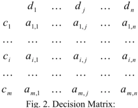
Document classification may be seen (Sebastiani, 2002) as the task of determining an assignment of a value from to each entry of the decision matrix: where g is a set of predefine categories, and is a set of documents to be classified.
}
1
,
0
{
}
,
{
c
1,c
mC
=
K
}
,
{
d
1,d
nD
=
K
n m j m m m n i j i i i n j n ja
a
a
c
a
a
a
c
a
a
a
c
d
d
d
, , 1 , , , 1 , , 1 , 1 1 , 1 1 1K
K
K
K
K
K
K
K
K
K
K
K
K
K
K
K
K
K
K
K
Fig. 2. Decision Matrix:
A value of 1 for is interpreted as a decision to file under and a value of 0 is interpreted as a decision not to file under .
j i
a
, jd
c
i jd
c
iFor understanding this task some observations can be made:
• the categories are just symbolic labels. No additional knowledge of their “meaning” is available to help in the process of building the classifier in particular, this means that the “text” constituting the label (e.g. Sports in a news classification task) cannot be used;
• the attribution of documents to categories should, in general, be attributed on the basis of the content of the documents, and not on the basis of metadata (e.g. publication date, document type, etc.) that may be available from an external source. This means that the
notion of relevance of a document to a category is inherently subjective.
Different constraints may be enforced on the classification task, depending on the application: 1.
{
≤
1
|
1
|
≥
1
|
K
}
elements of C must beassigned to each element of D. When exactly one category is assigned to each document, this is often referred to as the non-overlapping categories case.
2. each element of C must be assigned to
}
|
1
|
1
|
1
{
≤
≥
K
elements of D.A number of distinguishable activities fall under the general heading of classification, but here is a list of the main types, with sample applications attached for illustrative purposes. The aim here is not to say how such problems should be solved, but to identify the main issues.
– Routing. An online information provider sends one or more articles from an incoming news feed to a subscriber. This is typically done by having the user write a standing query that is stored run against the feed at regular intervals, e.g., once a day. This can be viewed as a categorization task, to the extent that documents are being classified into those relevant to the query and those which are not relevant. But a more interesting router would be one that split a news feed into multiple topics for further dissemination.
– Indexing. A digital library associates one or more index terms from a controlled vocabulary with each electronic document in its collection. Wholly manual methods of classification are too onerous for most online collections, and information providers are faced with a large number of difficult decisions to make regarding how to deploy technology to help. Even if an extant library classification scheme is adopted, such as MARC4 or the Library of Congress Online Catalog, there remains the issue of how to provide human classifiers with automatic assistance.
– Sorting. A knowledge management system clusters an undifferentiated collection of memos or email messages into a set of mutually exclusive categories.
Since these materials are not going to be indexed or published, a certain level of error can be tolerated. It is obvious that some of these documents will be easier to cluster than others. For example, some may be extremely short, yielding few clues to their content; some may be on one topic, while others cover multiple topics. In any event, there will be outliers, which will need to be dealt with by manual cleanup, if a high degree of classification accuracy is really necessary.
– Supplementation. A scientific publisher associates incoming journal articles with one or more sections of a digest publication where new results should be cited. Even if authors have been asked to supply keywords, matching those keywords to the digest classification may be nontrivial. However, there may be many clues to where an article goes, over and above the actual scientific content of the paper. For example, the authors may each have previously published work that has already been classified. Also, their paper may cite works that have already been classified. Leveraging this metadata will be the key to any degree of automation applied to this process. – Annotation. A legal publisher identifies the points of law in a new court opinion, writes a summary for each point, and classifies the summaries according to a preexisting scheme. Given the volume of case law, these tasks are most likely performed by teams of people. The written summaries will not be very long, and so any automatic means of classification will not have much text to work with. However, each summary comes from a larger text, which may yield clues as to how the summaries should be classified. It is possible that simply having program route new summaries to the right classification expert would improve the workflow (Jackson and Moulinier, 2002).
2.1. Evaluating Text Classifiers
There are several criteria (Chakrabarti, 2003) to evaluate classification systems:
- Accuracy, the ability to predict the correct class labels most of the time. This is based on comparing the classifier-assigned labels with human-assigned labels.
- Speed and scalability for training and applying/testing in batch mode.
- Simplicity, speed, and scalability for document insertion, deletion, and modification, as well as moving large sets of documents from one class to another.
- Ease of diagnosis, interpretation of results, and adding human judgment and feedback to improve the classifier.
3. ALGORITHMS USED FOR TEXT CATEGORIZATION
3.1. Handcrafted rule based methods
In the '80s (Sebastiani, 2002) the most popular approach (at least in operational settings) for the creation of automatic document classifiers
consisted in manually building, by means of knowledge engineering techniques, an expert system capable of taking text classification decisions. Such an expert system would typically consist of a set of manually defined logical rules, one per category, of type
if <DNF formula> then <category>
A DNF (disjunctive normal form) formula is a disjunction of conjunctive clauses; the document is classified under <category> if it satisfies the formula, if it satisfies at least one of the clauses. The most famous example of this approach is the Construe system built by Carnegie Group for the Reuters news agency. A sample rule of the type used in Construe is illustrated in figure 1.
Figure 1. Rule-based classifier for the Wheat category; keywords are indicated in italic, categories are indicated in caps.
However, it can readily be appreciated that the handcrafting of such rule sets is a non-trivial undertaking for any significant number of categories. The Construe project ran for about 2 years, with 2.5 person-years going into rule development for the 674 categories. The total effort on the project prior to delivery to Reuters was about 6.5 person-years (Jackson and Moulinier, 2002). The drawback of this approach is the knowledge acquisition bottleneck well-known from the expert systems literature. That is, the rules must be manually defined by a knowledge engineer with the aid of a domain expert (in this case, an expert in the membership of documents in the chosen set of categories): if the set of categories is updated, then these two professionals must intervene again, and if the classifier is ported to a completely different domain (set of categories) a different domain expert needs to intervene and the work has to be repeated from scratch (Sebastiani, 2002).
3.2. Linear classifiers
Classifiers are modeled as separators in a metric space. It assumes that documents can be sorted into two mutually exclusive classes, so that a document either belongs to a category, or it does not. The classifier corresponds to a hyper plane (or a line) separating the positive examples from the negative examples. If the document falls on one side of the line, it is deemed to belong to the category; if it falls on the other side of the line, it does not. Classification error occurs when a document ends up on the wrong side of the line.
Linear separation in the document space
A linear separator can be represented by a vector of weights in the same feature space as the documents. The weights in the vector are learned using training data. The general idea is to move the vector of weights towards the positive examples, and away from the negative examples.
The documents are represented as feature vectors. Features are typically words from the collection of documents. Some methods have used phrasal structures, or sequence of words as features, although this is less common. The components of a document vector can be 0 or 1, to indicate presence or absence, or they can be a numeric value reflecting both the frequency of the feature in the document and its frequency in the collection. The familiar tf-idf weight is often used.
When a new document is classified, we look to see how close this document is to the weight vector. If the document is ‘close enough’, it is classified to the category. The score of this new document is evaluated by computing the dot product between the vector of weights and the document.
Formally, if a document, D, is represented as the document vector
d
r
=
(
d
1,
d
2,...,
d
n)
and the vector of weightsC
r
=
(
w
1,
w
2,...,
w
n)
represents the classifier for class C, then the score of document D for class C is computed by:∑
=⋅
=
⋅
=
n i i i CD
d
C
w
d
f
1)
(
r
r
The computed score is a numeric value, rather than being a binary ‘yes/no’ indicator of membership. The most commonly used method to decide whether document D belongs to class C given that score is to set a threshold θ, Then if
θ
≥
)
(
D
f
C ,we decide that the document is ‘close enough’ and assign it to the class (Jackson and Moulinier, 2002).
Rocchio's algorithm
Rocchio is the classic method for document routing or filtering in information retrieval. In this method, a prototype vector is built for each class , and a document vector D is classified by calculating the distance between D and each of the prototype vectors.
j
c
The distance can be computed by for instance the dot product or by using the Jaccard similarity measure.
The prototype vector for class is computed as the average vector over all training document vectors that belong to class . This means that learning is very fast for this method (Aas and Eikvil, 1999).
j
c
j
c
The algorithm consists of applying the formula shown below to the current weight vector, W, to produces a new weight vector, W. Typically, the first weight vector will have all zero components, unless there is prior knowledge of the class, e.g., in terms of keywords that have already been assigned. The jth component of the new weight vector, ,
is: j
w
C C D j C C D j j jn
n
d
n
d
w
w
−
−
+
′
=
α
β
∑
∈γ
∑
∉ ,where n is the number of training examples, C is the set of positive examples (all training documents assigned to the class) and nC is the number of examples in C. dj is the weight of the jth feature in document D. α, β and γ control the relative impact of the original weight vector, the positive examples, and the negative examples respectively.
Rocchio’s algorithm is often used as a baseline in categorization experiments. One of its drawbacks is that it is not robust when the number of negative instances grows large.
3.3. On-line learning algorithms
On-line learning algorithms, encounter examples singly and adapt weights incrementally, computing small changes every time a labeled document is presented. In general terms, on-line algorithms run through the training examples one at a time, updating a weight vector at each step. The weight vector after processing the ith example is denoted by
w
r
i=
(
w
i,1,
w
i,2,...,
w
i,n)
. At each step, the newvector,
w
r
i+1, is computed from the old weight vector,w
r
iusing training examplex
r
iwith label yi. For all methods, the updating rule aims at promoting good features and demoting bad ones. Once the linear classifier has been trained, we can classify new documents using , the final weight vector. Alternatively, if we keep all weight vectors, we can use the average of these weight vectors, which was reported to be a better choice:1
+
n
w
r
∑
=+
=
n i iw
n
w
11
1
r
r
When we want to train classifiers on-line, we need to choose how and when weights are updated.
Widrow-Hoff algorithm
The Widrow-Hoff algorithm, also called Least Mean Squared, updates weights by making a small move in the direction of the gradient of the square loss,
(
w
r
i⋅
x
r
i−
y
i)
2. It typically starts with allweights initialized to 0, although other settings are possible. It then uses the following updating rule:
j i i i i j i j i
w
w
x
y
x
w
+1,=
,−
2
η
(
r
⋅
r
−
)
,This rule is obtained by taking the derivative of the loss function introduced above,
η
is the learning rate, which controls how quickly the weight vector is allowed to change, and how much effect each training example has on the weight vector.The weight-updating rule is applied to all features, and to every example, whether the example is misclassified by the current linear classifier or not. On-line learning of linear classifiers produces adaptive classifiers, classifiers that can learn on the fly. These classifiers are very simple, but effective and easy to train. Update rules are also simple and efficient, although a complex document representation may use a lot of space (Jackson and Moulinier, 2002).
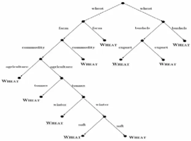
3.4. Decision tree classifiers
A decision tree text classifier is a tree in which internal nodes are labeled by terms, branches departing from them are labeled by tests on the weight that the term has in the test document, and leafs are labeled by categories. Such a classifier categorizes a test document by recursively testing for the weights that the terms labeling the internal nodes have in vector , until a leaf node is reached; the label of this node is then assigned to
j
d
j
d
r
j
d
. Most such classifiers use binary document representations, and thus consist of binary trees. An example decision tree is illustrated in Figure 2. A possible method for learning a decision tree for category consists in a “divide and conquer” strategy of:i
c
- checking whether all the training examples have the same label (either
c
i orc
i);- if not, selecting a term , partitioning Tr into classes of documents that have the same value for , and placing each such class in a separate subtree. The process is recursively repeated on the subtrees until each leaf of the tree so generated contains training examples assigned to the same category , which is then chosen as the label for the leaf. The key step is the choice of the term on which to operate the partition, a choice which is generally made according to an information gain or entropy criterion. However, such a fully grown tree may be prone to overfitting, as some branches may be too specific to the training data.
k
t
kt
ic
kt
Figure 2. A decision tree. (edges are labeled by terms and leaves are labeled by categories; underlining denotes negation)
Most decision tree learning methods thus include a method for growing the tree and one for pruning it, for removing the overly specific branches. Variations on this basic schema for DT learning abound.
3.5. Decision rule classifiers
A classifier for category built by an inductive rule learning method consists of a disjunctive normal form rule, a conditional rule with a premise in disjunctive normal form. The literals in the premise denote the presence or absence of the keyword in the test document , while the clause head denotes the decision to classify under . Decision rules are similar to decision trees in that they can encode any Boolean function. However, an advantage of decision rule learners is that they tend to generate more compact classifiers than decision tree learners.
i
c
jd
jd
c
iRule learning methods usually attempt to select from all the possible covering rules (rules that correctly classify all the training examples) the “best” one according to some minimality criterion. While decision trees are typically built by a top-down, “divide-and-conquer” strategy, decision rules are often built in a bottom-up fashion. Initially, every training example is viewed as a clause j
d
i nγ
η
η
η
1,
2,...,
→
whereη
1,
η
2,...,
η
n are the terms contained ind
jandγ
i equalsc
i orc
i according to whether is a positive or negative example of . The learner applies then a process of generalization in which the rule is simplified through a series of modifications (removing premises from clauses, or merging clauses) that maximize its compactness while at the same time not affecting the “covering” property of the classifier. At the end of this process, a “pruning” phase similar in spirit to that employed in decision trees is applied, where the ability to correctly classify all the training examples is traded for more generality (Sebastiani, 2002).j
d
i
c
3.6. Naïve Bayes classifier
The naive Bayes classifier is constructed by using the training data to estimate the probability of each class given the document feature values of a new instance. We use Bayes theorem to estimate the probabilities:
)
(
)
|
(
)
(
)
|
(
d
P
c
d
P
c
P
d
c
P
j j j=
The denominator in the above equation does not differ between categories and can be left out. Moreover, the naive part of such a model is the assumption of word independence, we assume that the features are conditionally independent, given the class variable.
This simplifies the computations yielding
∏
==
M i j i j jd
P
c
P
d
c
c
P
1)
|
(
)
(
)
|
(
An estimate for can be calculated from the fraction of training documents that is assigned to class :
)
(
ˆ
jc
P
P
(
c
j)
jc
N
N
c
C
P
j j=
=
)
(
ˆ
Moreover, an estimate for is given by:
)
|
(
ˆ
j ic
d
P
P
(
d
i|
c
j)
∑
=+
+
=
M k kj ij j iN
M
N
c
d
P
11
)
|
(
ˆ
where is the number of times word i occurred within documents from class in the training set.
ij
N
j
c
Despite the fact that the assumption of conditional independence is generally not true for word appearance in documents, the Naive Bayes classifier is surprisingly effective (Aas and Eikvil, 1999).
3.7. k Nearest Neighbors (kNN)
k-NN is a memory based classifier that learns by simply storing all the training instances. During prediction, k-NN first measures the distances between a new point x and all the training instances, returning the set N(x,D, k) of the k points that are closest to x. For example, if training instances are represented by real-valued vectors x, we could use Euclidean distance to measure the distance between x and all other points in the training data, i.e.
||
x
−
x
i||
2 i = 1, . . . , n. After calculating the distances, the algorithm predicts a class label for x by a simple majority voting rule using the labels in the elements of N (x, D, k), breaking ties arbitrarily. In spite of its apparent simplicity, k-NN is known to perform well in many domains. In the case of text, majority voting can be replaced by a smoother metric where, for each classc, a scoring function
∑
∈ ′′
=
) , , ()
,
cos(
)
|
(
k D x N x Cx
x
x
c
s
is computed through vector-space similarities between the new documents and the subset of the k neighbors that belong to class c, where
is the subset of
containing only points of class c. Despite the simplicity of the method, the performance of k-NN in text categorization is quite often satisfactory in practice (Pierre, Paolo and Padhraic, 2003).
)
,
,
(
x
D
k
N
CN
(
x
,
D
,
k
)
3.8. Support Vector Machines (SVM) classifiers
Support Vector Machines is a relatively new learning approach introduced by Vapnik in 1995 for solving two-class pattern recognition problems. It is based on the Structural Risk Minimization principle for which error-bound analysis has been theoretically motivated. The method is defined over
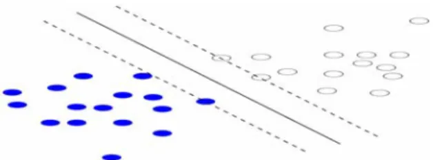
a vector space where the problem is to find a decision surface that “best” separates the data points in two classes. In order to define the “best” separation, we need to introduce the “margin” between two classes. Figures 3 and 4 illustrate the idea. For simplicity, we only show a case in a two-dimensional space with linearly separable data points, but the idea can be generalized to a high dimensional space and to data points that are not linearly separable. A decision surface in a linearly separable space is a hyperplane.
Figure 3. A decision line (solid) with a smaller margin which is the distance between the two parallel dashed lines.
Figure 4. The decision line with the maximal margin. The data points on the dashed lines are the Support Vectors.
The solid lines in figures 3 and 4 show two possible decision surfaces, each of which correctly separates the two groups of data. The dashed lines parallel to the solid ones show how much one can move the decision surface without causing misclassification of the data. The distance between each set of those parallel lines is referred to as “the margin”. The SVM problem is to find the decision surface that maximizes the margin between the data points in a training set.
More precisely, the decision surface by SVM for linearly separable space is a hyperplane which can be written as
0
=
−
⋅
x
b
w
r
r
x
r
is an arbitrary data point (to be classified), and the vector and the constant b are learned from a training set of linearly separable data. Lettingdenote the training set, and be the classification for (+1for being
a positive example and -1 for being a negative example of the given class), the SVM problem is to find
w
r
)}
,
{(
y
ix
iD
=
r
}
1
{
±
∈
iy
x
r
w
r
and b that satisfies the following constraints1
for
,
1
=
+
+
≥
−
⋅
x
b
y
iw
r
r
1
for
,
1
=
−
−
≤
−
⋅
x
b
y
iw
r
r
and that the vector 2-norm of
w
r
is minimized. The SVM problem can be solved using quadratic programming techniques. The algorithms for solving linearly separable cases can be extended for solving linearly non-separable cases by either introducing soft margin hyperplanes, or by mapping the original data vectors to a higher dimensional space where the new features contains interaction terms of the original features, and the data points in the new space become linearly separable.An interesting property of SVM is that the decision surface is determined only by the data points which have exactly the distance from the decision plane. Those points are called the support vectors, which are the only effective elements in the training set; if all other points were removed, the algorithm will learn the same decision function.
||
||
/
1
w
r
This property makes SVM theoretically unique and different from many other methods (Yang and Liu, 1999).
3.9. Feature Selection
Even methods like SVMs that are especially well suited for dealing with high dimensional data (such as vectorial representations of text) can suffer if many terms are irrelevant for class discrimination. Feature selection is a dimensionality reduction technique that attempts to limit overfitting by identifying irrelevant components of data points and has been extensively studied in pattern recognition and in machine learning.
Methods essentially fall into one of two categories: filters and wrappers. Filters attempt to determine which features are relevant before learning actually takes place. Wrapper methods, on the other hand, are based on estimates of the generalization error computed by running a specific learning algorithm and searching for relevant features by minimizing the estimated error. Although wrapper methods are in principle more powerful, in practice their usage is often hindered by the computational cost. Moreover, they can overfit the data if used in conjunction with classifiers having high capacity (Pierre, Paolo and Padhraic, 2003).
4. MEASURES OF PERFORMANCE
The performance of a hypothesis function h(·) with respect to the true classification function f (·) can be measured by comparing h(·) and f (·) on a set of documents Dt whose class is known (test set). In the case of two categories, the hypothesis can be completely characterized by the confusion matrix (figure 5):
Figure 5. Confusion matrix for two case scenarios. where TP, TN, FP, and FN mean true positives, true negatives, false positives, and false negatives, respectively. In the case of balanced domains (i.e. where the unconditional probabilities of the classes are roughly the same) accuracy A is often used to characterize performance. Accuracy is defined as
|
|
D
tTP
TN
A
=
+
Classification error is simply E = 1−A. If the domain is unbalanced, measures such as precision and recall are more appropriate. Assuming (without losing generality) that the number of positive documents is much smaller than the number of negative ones, precision is defined as
FP
TP
TP
+
=
π
and recall is defined asFN
TP
TP
+
=
ρ
.A complementary measure that is sometimes used is specificity
FN
TN
TN
+
=
σ
.In the case of multiple categories we may define precision and recall separately for each category c, treating the remaining classes as a single negative class. Interestingly, this approach also makes sense in domains
where the same document may belong to more than one category. In the case of multiple categories, a single estimate for precision and a single estimate for recall can be obtained by averaging results over classes. Averages, however, can be obtained in two ways. When microaveraging, correct classifications are first summed individually:
c K c c K c c
FP
TP
TP
+
=
∑
∑
= = 1 1 µπ
, c K c c K c c cFN
TP
FP
TP
+
+
=
∑
∑
= = 1 1 µρ
When macroaveraging, precision and recall are averaged over categories:
∑
==
K c c MK
11
π
π
,∑
==
K c c MK
11
ρ
ρ
Compared to microaverages, macroaverages tend to assign a higher weight to classes having a smaller number of documents.
5. CONCLUSIONS
This paper has presented an overview of basic formulations and approaches to classification. It presented the algorithms that can be used in text classification: handcrafted rules, decision trees, decision rules, on-line learning, linear classifier, Rocchio algorithm, k Nearest Neighbor (kNN), Support Vector Machines (SVM).
REFERENCES
Aas, K. and L. Eikvil (1999), Text categorisation: A survey, Norwegian Computing Center.
Chakrabarti, S. (2003), Mining the Web: Discovering Knowledge from Hypertext Data, Morgan Kaufmann Publishers, San Francisco, USA.
Jackson, P. and I. Moulinier (2002), Natural Language Processing for Online Applications Text Retrieval, Extraction and Categorization, John Benjamins B.V., Amsterdam, The Netherlands.
Pierre B., F. Paolo and S. Padhraic (2003),
Modeling the Internet and the Web: Probabilistic Methods and Algorithms, JohnWiley & Sons Ltd, West Sussex, England. Sebastiani, F. (2002), A Tutorial on Automated
Text Categorisation, Istituto di Elaborazione dell'Informazione, Consiglio Nazionale delle Ricerche.
Yang, Y. and X. Liu (1999), A re-examination of text categorization methods, 22nd Annual International SIGIR, Berkley, pp. 42-49.