Scalable optimization-based Scheduling approaches for HPC facilities

A

LMA

M

ATER

STUDIORUM

- U

NIVERSITÁ DI

BOLOGNA

D

OTTORATO DI

R

ICERCA IN

C

OMPUTER

S

CIENCE AND

E

NGINEERING

C

: XXX

SETTORE CONCORSUALE DI AFFERENZA 09/H1 SETTORE SCIENTIFICO DISCIPLINAREING-INF/05

Scalable optimization-based

Scheduling approaches for HPC

facilities

Presentata da:

Thomas B

RIDI

Coordinatore Dottorato:

Chiar.mo Prof.

Paolo C

Supervisore:

Chiar.mo Prof.

Michela M

iii

Alma Mater Studiorum - Universitá di Bologna

Abstract

Scalable optimization-based Scheduling approaches for HPC facilities

by Thomas BRIDI

This Thesis deals with the problem of scheduling applications on High-Performance Computing (HPC) machines. The goal is to create a sched-uler that can improve the solutions w.r.t. the state-of-the-art under different metrics. However, improving the solution quality is not enough: creating a scheduler for future HPC machines requires to take into account also over-heads and scalability. In this thesis we present a comprehensive, scalable, scheduling approach that features both an off-line and an on-line component. The off-line component is based on Constraint Programming (CP), an opti-mization technique that is well-suited for scheduling problems and allows for great flexibility. We leverage this flexibility to present first a optimization method designed to optimize the job waiting times, which is then extended via heuristics and search strategies to deal with more complex objective func-tions. Unfortunately, such a complex objective function cannot be handled by a solver in an acceptable amount of time for online operation on a HPC ma-chine in-production. We deal with this difficulty by making use of a second, distributed, on-line scheduler. This second scheduler is designed to dramati-cally decrease the computational overhead and achieve a scalability adequate to future ExaFlops HPC machines. The distributed scheduler is proactive, and it takes decisions so as to follow a desirable, pre-specified, utilization profile. This feature makes it possible to connect these two schedulers to cre-ate a hybrid system: the CP component computes the scheduling on a trace of forecasted jobs one day ahead, machine learning techniques extract from the solution a near-optimal and desirable utilization profile, and the online scheduler takes care of the actual scheduling decisions in a scalable fashion. The resulting architecture manages to improve the HPC machine profit by an average 8.6%, while decreasing the computational overhead and, under normal conditions, without any side effect.

v

List of Pubblications

Part of the work in this thesis have previously appeared in:

1. A. Bartolini, A. Borghesi, T. Bridi, M. Lombardi, and M. Milano. Proac-tive workload dispatching on the EURORA supercomputer. English. In Principles and practice of constraint programming - 20th international conference, CP 2014, lyon, france, september 8-12, 2014. proceedings. B. O’Sullivan, editor. Vol. 8656. In Lecture Notes in Computer Science. Springer. Springer International Publishing, 2014, pp. 765–780. ISBN: 978-3-319-10427-0. DOI: 10.1007/978-3-319-10428-7_55

2. T. Bridi, M. Lombardi, A. Bartolini, L. Benini, and M. Milano. A cp scheduler for high-performance computers. In. Vol. 1485, 2015, pp. 37–42. URL: https : / / www . scopus . com / inward / record . uri ? eid = 2 - s2 . 0 - 85009223255 & partnerID = 40 & md5 = 65ac2e65b77b8fbb06d15c101edd7bbd

3. T. Bridi, A. Bartolini, M. Lombardi, M. Milano, and L. Benini. A con-straint programming scheduler for heterogeneous high-performance computing machines. IEEE transactions on parallel and distributed sys-tems, 27(10):2781–2794, 2016. DOI: 10.1109/tpds.2016.2516997_. URL: http://dx.doi.org/10.1109/TPDS.2016.2516997

4. T. Bridi, M. Lombardi, A. Bartolini, L. Benini, and M. Milano. DARDIS: Distributed And Randomized DIspatching and Scheduling. In Euro-pean conference on artificial intelligence (ECAI 2016). Vol. 285. Gal A. Kaminka et al., 2016, pp. 1598–1599

5. T. Bridi, M. Lombardi, A. Bartolini, L. Benini, and M. Milano. DARDIS: Distributed And Randomized DIspatching and Scheduling. In, AI*IA 2016 advances in artificial intelligence, pp. 493–507. Springer, 2016

6. T. Bridi, A. Bartolini, M. Lombardi, P. V. Hentenryck, M. Milano, and L. Benini. Profit-driven hpc scheduling optimization and pue analysis.

IEEE transactions on industrial informatics, under review, 2017

7. T. Bridi, A. Bartolini, M. Lombardi, M. Milano, and L. Benini. Hybrid offline-optimized and online-distributed profit-driven low-overhead scheduler for hpc with automatic node shut-down and turn-on. IEEE transactions on parallel and distributed systems, under review, 2017

8. C. Galleguillos, A. Sîrbu, Z. Kiziltan, O. Babaoglu, A. Borghesi, and T. Bridi. Data-driven job dispatching in hpc systems. In International workshop on machine learning, optimization, and big data. Springer, 2017, pp. 449–461

vii

Contents

Abstract iii

List of Pubblications v

List of Figures xi

List of Tables xiii

List of Abbreviations xv 1 Introduction 1 1.1 Content . . . 2 1.2 Contribution . . . 4 1.3 Outline . . . 5 2 Related work 7 2.1 HPC systems. . . 7 2.2 HPC scheduling . . . 8 2.2.1 Rule-based. . . 9 2.2.2 Backfilling . . . 10 2.3 HPC scheduling optimization . . . 13 2.4 Distributed scheduling . . . 14

2.5 On HPC energy, profit, and scheduling. . . 16

2.6 Costraint Programming . . . 17

2.6.1 Constraint filtering and propagation . . . 18

2.6.2 Modeling . . . 19

CP modeling for scheduling problems . . . 20

2.6.3 Search strategies . . . 22

3 Preliminary study on the application of CP in HPC scheduling: modeling and simulations 25 3.1 Introduction . . . 25

3.2 System Description and Motivations for Using CP . . . 26

3.3 Design of a CP Approach . . . 28

3.3.1 Formal Problem Definition . . . 28

3.3.2 CP Model . . . 29

3.4 Added Value of CP . . . 32

3.4.1 Evaluation of Our Models . . . 33

3.4.2 Comparison with PBS . . . 35

viii

4 CP in HPC scheduling: a first application and evaluation on the

EU-RORA HPC 41

4.1 The HPC Scheduling problem . . . 43

4.2 Constraint Programming . . . 44

4.2.1 Motivational example . . . 45

4.3 CP Model. . . 47

4.3.1 General model . . . 47

4.3.2 Allocation of jobs within a reservation . . . 49

4.3.3 Feasibility check . . . 50 4.4 Framework architecture . . . 51 4.5 Experimental Results . . . 55 4.5.1 Evaluation setup . . . 56 Simulation-based tests . . . 56 Evaluation on the HPC. . . 57 4.5.2 Test generation . . . 57

Test 0: Behavior at different heterogeneity levels . . . . 59

Test 1: 4 nodes 99 jobs . . . 60

Test 2: 65 nodes 330 jobs . . . 61

Test 3: 65 nodes 700 jobs . . . 62

Results comparison. . . 62

Guidelines for algorithm portfolio selection . . . 63

4.5.3 Execution on Eurora . . . 64

4.5.4 Overhead distribution . . . 66

4.6 Conclusion . . . 71

5 Improving the HPC scheduling scalability with Distributed And Randomized DIspatcher and Scheduler (DARDIS) 73 5.1 Motivational example . . . 75

5.2 Profile aware scheduling . . . 76

5.2.1 Rule-based schedulers for variable profiles . . . 78

5.3 DARDIS approach . . . 78

5.3.1 Scheduling. . . 80

5.3.2 Dispatching . . . 81

5.3.3 Throughput driven DARDIS . . . 82

Backfilling in DARDIS . . . 82

5.3.4 Profile driven DARDIS. . . 83

5.3.5 Balance driven DARDIS . . . 83

5.3.6 Deadline exceeding. . . 84

5.4 Complexity study . . . 84

5.5 Experimental results . . . 85

5.6 Conclusion . . . 88

6 Optimal Profit-driven offline scheduling with cooling optimization 91 6.1 Workflow. . . 92

6.2 Scheduling problem. . . 92

6.3 Rule-based scheduling . . . 93

6.4 ILOG CP Optmizier default search . . . 94

ix

6.5.1 The Model Variables . . . 95

6.5.2 The Constraints . . . 95

6.5.3 The Objective Function . . . 96

6.6 Heuristic for the first solution . . . 97

6.7 Searches . . . 98

6.7.1 Multi-Search . . . 98

6.7.2 Relaxation-Based Search . . . 98

6.7.3 The Delay Search . . . 99

6.8 Results . . . 100

6.8.1 The Test Case . . . 100

6.8.2 The Implementation . . . 103

6.8.3 Profit comparison . . . 104

6.9 Conclusion . . . 106

7 Hybrid Offline-Optimized and Online-Distributed Profit-driven low-overhead scheduler for HPC with automatic node shut-down and turn-on 109 7.1 Scheduling problem. . . 110

7.2 Workflow. . . 111

7.3 Offline CP scheduling . . . 113

7.4 Profile Extraction . . . 114

7.5 Distributed Online scheduling. . . 116

7.6 Results . . . 119 7.6.1 Profit improvement. . . 120 7.6.2 Makespan . . . 120 7.6.3 Overhead . . . 121 7.7 Conclusion . . . 121 8 Conclusion 123 Bibliography 125

xi

List of Figures

2.1 Marconi HPC, Eurora Rack, and Knights-Landing Node . . . 8

2.2 Scheduling example per and post Backfilling . . . 11

2.3 Filtering and propagation example . . . 19

2.4 Example of cumulative . . . 21

3.1 EURORA utilization on the first trace (BATCH1) . . . 35

3.2 Waiting jobs and queue time for BATCH1 . . . 35

3.3 EURORA utilization on the second trace (BATCH2) . . . 36

3.4 Waiting jobs and queue time for BATCH2 . . . 38

3.5 EURORA utilization on the third trace (BATCH3) . . . 38

3.6 Waiting jobs and queue time for BATCH3 . . . 39

4.1 Feasibility check subdivision . . . 50

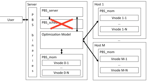
4.2 Framework macro architecture . . . 52

4.3 Workflow. . . 53

4.4 Test Generation . . . 58

4.5 Mean overhead at different heterogeneity levels . . . 60

4.6 Weighted queue time gain w.r.t. PBSFifo . . . 63

4.7 Average queue time gain w.r.t. PBSFifo . . . 64

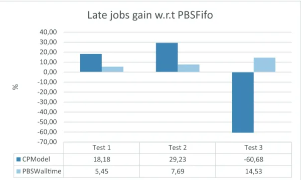
4.8 Number of jobs in late gain w.r.t. PBSFifo . . . 65

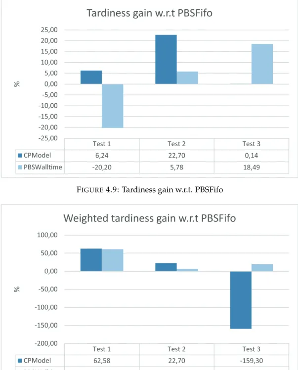
4.9 Tardiness gain w.r.t. PBSFifo . . . 66

4.10 Weighted tardiness gain w.r.t. PBSFifo . . . 66

4.11 Maximum overhead gain w.r.t. PBSFifo . . . 67

4.12 Overhead percentage on execution time gain w.r.t. PBSFifo . . 68

4.13 Working ranges . . . 68

4.14 Weighted queue time extrapolated from Eurora. . . 69

4.15 Core utilization on Eurora . . . 69

4.16 Overhead distribution for the simulated test . . . 70

4.17 Overhead distribution for Eurora . . . 70

5.1 Example of a profile aware scheduling architecture. . . 77

5.2 DARDIS architecture . . . 80

5.3 DARDIS results comparison . . . 88

6.1 Workflow of the interaction between the proposed scheduler and the DARDIS scheduler . . . 93

6.2 Percentage of improvement at submission end w.r.t. the best rule based scheduler for the High workload scenario . . . 100

6.3 Percentage of improvement at submission end w.r.t. the best rule based scheduler for the Low workload scenario . . . 101

xii

6.4 Tests makespan for the High workload scenario . . . 102 6.5 Classification tree for the efficiency . . . 102 6.6 Daily PUE and trend for the Delay-Search and the best

Rulebased in the High workload case for the scenarios: (a) Air -Expensive - Summer, (b) Hybrid - -Expensive - Summer, (c) Air Expensive Winter, (d) Hybrid Expensive Winter, (e) Air -Cheap - Summer, (f) Hybrid - -Cheap - Summer, (g) Air - -Cheap - Winter, and (h) Hybrid - Cheap - Winter . . . 103 6.7 PUE at different external temperatures and Slope change

workload in: (a) winter - air cooling, (b) summer - air cooling, (c) winter - hybrid cooling, and (d) summer - hybrid cooling from the results by [99] . . . 105 6.8 Distance from Slope change points at different system

utiliza-tion percentage with efficiency predicutiliza-tion . . . 107 6.9 Efficiency prediction errors . . . 107 7.1 Workflow of the interaction between the Offline CP scheduler,

Profile Extractor, and the online DARDIS scheduler . . . 112 7.2 Profit improvement by DARDIS100%, DARDIS70%, and

DARDIS50% w.r.t the best Rule-based scheduler in the sce-nario. (a) Summer temperature, Air cooling; (b) Summer tem-perature, Hybrid cooling; (c) Winter temtem-perature, Air cooling; (d) Winter temperature, Hybrid cooling. . . 115 7.3 Average makespan obtained by DARDIS100%, DARDIS70%,

DARDIS50%, and the best Rule-based with standard devia-tion. (a) Low workload trace; (b) Medium workload trace; (c) High workload trace. . . 116 7.4 Average overhead with standard deviation, in seconds, at

dif-ferent workload for (a) DARDIS100%, (b) DARDIS70%, (c) DARDIS50%, and (d) the best Rule-based. . . 117

xiii

List of Tables

3.1 Access requirements and waiting times for the PBS queues in

EURORA . . . 28

3.2 An example of problem instance . . . 32

3.3 A feasible solution for the instance from Table 3.2 . . . 32

3.4 Models comparison, queue times . . . 33

3.5 Models comparison, system load . . . 33

3.6 Job traces composition . . . 34

4.1 Node test setup . . . 45

4.2 Jobs set for test 1. . . 45

4.3 PBS by GPUs solution to test 1 . . . 45

4.4 PBS by Walltime and optimization model solution to test 1 . . 46

4.5 Test 1 statistics . . . 46

4.6 Jobs set for test 2. . . 46

4.7 PBS by GPUs and optimization model solution to test 2 . . . . 46

4.8 PBS by Walltime solution to test 2 . . . 47

4.9 Test 2 statistics . . . 47

4.10 Eurora jobs utilization . . . 59

4.11 GPUs & MICs per node request distribution on Eurora . . . . 59

4.12 Memory per node request distribution on Eurora . . . 60

4.13 Simulated test with 4 nodes and 99 jobs . . . 61

4.14 Simulated test with 65 nodes and 330 jobs . . . 61

4.15 Simulated test with 65 nodes and 700 jobs . . . 62

4.16 Optimization model average overheads (seconds) . . . 67

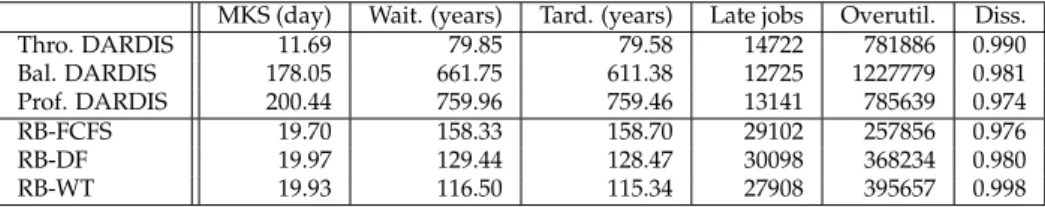
5.1 Results obtained by DARDIS and rule-based schedulers on 300 nodes and 35538 jobs scheduling . . . 87

5.2 Overhead comparison of DARDIS and rule-based scheduler in seconds . . . 88

6.1 Example of PUE table. . . 97

6.2 PUE efficiency in each scenario for ILOG, the proposed strate-gies, the best Rule-based scheduler, and Slope change . . . 101 7.1 DARDIS70% Vs. RB percentile profit improvement comparison 114

xv

List of Abbreviations

AI ArtificialIntelligence

CP ConstraintProgramming

CSP ConstraintSatisfactionProblem

DARDIS DistributedAndRandomizedDIspatcher andScheduler

FLOPS FLoating pointOperationsPerSecond

HPC HighPerformanceComputing

LNS LargeNeighborhoodSearch

MPI MessagePassingInterface

NFS NetworkFileSystem

OpenMP Open MultiProcessing

PBS PortableBatchScheduler

PUE PowerUsageEffectiveness

RCP RemoteCoPy

RCPSP Resource-ConstrainedProjectSchedulingProblem

SCP SecureCoPy

1

Chapter 1

Introduction

This thesis studies the job scheduling and dispatching problem for High-Performance Computing (HPC) machines.

In these systems achieving a 1% improvement brings substantial advan-tages in terms of money, waiting time and power savings.

HPC machines peak performance, measured in FLOPs (floating point op-eration per second), has been continuously growing since their introduction in 1963 of TOP500 [9] ranking. From 1963 to nowadays the #1 performance for the Linpack benchmark [10] grown from 59.7GFlops to 93PFlops and it is expected that the Exascale (1EFlops) [11] will be reached around the year 2020.

Due to the enormous amount of investments done for these computing machines and the fast depreciation (3-5 years), the return of investment is one of the most important points to keep in mind in both hardware and software and also the scheduler can be set to be profit aware. However, also the user experience is important in these systems. For this reason, we have to consider also other metrics like job waiting time and number of late jobs.

With the new goal of the Exascale, a set of new opportunities comes to the scientific and industrial communities but this brings also a set of new challenges. The first one is the scalability. To create an ExaFlops computer two paths can be taken: the first is to create more computationally powerful nodes, the second is to create HPC with a higher number of nodes. For the first path, the problem is that the integrated circuit density limit is going to be reached an this will limit the computational power of a single chip [12]. For this reason, the most affordable way for the Exascale is to substantially increase the number of computational nodes into an HPC machine. This brings scalability problems both in the hardware and the software: starting from the nodes interconnections to the application scalability and even to the scheduler.

A second problem comes from a power limitation. Usually, energy providers fix the power limit for industrial buildings to 20MW. This limit is valid also for computing centers. The current #1 in the TOP500 list, the Sun-way TaihuLight, can provide a computing power of 93PFlops with a power consumption of 15.37MW. This means that for the future Exascale machines, the engineers have to increase the computational power 10 times w.r.t. the current top HPC with an increment of the consumption of 0.3 times.

In this scenario the importance of the scheduler is pervasive. With an appositely designed scheduler, it is possible to not just to improve the system

2 Chapter 1. Introduction

utilization and the user experience with highly scalable algorithms but also to improve the system efficiency in order to decrease the power consumption, anticipate the return of investments, increase the profit and create a greener computing system.

This results cannot be achieved just by a single approach like greedy and heuristic algorithms or distributed computing or optimization techniques but by a hybrid approach that exploits all of them.

The focus of the thesis is on the optimization of the scheduling results under several different metrics and the scalability to make this optimization usable in a real environment. HPC machines (also called supercomputers) are computer composed by a set of nodes connected by a network. Each node contains a set of resources (processors, accelerators, memory, etc.). The scheduling problem for HPC consist of a non-preemptable batch scheduling. Jobs are submitted to a high-level scheduler by the user, usually, through a lo-gin node of the machine. The scheduler reacts to the events like submissions and job terminations and tries to schedule and dispatch the waiting jobs. The scheduler selects the node(s) and the starting time for the job execution. It has to deal with resource requirements of the jobs and the available resources of the machine. This means that the scheduler reserves the resources to a job un-til its termination. This is an intentional behavior by the HPC administrator used to prevent preemption on the resources that would lead to performance worsening due to cache replacement and context switching. The objective of the scheduler is to optimize different metrics (depending on the needs of the computing center) as for example user’s related metrics as waiting times, throughput, etc. From now on we refer to scheduling and dispatching as scheduling.

Job dispatching in supercomputers is a special case of the wider Schedul-ing and Allocation problem that arises in several different computSchedul-ing fields.

1.1

Content

This thesis deals with the job scheduling and dispatching problem in HPC systems which can be subdivided into two components:

1. the allocation problem: choosing the set of nodes to be assigned to each job

2. the scheduling problem: deciding the start time for each job avoiding resource overusage.

Our attention is directed to the scalability and the profitability of the scheduler. The idea is to create a highly scalable scheduler that can also im-prove the profit of a computing center. In fact, the content of this work can be subdivided into five different points:

A preliminary study on the application of Constraint Programming to the HPC scheduling problem We study the applicability of Constraint Pro-gramming to the HPC scheduling problem. We model the basic features of

1.1. Content 3

an HPC scheduler. The experimentations in this study demonstrated the fea-sibility of the approach and showed promising results w.r.t. the commercial scheduler PBS Professional 12. However, not all the features required for an in-production HPC have been taken into account.

A real-word CP scheduler We have developed a second approach, mod-eling the majority of the needed features for an in-production HPC such as arrays of jobs, “critical-priority” jobs, heterogeneous jobs, reservations, etc. Many techniques have been adopted to limit the computational overhead to an acceptable value. Finally, the scheduler has been embedded into a com-mercial scheduler: PBS Professional 12. Further experimentation shows that the approach is still feasible and can improve the results obtained by PBS in terms of makespan and waiting time but with scalability problems. More-over, an experimentation on a real, in-production, HPC has been done with promising results in terms of system utilization.

A distributed and randomized scheduler (DARDIS) This new ing approach for HPC has been designed to drastically decrease the schedul-ing overhead and increase the scalability of the scheduler. The scheduler is designed to distribute the start time selection computation through the nodes while the dispatching is done by the job itself on the basis of the can-didate starting times returned by the nodes. Results show that just in some cases it can improve the results obtained by commercial schedulers while the scheduling computation is 10 times faster.

A profit-aware offline scheduler This CP scheduler is an offline scheduling solution designed to optimize the profit obtained from the HPC consider-ing not only the set of submitted jobs and the resources but also the coolconsider-ing model and the external temperature forecast. The scheduler is designed to schedule synthetic jobs or the set of jobs submitted in the last 24h, obtain a sub-optimal utilization profile optimizing the profit. This profile is then sent to a profile-aware online scheduler. Moreover, this study also provides an analysis on the system efficiency to decide if to increase or decrease the workload of the next day to improve the profit. Experimentations in sev-eral different scenarios have been done considering: different external tem-peratures, cooling models, pricing schema, etc. It has been shown that the scheduler achieves profit improvements up to 6-7% w.r.t. standard and ad-hoc rule-based schedulers in the case of high-workload while no worsening have been found in case of low workload.

A hybrid offline-online scheduler This scheduler is designed to combine the near-optimal results obtained by optimization techniques such as Con-straint Programming with a fast and scalable distributed scheduler. The scheduler is capable to plan the resources utilization in the future giving the possibility to turning on and off nodes of the system without any de-lay. The scheduler proved to improve the HPC machine profit by on average

4 Chapter 1. Introduction

of a 8.6%. The scheduler also proved to be more scalable of both commer-cial heuristic schedulers and optimized CP schedulers. Moreover, no signifi-cant makespan improvement has been found in the case of low and medium workload requests. However, an increment of 10% in makespan has been found in case of high workload. This worsening is nature of the distributed scheduler.

1.2

Contribution

In this work, we use techniques as Constraint Programming, Distributed sys-tems, and Heuristics. Our contribution consists of the creation of several different schedulers for HPC and analysis on the cooling efficiency of these systems and how to modulate the future system utilization to increase the profit. More in detail, our contribution can be summarized as follows:

• An online Constraint Programming scheduler [1, 3] that models all the different features needed for a commercial scheduler. This scheduler aims to minimize several different metrics such as the makespan, the number of late jobs and the waiting time but the best results have been obtained with the goal of minimizing the weighted queue time. The weighted queue time is a metric designed to take into account the wait-ing time of jobs in a fair way: each waitwait-ing is weighted on the expected waiting of the user.

• A distributed, randomized, and profile-aware scheduler [4, 5]. This scheduler is designed to dramatically improve the scalability of the state-of-the-art schedulers. This is the first distributed scheduler that enables the agent’s agreement without a handshake or an agreement protocol. Moreover, this scheduler is shown to highly decrease the com-putational overhead for the scheduling and dispatching components.

• An offline and profit-aware Constraint programming scheduler [6]. This scheduler models both the HPC resources and the cooling of the system to optimize the scheduling to maximize the profit taking into account the weather forecast. This scheduler has proven to increase the profit of the system up to a 7% in case of high workload while no profit decrement has been found in case of low workload. Moreover, the re-sults of this scheduler have been used to understand when it is more profitable for the system to increase or decrease the system utilization to improve the profit. This lead to a simple rule to forecast which is the best behavior of the scheduler for the next 24h to maximize the profit.

• A hybrid Online-Offline scheduling architecture [7]. This architecture is composed by an offline scheduler capable to optimize the profit of a chunk of jobs. This scheduler is triggered at fixed time intervals (24-48 hours) and, on the basis of a forecasted workload traces, it computes the optimal allocation. The scheduling solution obtained by the offline scheduler is then passed to a “desirable utilization profile generator”

1.3. Outline 5

that generates a utilization profile that contains the schedule of jobs along with node shut down and start up. The desirable utilization pro-file is then fed to the Online scheduler (DARDIS). The online sched-uler is a fast distributed schedsched-uler designed for scalability. The online distributed scheduler is also designed to follow a desirable utilization profile variable in times planning the scheduling in the future.

1.3

Outline

The thesis is organized as follows.

Chapter2shows an introduction to HPC systems and how they work. It introduces the scheduling problem and shows the main algorithms used in real-life HPC machines. It shows the state of the art in scheduling algorithms, scheduling optimization, distributed scheduling. Finally, it introduces the Constraint Programming (CP) paradigm, how it works, the modeling, and the most used searches in this field.

Chapter 3 shows a preliminary study to the application of CP into the HPC scheduling and dispatching problem. The chapter explains the mod-eling of the scheduling problem on the EURORA HPC at CINECA, the first simulations.

Chapter 4shows a first application of a CP model into a real and online scheduler. In this chapter, we modeled the most majority of the constraints to make our CP scheduler a working prototype. The simulations are made to show the scalability of the scheduler. Moreover, an evaluation on the HPC with a real and in-production workload has been made to show its usability. Chapter5shows a distributed and randomized scheduling approach de-signed to solve the scalability problems of the CP scheduler. Distributed And Randomized DIspatcher and Scheduler (DARDIS) is a scheduler that offloads and parallelizes the scheduling problems to the nodes and the dis-patching and commitment to the user. This approach has shown to be faster than heuristic algorithms but, in some cases, obtaining not good solutions.

Chapter6proposes an offline CP scheduler designed to interact with the DARDIS scheduler in order to improve its solution. The idea is to obtain near-optimal solutions with an offline scheduler (as the one proposed in this chapter) using traces obtained from workload forecast and then to guide the DARDIS decision exploiting the offline solution.

Chapter 7 proposes a hybrid offline CP and online distributed schedul-ing solution. The offline scheduler computes a sub-optimal schedulschedul-ing, op-timizing the profit, every 24 hours with the jobs submitted so far. From its best solution an optimal utilization profile is extracted and used for the next 24 hours into the online scheduler. The online and distributed scheduler (DARDIS) uses the utilization profiles generated from the offline scheduler to turn off and on the HPC resources to decreases the energy expenses.

7

Chapter 2

Related work

This chapter gives a view of the state-of-the-art of the scheduling and dis-patching problem for HPC. The chapter is subdivided into sections: Section 2.1 explains the HPC systems architecture. Section 2.2 explores the com-mercial and heuristic solutions used. Section 2.3 shows the state-of-the-art in the HPC scheduling dispatching problem, focusing on optimization and AI techniques. Section 2.4 explores the distributed scheduling approaches present in literature. Section2.5 shows works not related to the scheduling and dispatching but still interesting for our work. Finally, section2.6shows the Constraint Programming paradigm, the CP problems modeling, and its searches.

2.1

HPC systems

High-Performance Computing is a technology widely used for research and industry when high computational power is needed. Usually, these machines are used for physics and chemistry simulations [13, 14, 15], fluid dynamics [16,17,18], material design [19,20,21], pharmaceutical [22,23,24] and so on. HPC machines are massively parallel machines composed by a set of racks, each one with a set of nodes, each node usually contains multiple multi-cores CPUs, accelerators, and RAM (Figure 2.1). In these systems, looking to the TOP500 ranking [9], the core number lays the range from thou-sands [25] to tens of millions [26] core per HPC. This is translated in a num-ber of nodes in the range from hundreds to millions. The computational power of HPC machines is measured in term of PetaFLOPS [27]. However, the emerging target is to point to the ExaFLOPS [28] for the year 2020. All these nodes are usually interconnected by both Gigabit Ethernet [29] and In-finiBand [30] interconnections. This core, processors, and multi-nodes infrastructure is exploited at its best using usually two computing framework Open Multiprocessing (OpenMP) [31] and Message Passing In-terface (MPI) [32] in a hybrid fashion. Combining both MPI and OpenMP gives the possibility to instantiate multiple parallel tasks on different nodes (thanks to MPI) and in each node multiple threads (thanks to OpenMP). These resources are used without concurrency and preemption to maximize the performance. However, to select the right (free) resources and to execute the jobs, a scheduling and dispatching software is needed.

8 Chapter 2. Related work

FIGURE2.1: Marconi HPC, Eurora Rack, and Knights-Landing

Node

These HPC machines are investment-intensive machines with short de-preciation cycles. An average supercomputer reaches full dede-preciation in three to five years [33]. Hence their utilization has to be aggressively man-aged to produce an acceptable return on investment. Even relatively small improvements in utilization, throughput, and quality of service translate into significant financial gains.

2.2

HPC scheduling

The problem of batch scheduling is well-known and widely investigated [34, 35,36,37].

In the HPC jobs scheduling, we usually have a login node which is the only interface to the web. Through this node, the users can login and ac-cess to a remotely mounted home in which the user can develop and test its code for a limited amount of time. The user then can send its application to the HPC submitting its job to the scheduler. When submitting a job, the user can specify the number of nodes required for the execution (from now calledjob units), the amount of resources for each node (Cores, RAM, GPUs, etc.), the maximum execution time (from now called walltime), the queue (or partition) to submit. There are two different execution modes:

• Normal: in normal mode the user submit a script that executes its job, the script is then accessed into the selected nodes through protocols like NFS [38], scp [39], rcp [40], etc. And then it is executed without the possibility for the user to access to the standard output.

• Interactive: an ssh [41] connection to one of the selected nodes is open to the user. After that, the user can run commands to start a job directly on the node. In this way, the user can interact with the job as it is exe-cuted in its local terminal. If a user submits a job with multiple nodes, it can access the remaining nodes through ssh or it can execute a parallel job specifying the selected nodes through MPI.

After the submission, the scheduler takes care of the jobs selection follow-ing the algorithms and rules chosen by the administrator. Each node is then queried to find the set of nodes with enough free resources to execute all the job units of the job. If the resources are available, the job is executed and the next one is selected.

2.2. HPC scheduling 9

This scheduling problem can be classified as a variant of the Resource-Constrained Projects Scheduling Problem (RCPSP). This kind of problem is a well-studied problem and its complexity have been proven to beNP-Hard

[42,43,44].

Some of the most widespread rule-based scheduling software in HPC fa-cilities are PBS Professional [45], Torque [46], Slurm [47]. PBS Professional and Torque are branches of the original OpenPBS project (as described in [48] and [49]), the first is a commercial software distributed by Altair, the second is an open source version of the original PBS. Slurm is an open source sched-uler: differently from PBS that uses queues, it uses resource partitioning to give a finer management and only one queue. In general, the large majority of commercial schedulers have a greedy component: the proposed heuristic does not explore the solutions space and generates a “good” solution. Nei-ther local nor global optimality can be achieved.

The reader can refer to the works [50,51,52] for good surveys on schedul-ing algorithms used in HPC and computschedul-ing clusters. Most of the algorithms described in these works can be implemented within commercial schedul-ing software by definschedul-ing appropriate “schedulschedul-ing rules” (e.g., the min-min algorithm can be implemented sorting jobs by increasing amount of required resources).

In a wider context, there is a large body of literature on scheduling and al-location for data-center workloads [53,54,55,56] relying on the key assump-tion that partial or complete migraassump-tion of parallel jobs is possible during their execution. Even though supercomputers will reasonably move toward more agile execution models [57,58], the common practice today is that job migra-tion is not allowed, to maximize performance and predictability [59].

2.2.1

Rule-based

Rule-based scheduling is one of the first types of algorithms proposed for the scheduling problem [60,61,62] but is still widely used in HPC [63].

This heuristic algorithm (see Algorithm1) processes jobs and nodes in a given order which is specified via a customized rule (lines 1 and 2). When a job is processed, the scheduler considers each job unit (line 4) and starts querying the system nodes to find a sufficient amount of free resources (lines 5-10). When all job units have a candidate node, the job is started (lines 13-15). If a job cannot be immediately started, two alternative behaviors are possible:

• Strict ordering: This is the most priority conservative approach. If jobi

cannot be started, the scheduler stops and waits for the next termina-tion event to restart the process fromi(lines 17-19).

• Non-strict ordering: This is the most utilization aggressive approach. If jobicannot be executed, the scheduler skips it and tries to schedule job

10 Chapter 2. Related work

Algorithm 1RB(J = list of jobs,N = list of nodes, Rule1 = jobs ordering rule, Rule2 = nodes ordering rule, Strict = true if strict ordering)

1: OJ = Order(J,Rule1) 2: ON = Order(N,Rule2) 3: foreachjobjinOJdo

4: foreach wjob unit inj do

5: foreachnodeninON do

6: foreachdifferent resourcekin the noden do

7: ifthe resource requirement ofj is lower or equal to the free resources ofkthen

8: set the execution of the job unitwof jobj to the noden

9: end if

10: end for

11: end for

12: end for

13: ifall the job units of jobj have a nodethen

14: run the job 15: else

16: clear the nodes of each job unit of jobj

17: if Strict then

18: return

19: end if

20: end if

21: end for

Despite the simplicity and similarity of these two approaches it is im-portant to note that choosing a strict or non-strict ordering can lead to two completely different behaviors. With the strict ordering, the jobs priority is always respected thus leading to a high underutilization of the resources. With the non-strict ordering, the priority is used as a soft constraint thus leading to a higher system utilization at the expenses of the user’s fairness.

Many algorithms have been proposed to obtain a trade-off between these two. The majority of these algorithms start with a Strict-ordering-rule-based algorithm and after the first non-executed job applies a backfilling algorithm.

2.2.2

Backfilling

Backfilling algorithms are algorithms designed to fill resources left unused from the main scheduling algorithm (see figure2.2).

Many variants of the backfilling algorithm have been proposed [64]. However, the most used are Conservative Backfilling and EASY-Backfilling.

The Conservative Backfilling algorithm is designed to increase the sys-tem utilization but paying high attention to the jobs fairness: the algorithm is designed to anticipate a job without delaying any higher priority job (see Al-gorithm2). This requires a data structure to store the entire utilization profile of each resource of the system. This profile keeps trace of the utilization of

2.2. HPC scheduling 11 0 2 4 6 8 10 12 14 Node1 Node2

Job1

Job2

Job3

Job1

Job2

Job3

FIGURE2.2: Scheduling example per and post Backfilling

Algorithm 2ConservativeBackfilling(J = list of waiting jobs,

N = list of nodes, Rule1 = jobs ordering rule, Rule2 = nodes ordering rule, Strict = true if strict ordering, ct = current time)

1: fori in1..|J|do

2: foreachnodeninN do

3: Letesti,n =−1

4: whileesti,n==−1do

5: find the minimum possible start timeesti,nfor jobjon the node n

6: if for the entire job execution, the utilization profile has not enough free resourcesthen

7: esti,n =−1

8: end if

9: end while

10: end for

11: ifa set ofesti,∗ with the same start time with cardinality equal to the

number of job units have is found then

12: update the utilization profile 13: ifesti,n== ctthen

14: run the job

15: end if

16: end if

17: end for

the running job and also of the waiting jobs after the computation of an esti-mated starting time. At each termination, the utilization profile is updated to free idle resources (due to the walltime overestimation problem). And then, the backfilling algorithm try to schedule waiting jobs in the idle resources exploiting the utilization profile to not create overutilization or delays.

The EASY-Backfilling algorithm is designed to increase the system uti-lization in a less fair way w.r.t. the conservative backfilling: The algorithm, unlikely the conservative, tries not to delay just the first waiting job. The

12 Chapter 2. Related work

Algorithm 3EASYBackfilling(J = list of jobs,N = list of nodes,

Rule1 = jobs ordering rule, Rule2 = nodes ordering rule, Strict = true if strict ordering, ct = current time)

1: Let OJ the list of running jobs from J ordered by expected termination time

2: Letw1the first waiting job fromJ

3: LetW the list waiting job fromJ butw1

4: foreachnodeninN do

5: Letestn=−1

6: whileestn== −1do

7: find the minimum possible start timeestn for jobw1on the node niterating onOJ

8: end while

9: end for

10: Let f istW Start the minimum start time for the execution of all the job units inestn

11: foreachjobwinW do

12: if w can be executed on the free resources and terminates before

f istW Start then

13: run the job 14: end if

15: end for

algorithm (see Algorithm3) computes the expected starting time of the first queued job and stores it with the assigned nodes. After that, it tries to sched-ule all the remaining jobs that can execute and terminate before the starting time of the first job.

In the works presented by Feitelson [65], Alem [66], a study on perfor-mances of these two different backfilling algorithms can be found: the study evaluates conservative backfilling versus EASY backfilling providing guide-lines on their potential selection.

Many extensions to these algorithms have been proposed. The work pre-sented by Yuan et al. [67] show a new version of the EASY backfilling algo-rithm to take into account fairness. As for the main scheduling algoalgo-rithm for HPC, this is a greedy algorithm and does not explore solutions to get a local optimum. However, they propose an interesting concept of fairness that is achieved when a job start time is not delayed by a lower-priority job. This concept could lead to starvation. In our work, we propose a different concept of fairness where the job waiting times have to be distributed on the basis of the ratio between job priorities.

Another example of user-aware scheduling can be found in the work of Shmueli and Feitelson [68]. This work prioritizes jobs by the estimated re-sponse time and the seniority factor (minutes of waiting of the job). Then it applies the EASY backfilling algorithm.

However, all these greedy algorithms do not guarantee neither global nor local optimality of the solution.

2.3. HPC scheduling optimization 13

2.3

HPC scheduling optimization

The problem studied in this work is a resource-constrained project schedul-ing problem (RCPSP) [44]. In the literature a plethora of works on this subject can be found [69,70,71].

Focusing on search-based schedulers, it is hard to find in the literature examples of optimization algorithms applied to a real in-production HPC scheduler. Sarood et al. [72] show an ILP model to constrain the power us-age within the resource manus-ager. This work is based on assumptions that do not hold in general for HPC workloads. For example, it proposes to improve the overall execution time by increasing/decreasing the number of nodes used by a job even during its execution. This is not possible in many HPC production environments where resources are locked to the job for its entire duration. In addition, the experiments in the work are made only by simula-tion on trace-log on a system that is smaller than current HPC standards.

In a wider context, there is a large body of literature on scheduling and al-location for data-center workloads [53,54,55,56] relying on the key assump-tion that partial or complete migraassump-tion of parallel jobs is possible during their execution. Even though supercomputers will reasonably move toward more agile execution models [57,58], the common practice today is that job migra-tion is not allowed, to maximize performance and predictability [59].

In the work by Soner et al. [73] we find another example of optimization in scheduling. The proposed solution always schedules jobs in arrival order and models job dispatching as an assignment problem. Differently from the approach described in the following sections, Soner et al. do not consider the very significant optimization opportunities that emerge when jobs can be extracted from queues in non-FIFO order.

An interesting approach can be found in the work of Kessaci et al. [74]. This is a meta-scheduler that uses multi-objective genetic algorithms to de-cide in which data center of a grid to send jobs, in order to optimize CO2

emissions, energy consumption and profits providing a set of Pareto solu-tions. This work differs from the present one for the assumption behind the model: the authors consider the presence of hard-deadline for the jobs and one job can be dispatched to only one node using a FIFO policy. In our case study,hard-deadlines are not considered and each job can request more than one node.

In the works presented by Wang and Raicu [75] and in the work pre-sented by Jones and Nitzberg [76] some interesting studies on schedulers per-formance and scalability are described: different infrastructure setups and greedy algorithms are compared to scale to larger scale HPC machines.

To the best of our knowledge, the only examples that apply optimization techniques to a scheduler in a production context are presented by Klusáˇcek et al. [77] and Chlumsky et al. [78]. In these papers, the authors present an optimization technique applied to a scheduler. The second is developed as an extension of the open-source TORQUE scheduler. This extension replaces the scheduling core of the framework with a backfilling-like algorithm that inserts one job at a time into the schedule starting from a previous solution

14 Chapter 2. Related work

and then applies a Tabu Search to optimize the solution. Both these works use Tabu search to explore a number of local optimal solutions and consider a job as a set of resources. This assumption drastically decreases the flexibility of the scheduler by avoiding the possibility for a job to request more than one node. In our work, we consider jobs requiring a set of resources. In this way, we maintain the flexibility of commercial schedulers (like TORQUE and PBS Professional) but we deal with a more complex problem w.r.t. the work of Chlumsky.

The work presented by Shmueli and Feitelson [79] shows an interesting approach for the optimization of the backfilling algorithm. This approach exploits dynamic programming to improve results obtained by the classi-cal backfilling algorithm to maximize the system utilization. However, the author considers only the case of one type resource, neither different kind of resources nor heterogeneous resources are considered, and a comparison with this work cannot be done.

The work presented by Tsafrir et al. [80] focuses on the execution-time prediction. The suggested technique uses the last two jobs execution from the same user to predict the job execution-time. A key point of the approach is that this prediction is used only for the scheduling and it does not substitute the job’s walltime. This approach is shown to be lightweight and efficient, and differently from other approaches, it does not expose users to the risk of premature job killing. The authors state that this approach can be added to every classical backfilling scheduler, but this approach can profitably be added even to more complex scheduler like ours. However, the focus of our work is on the scheduling algorithm. For this reason, we will investigate the behavior of this technique applied to our CP scheduler in future works.

Several works such as [81] demonstrated that a job scheduler can be proactively used to constrain the power consumption at run-time by set-ting a desired power profile and schedule on the machine only the jobs which satisfy this constraint. This has the potential of reducing system over-provisioning. Moreover, the cooling power and cost required to cool down the heat generated by the system jobs depend on the overall power and en-vironmental conditions [82]. Borghesi [81] shows that by dynamically mod-ulating the power profile according to the environmental temperature, it is possible to improve the overall energy efficiency. As a matter of fact, this sce-nario requires to schedule a set of large number of jobs (jobs) in a large num-ber of resources (nodes) while satisfying a variable/desired profile (power budget) which is variable in time.

Hurley et al. [83] tackled the energy-optimization problem at meta-scheduling level. The authors combine optimization and machine learning techniques, to minimize the energy expenses even in the case of variable and unknown a priori energy price.

2.4

Distributed scheduling

Distributed scheduling is an emerging approach designed to split and paral-lelize the computational overhead through different entities. The side effect

2.4. Distributed scheduling 15

of this approach is the difficulty in the entity synchronization: i.e. separated entities, in certain scenarios, have to agree on the scheduling result.

In many works, the scheduling agreement is not necessary (e.g. the Grid computing scheduling problem). The following are examples of this sce-nario.

In the work by Lu and Kumar [84], the authors present a distributed ap-proach to scheduling. The problem consists of a set of centers in which activ-ities are dispatched. Each activity has to pass through and execute in each center. Each center runs a heuristic algorithm to select from its activities queue, the activity to execute. In this work, the dispatching algorithm is a round-robin and the scheduling algorithm is a rule-based algorithm. While there is a similarity with distributed scheduling, this work has significant differences in the dispatching.

Ramamritham et al. [85] present a distributed scheduler. The proposed approach is based on bids for the dispatching. These bids can be random or based on estimations. This could lead to the condition in which a job has to migrate to avoid exceeding its deadline. In our work, we do not use estimations, and the dispatching phase considers all the system resources. For this reason, our work does not need the job migration, and if a job exceeds its deadline it is due to the high utilization of all the resources of the system. The KDistr scheduler has presented in [86]. The system is composed of a hierarchy of meta schedulers with one root. All jobs are submitted to the root, then the root sends the job toK meta schedulers. The first scheduler that executes the job informs the other schedulers that the job is already in execution. Due to the fact that different schedulers can compute the schedul-ing of the same job at the same time, the authors use an atomic schedulschedul-ing cycle.

Moreover, this is a meta-schedulers. This means that a job can execute only into one cluster/node. In our case, we deal with nodes instead of clus-ters and the main difference is that a job can have different job units executing in parallel on different nodes. For this reason, this scheduler does not work for the HPC scheduling problem.

A number of works using Particle Swarm Optimization for the schedul-ing can be found in literature [87,88,89]. These algorithms are optimization algorithms that explore a set of feasible solutions. The problem with these algorithms is the computational overhead. The best result obtained in this paper on a number of nodes and jobs halved w.r.t. our tests, show a com-putational overhead 6 times higher than ours. Distributed implementations of this approach have been studied [90] for different kinds of problems but never applied to scheduling.

The work presented by Montresor [91] shows the application of an ant colony algorithm to the problem of the scheduling in peer-to-peer systems. In this scheduler, the resources are nests, the ants have the duty to migrate jobs from highly loaded resources to low loaded resources. The starting as-sumption of this work is that a job can be migrated even during its execution. This assumption is not true in the majority of the domains studied by our

16 Chapter 2. Related work

work. Moreover, the authors consider only the load balancing objective. Fi-nally, the ant colony approach does not consider the scheduling horizon for further optimization.

The work presented by Ortiz et al. [92] shows a distributed approach to the task management of activities in robotics systems. For what concerns the activity dispatching, each agent applies two possible rules: the first searches for the nearest goal, the second searches the further goal. This is one of the cases in which our scheduler could introduce further optimization consider-ing not only the dispatchconsider-ing but also the activity schedulconsider-ing.

An other scenario that considers a complete agreement between the enti-ties is the consensus problem. Many works [93,94,95] studied this problem. However, the considered problem aim to a global agreement on the result. This constraint is too strict w.r.t. the scenario studied in this thesis: we need an agreement just between the nodes executing the same jobs. Moreover the complexity if this constraint leads to a time-to-solution not feasible in the HPC scheduling problem.

Optimization techniques have been applied to the problem of distributed scheduling [96, 97, 98]. However, as demonstrated in [3], centralized opti-mization approach cannot scale up to large-size systems. These distributed approaches add to the overhead of a centralized approach also an overhead due to communications between agents. For this reason these approaches are unfeasible in a real-time HPC scheduler.

2.5

On HPC energy, profit, and scheduling

Conficoni et al. [99] establish the relation between the cooling cost in HPC infrastructures, the IT power consumption, and the external ambient temper-ature. Indeed, accordingly to these parameters, the cooling circuitry operates at different set-point with different combinations of power consumption and external temperature. In air-cooled data centers, the variability of the power usage efficiency can range from 10 to 40% while, in case of hybrid cooling, the range is 9 to 13% depending on the external temperature fluctuations.

In the last years, many works have been proposed to improve the HPC scheduling problem. Some works target user’s experience related metrics or the system utilization [galleguillosdata, 100, 3, 79, 80] (e.g. decreasing the users’ waiting or improving the users’ fairness). While other works focus on energy consumption [101, 102, 103,104] (e.g. using power capping tech-niques). However, reducing costs does not always give the best incomes.

Some works started exploring the scheduling optimization problem aim-ing to improve the profit such as Zhao et al. [105]. Zhao et al. [105] propose a scheduler for cloud computing that takes into account the service level agree-ment to indirectly improve the profit. The difference between our work and this is that the complexity of our scheduling problem is greater, in fact, in cloud computing, the resource management is left to a resource manager while the scheduling is left to the meta-scheduler. Moreover, our work di-rectly optimizes the profit.

2.6. Costraint Programming 17

Moghaddam et al. [106] propose a scheduler for distributed data-centers that optimizes the profit taking into account the incomes, the expenses and a penalty for the utilization of energy by “non-green” origins (e.g. carbon combustion). However, this work is suitable for distributed data-centers in which the origin of the electrical power is known a priori and fixed in time.

Faragardi et al. [107] study the problem of energy consumption and profit maximization in the geographically distributed computing centers. The goal of this work is to find a good trade-off between CO2 emissions and profit

improvement. However, this work does not consider the possibility of shut-down parts of the system as we do. Shutting shut-down parts of the system en-ables the possibility of a win-win solution in which the energy consumption could be decreased and the profit increased at the same time.

Although resource shutdown and turn-on have been studied in fields like cloud computing, the only works that exploit the possibility of node shut-down and turn-on in HPC machines, at the best of our knowledge, are Hikita et al. [108] and Mammela et al. [109].

Hikita et al. [108] consider the case of the Kyoto University’s HPC ma-chine. The proposed scheduler is designed to act as a rule-based scheduler with the possibility to turn-off nodes after 30 minutes of idle and turn it back on after 30 minutes of high resources request. This approach, differently from ours, is a reactive approach. This is translated into 30 minutes of idle con-sumption of each node before to turn it off, 30 minutes of buffering before the restart, and 45 minutes of waiting before the restart completion. More-over, this scheduler is highly prone to instability: under certain conditions (e.g. jobs request that creates high resource fragmentation or periodic sub-missions), this scheduler can continuously shut-down and turn-on nodes. Finally, the assumption of [108] is that the submissions distribution has a seasonality with long periods of low workload requests. This can be true for university workload but not for HPC designed for industry and research [110].

Also Mammela et al. [109] propose a rule-based scheduler capable of shutdown and turn-on nodes. As for the work by Hikita et al., this is a reac-tive scheduler that shutdown nodes on the basis of a threshold on the node idle time. In this case, the threshold is 50 seconds. Again, a reactive approach can lead to the condition in which the scheduler continuously shutdown and turn-on nodes. The behavior of the scheduler bring also security concerns: the behavior of the system can be exploited to create a denial of service. This seems an improvement w.r.t. the Hikita [108] work but in a real HPC system this is still an inapplicable solution.

2.6

Costraint Programming

Constraint Programming (CP) is an optimization technique belonging to the area of Artificial Intelligence (AI).

CP is a declarative programming paradigm in which the user can formu-late a model, which is then fed to a solver that explores the space of possible solutions to find the best one (according to a given objective function).

18 Chapter 2. Related work

This paradigm couple a Constraint Satisfaction Problem (CSP) to an ob-jective function. Formally speaking, a CSP can be represented by a tuple

< X, D, C > in which X is a set of variables, Dis the domain of the corre-sponding variable inXandCis a set of constraints. For each variableXi ∈X

we have a domainDi ∈D. This means that each value ofDican be assigned

to the variableXi. With the constraintCj we can further bound the domain

of the variable in the scopeCj.S ofCj. Constraints are designed to remove

elements from the domain of the scope variable to remove unfeasible assign-ment. A solution is a variable assignment that holds for each constraint of the problem.

In the majority of the open problems in computer science, there are a high or infinite number of feasible solutions but just one or some of these are the best. For this reason CP is designed to solve CSP with the possibility to have an objective function that model the goodness of a solution2.1.

CP =CSP[+objectivef unction]∗ (2.1)

This process is similar to that of Mixed Integer Linear Programming (MILP). However, unlike in MILP, in CP a user is not forced to employ only linear constraints: instead, a model can be formulated using any constraint from a given (solver-dependent) library. These constraints have a semantic (i.e. they enforce certain properties on the solutions), and they are associated with one or more filtering algorithms. At search time, the solver interleaves branch-ing decisions with invocations of the filterbranch-ing algorithms, which examine the domains of the problem variables and remove values that are provably infea-sible: by doing so, they enable (possibly dramatic) reductions of the search space. The CP research community has developed specific constraints (and filtering algorithms) for scheduling, which usually allow a CP solver to out-perform a MILP one on this class of problems [111,112].

2.6.1

Constraint filtering and propagation

Each constraint is associated with its filtering algorithm. A filtering algo-rithm is an algoalgo-rithm designed to remove provably infeasible elements from the domain of the variables in the domain scope. In Figure2.3 Step 0 shows an example of a problem. In the problem, we have three variablesA,B, and

C each one with domain [1, . . . ,5] and two constraintsA > B and B > C. Figure 2.3 Step 1 shows the result of the filtering algorithm applied on the constraintA > Bthat deletes1fromAand5fromB. After the filtering, the changes in the domain of a variable trigger the filtering on all the constraints containing the same variable in the scope. This step is calledconstraint prop-agation. Figure2.3Step 2 show the propagation triggered by the changes on the domain of B that calls the filtering algorithm on the constraint B > C. The filtering deletes4and 5fromC and 1and 2fromB. This process is re-peated until no more values can be deleted from the domain of the variables:

2.6. Costraint Programming 19

(A) Step 0

(B) Step 1

(C) Step 2

(D) Step 3

FIGURE2.3: Filtering and propagation example

The further change onBcalls the filtering algorithm ofA > Bdeleting2and

3fromA(Figure2.3Step 3).

2.6.2

Modeling

CP has powerful modeling syntax. With CP it is possible to model classical unary and binary constraint as in MILP (e.g. A > 3 and A > B) but also nonlinear constraints such asA 6= B. Moreover, CP introduces the concept of global constraints [113]. A global constraint is a constraint that involves a set of variables and it encapsulates a set of different constraints. An example of global constraint is the AllDif f erent(X). This constraint target a set of variablesXand can be formally expressed as in equation2.2.

20 Chapter 2. Related work

Suppose X = {X1, X2, X3} with X1 ∈ 1,2,3 and X2, X3 ∈ 1,2, the

con-straints generated by the global constraintAllDif f erent(X)will be:

X1 6=X2, X1 =6 X3, X2 6=X3 (2.3)

Modeling these constraints with binary constraints and enforcing Arc Con-sistency [114] no value can be excluded from the variable domain. However, it can be noticed that X2 and X3 can assume only values 1 and 2. Thus,

these values can be deleted by the domain ofX1. This is achieved by by the

AllDif f erentconstraint due to the fact that global constraints have a wider knowledge of the problem while binary constraints only consider two vari-ables at time.

The difference between CP and CSP relies on the possibility to add an objective function to the model. This function tells how a solution, among all the feasible solutions, is good. Considering the previous example, in which we have to assign a different value to a set of three variables, each one with a domain[1, . . . ,4], we can for example model a problem in which the best solution is the one with the highest possible values as result. This problem will be modeled as in equation2.4.

X ={X1, X2, X3} x= [1,2,3,4] ∀x∈X AllDif f erent(X) maximize: X x∈X x (2.4)

One of the optimal results obtainable from this model is X1 = 4, X2 =

2, X3 = 3.

CP modeling for scheduling problems

In this section, we will discuss the CP modeling for scheduling problems. The problem we target here is the scheduling on non-preemptive jobs (i.e. each started job cannot be stopped until its termination), with fixed durations and fixed resources requirement, on a set of resources with fixed capacity (i.e.

cumulativeresources).

To explain this we introduce the concept ofinterval variable[115]. An inter-val variable is a variable that models an activity (or job). This kind of variable contains several different decisional variables. For sake of simplicity, we can say that an interval variablesa is composed by a decisional variable for its starting timea.st, a decisional variable for its durationa.d, a decisional vari-able for its end timea.etand a decisional variable for its presencea.p. If an interval is present, all the constraints on this variable propagate otherwise this variables do not propagate. The interval variable has also implicit con-straints that model its consistency (e.g. the end time is equal to the start time

2.6. Costraint Programming 21

FIGURE2.4: Example of cumulative

plus the duration). These constraints are formally explained in equation2.5 whereinf is the highest number representable in the used architecture.

a.et=a.st=a.d= [−inf, . . . , inf] a.p= [−1, . . . ,1]

(a.p== 1)×(a.et=a.st+a.d)

(2.5)

Now we explain some of the most used constraints in scheduling and also in this thesis.

Synchronize The synchronize constraint synchronize(a, b) is designed to synchronize two different interval variables. This means that the variable assumes the same start time, end time, duration and presence.

NoOverlap The no-overlap constraint N oOverlap(a, b) is designed to set two activities to do not be active at the same time. Formally speaking, the interval variable a can start after the end ofb or the variable a have to end before the start ofb(Equation2.6).

a.st≥b.et∨a.et≤b.st (2.6)

Cumulative The cumulative constraint Cumulative(A, U, l) (Figure 2.4) is designed to schedule a set of activities, that requires a certain amount of re-sources, to never overpass the resource capacity. Formally speaking, having a set of interval variableA = {a1, . . . , an}each one with a resource

require-mentU ={u1, . . . , un}and a physical resource capacityl, the constraint hold

iff the resource utilization of the resources never overpass the capacity in any time instant.

This constraint is used in HPC scheduling to limit the utilization within a single node resource.

22 Chapter 2. Related work

Alternative The alternative constraint Alternative(a, B, n) is designed to selectnelements from the set of activities B to be synchronized witha. For-mally speaking,ais apresent alternative variable,B is a set with cardinality

≥nofoptionalinterval variables, andnis an integer. The constraint holds iff there are exactlynvariables inB that can be set aspresentand synchronized with a (i.e. they assume the same start time, duration and end time). The remaining variables inB are set asnot present.

Element The element constraintc=Element(a, B)is designed to select an elementcfrom the arrayB on the basis of the decisional variable aused as index of the array. This constraint simply select theaelement from the array

Bbut this selection is done at solving time, this means thatachanges during the search phase of the solving engine and the variableacan be connected to other constraints. The element is then returned toc.

2.6.3

Search strategies

The constraint filtering and propagation usually terminates reducing the variable domains. However, to have a solution each variable has to be fixed. Even with a program-level complete propagation algorithm this can be achieved just in trivial problems. Thus, a search strategy have to be adopted to obtain a solution.

Constraint Programming gives the flexibility to choose from a wide se-lection of search strategies for the problem solution. Search strategies can be subdivided into three main different categories: Backtrack searches, Local searches, and Dynamic searches [116,117].

A backtrack search for CP problems starts with a depth-first solution-tree traversal. At each step, the search strategy selects a variable to label ( label-ing) and then starts a propagation stage for each constraint targeting all the variables with a change in its domain. When a failure is reached, the strategy applies a backtrack (branching) on the previous decision point. Note that the propagation can apply not only to the model variables but also to equations, as for example the objective function. The representation of the objective function through a decisional variable let the solver propagate constraints e.g. when a new best solution is found that, hopefully, dramatically decrease the solution tree. Several heuristics can be selected for the branching deci-sion. Different heuristics can lead to different results. A commonly adopted selection criterion is the “First-Fail Principle” [118]. This criterion is designed to delay failures. The criterion selects the variable with the smallest domain. In case of ties, it selects the variable involved in the highest number of con-straints. Other techniques (such as [119]) learn the impact of each variable on the solution space reduction and select the branch using this information.

Improvements on the search can also be obtained by “no-goods” [120, 121, 122]. No-goods are designed to prevent the solver to repeat decisions that always lead to failures. This forward check learns from previous failures what caused it and then a constraint to avoid this situation is generated.

2.6. Costraint Programming 23

One of the most used and effective search strategies is the Large Neigh-borhood Search (LNS) [123]. This search combines the strength of the CP con-straint propagation with the performance of local search. This search strategy starts from an initial solution of the problem. One a first solution has been obtained, LNS selects a set of variables to be fixed and a set of open variables. The fixed variables are assigned to the value of the last solution found while the local search explores the neighborhood of the previous solution reassign-ing different values to the open variables. After the local search termination, a new set of fixed and open variables is selected allowing the search to jump to an another neighborhood to explore. Usually, the termination condition of a neighborhood exploration is determined by the completion of the ex-ploration or the reaching of a predetermined number of fails, depending on the size of the neighborhood. For what concern the neighborhood explo-ration, different search strategies can be used (such as the one in section6.7). However, the most used is the schedule-and-postpone. The schedule and postpone strategy selects the first unfixed variable and set it to the minimum value in its domain. If this value is not feasible (it leads to a failure), mark this variable to be left aside during the search. After that, it continues with the next unfixed variable. When the domain of a variable left aside changes, the strategy removes the mark and from that moment can be selected to be assigned.