Variational Bayesian mixed-effects inference for classification studies

(1)

Variational Bayesian mixed-effects inference for classi

ﬁ

cation studies

Kay H. Brodersen

a,b,c,

⁎

_{, Jean Daunizeau}

c,d

_{, Christoph Mathys}

a,c

_{, Justin R. Chumbley}

c

_,

Joachim M. Buhmann

b

, Klaas E. Stephan

a,c,e

a

Translational Neuromodeling Unit (TNU), Institute for Biomedical Engineering, University of Zurich & ETH Zurich, Switzerland b

Machine Learning Laboratory, Department of Computer Science, ETH Zurich, Switzerland c

Laboratory for Social and Neural Systems Research (SNS), Department of Economics, University of Zurich, Switzerland d

Institut du Cerveau et de la Moelle Épinière (ICM), Hôpital Pitié Salpêtrière, Paris, France e

Wellcome Trust Centre for Neuroimaging, University College London, UK

a b s t r a c t

a r t i c l e i n f o

Article history: Accepted 9 March 2013 Available online 16 March 2013 Keywords: Variational Bayes Fixed effects Random effects Normal-binomial Balanced accuracy Bayesian inference Group studies

Multivariate classification algorithms are powerful tools for predicting cognitive or pathophysiological states from neuroimaging data. Assessing the utility of a classifier in application domains such as cognitive neuroscience, brain–computer interfaces, or clinical diagnostics necessitates inference on classification performance at more than one level, i.e., both in individual subjects and in the population from which these subjects were sampled. Such inference requires models that explicitly account for both fixed-effects (within-subjects) and random-effects (between-subjects) variance components. While models of this sort are standard in mass-univariate analyses of fMRI data, they have not yet received much attention in multivariate classification studies of neuroimaging data, presumably because of the high computational costs they entail. This paper extends a recently developed hierarchi-cal model for mixed-effects inference in multivariate classification studies and introduces an efficient variational Bayes approach to inference. Using both synthetic and empirical fMRI data, we show that this approach is equally simple to use as, yet more powerful than, a conventionalt-test on subject-specific sample accuracies, and computa-tionally much more efficient than previous sampling algorithms and permutation tests. Our approach is indepen-dent of the type of underlying classifier and thus widely applicable. The present framework may help establish mixed-effects inference as a future standard for classification group analyses.

Introduction

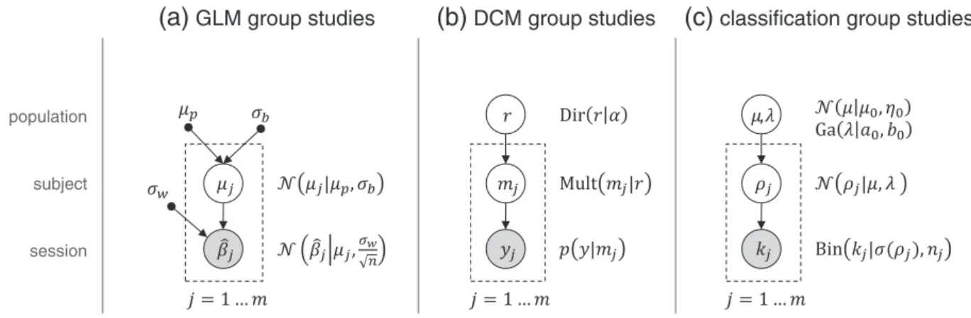
Multivariate classification algorithms have emerged from thefield of machine learning as powerful tools for predicting cognitive or patho-physiological states from neuroimaging data (Haynes and Rees, 2006). Classifiers are based on decoding models that differ in two ways from conventional mass-univariate encoding analyses based on the general linear model (GLM;Friston et al., 1995). First, multivariate approaches explicitly account for dependencies among voxels. Second, they reverse the direction of inference, predicting a contextual variable from brain activity (decoding) rather than the other way around (encoding). There are three related areas of application in which these two charac-teristics have sparked most interest.

In cognitive neuroscience, and in particular neuroimaging, classiﬁers have been employed to decode subject-speciﬁc cognitive or perceptual states from multivariate measures of brain activity, such as those obtained by fMRI (Brodersen et al., 2012b; Cox and Savoy, 2003; Haynes and Rees, 2006; Norman et al., 2006; Tong and Pratte, 2012). A second area is the

design of brain–machine interfaces which aim at decoding subjective cognitive states (e.g., intentions or decisions) from trial-wise measure-ments of neuronal activity in individual subjects (Blankertz et al., 2011; Sitaram et al., 2008). A third important domain concerns clinical applica-tions that explore the utility of multivariate decoding approaches for diagnostic purposes (Davatzikos et al., 2008; Klöppel et al., 2008, 2012; Marquand et al., 2010). Recently, decoding models have also been inte-grated with biophysical models of brain function, such as dynamic causal models (Friston et al., 2003), to afford mechanistically interpretable classi_ﬁcations (Brodersen et al., 2011a,b).

Many applications of multivariate classification operate on data with a two-level hierarchical structure. Consider, for example, a study in which a classification algorithm is used to decode from fMRI data whether a subject chose option A or B on each ofnexperimental repeti-tions or trials. This analysis gives rise tonestimated labels (representing which choice the classifier predicted on each trial) andntrue labels (indicating which option was truly chosen). Comparing predicted to true labels yields a sequence of classificationoutcomes(indicating for each trial whether the prediction was correct or incorrect). Repeating this analysis for each member of a group ofmsubjects yields the typical two-level structure (msubjects timesntrials each) that is illustrated in

Fig. 1; for a concrete example seeFigs. 7a,e. A two-level structure under-lies virtually all trial-by-trial decoding studies (see, among many others, ⁎ Corresponding author at: Translational Neuromodeling Unit (TNU), Institute for

Biomedical Engineering, University of Zurich & ETH Zurich, Wilfriedstrasse 6, CH 8032 Zurich, Switzerland.

http://dx.doi.org/10.1016/j.neuroimage.2013.03.008

Contents lists available atSciVerse ScienceDirect

NeuroImage

j o u r n a l h o m e p a g e : w w w . e l s e v i e r . c o m / l o c a t e / y n i m g

Open access under CC BY-NC-ND license.

(2)

Brodersen et al., 2012b; Chadwick et al., 2010; Harrison and Tong, 2009; Johnson et al., 2009; Krajbich et al., 2009). The same two-level structure often applies to subject-by-subject classi_ﬁcation studies (e.g., decoding a diagnostic state or predicting a clinical outcome), especially when subjects are partitioned into groups that are analyzed separately.

A hierarchical (or multilevel) design of this sort gives rise to the questions of what we can infer about the accuracy of the classifier in individual subjects, and what about the accuracy in the population from which the subjects were sampled. Any approach to answering these questions must provide a means of (i)estimation(e.g., of the accuracy itself as well as an appropriate interval that describes our uncertainty about the accuracy); and (ii)testing(e.g., whether the accuracy is signi_ficantly above chance). This paper is concerned with such subject-level and group-level inferences on classification accuracy for multilevel data.

The statistical evaluation of classi_fication performance in non-hierarchical (e.g., single-subject) applications of classification has been discussed extensively in the literature (Brodersen et al., 2010a; Langford, 2005; Lemm et al., 2011; Pereira and Botvinick, 2011; Pereira et al., 2009). By contrast, relatively little attention has thus far been de-voted to evaluating classification algorithms in hierarchical (i.e., group) settings (Goldstein, 2010; Olivetti et al., 2012). This is unfortunate since thefield would benefit from a broadly accepted standard.

Such a standard approach to evaluating classification performance in a hierarchical setting should account for two independent sources of variability:fixed-effects(i.e., within-subjects) variance that results from uncertainty about the true classification accuracy in any given subject; andrandom-effectsvariance (i.e., between-subjects variability) that reflects the distribution of true accuracies in the population from which subjects were sampled. This distinction is crucial because clas-sification outcomes obtained in different subjects cannot be treated as samples from the same distribution; in a hierarchical setting, each subject itself has been sampled from a population with an unknown intrinsic heterogeneity (Beckmann et al., 2003; Friston et al., 2005). Models that explicitly separate both sources of uncertainty are known asmixed-effectsmodels. They are the objects of interest in this paper.

Contemporary approaches to performance evaluation in classifi ca-tion group studies fall into several groups.1_{One approach rests on the} pooled sample accuracy, i.e., the number of correctly predicted trials, summed across all subjects, divided by the overall number of trials. The statistical significance of the pooled sample accuracy can be assessed using a simple classical binomial test (assuming the standard case of binary classification) that is based on the likelihood of obtaining the ob-served number of correct trials (or more) by chance (Langford, 2005). A less frequent variant of this analysis uses theaverage sample accuracy instead of the pooled sample accuracy (Clithero et al., 2011).

A second approach, more commonly used, is to consider subject-speciﬁc sample accuraciesand estimate their distribution in the popu-lation. This method typically (explicitly or implicitly) uses a classical one-tailedt-test across subjects to assess whether the population mean accuracy is greater than what would be expected by chance (e.g.,Harrison and Tong, 2009; Knops et al., 2009; Krajbich et al., 2009; Schurger et al., 2010).

In the case of single-subject studies, thefirst method (i.e., a binomial test on the pooled sample accuracy) is an appropriate approach. How-ever, there are three reasons why neither method is optimal for group studies. Firstly, both of the above methods neglect the hierarchical nature of the experiment. Thefirst method (based on the pooled sample accuracy) represents afixed-effects approach and disregards variability across subjects. This leads to overly optimistic inferences and provides results that are only representative for the specific sample of subjects studied, not for the population they were drawn from. The second meth-od (t-test on sample accuracies) does consider random effects; but it nei-ther explicitly models the uncertainty associated with subject-specific accuracies, nor does it account for violations of homoscedasticity (i.e., the differences in variance of the data between subjects).

1_{This paper focuses on}_parametric_{models for performance evaluation. While} non-parametricmethods are available (e.g., based on permutation tests), these methods can be very time-consuming in hierarchical settings and are not considered in detail here (see e.g.Hassabis et al., 2009; Just et al., 2010; Pereira and Botvinick, 2011; Pereira et al., 2009; Stelzer et al., 2013).

subject

-+

trial trial 1

subject 1 subject 2 subject

population

0

1

0

1

0

1

0

1

0

1

0

1

Fig. 1.Overview of the outcomes generated by a classification group study. In a trial-by-trial classification analysis, a classifier is trained and tested, separately for each subject, to predict a binary label (+ or−) from trial-wise correlates of brain activity. This constitutes a hierarchical design. Thefirst level concerns trial-wise classification outcomes (where 1 and 0 represent correctly and incorrectly classified trials) that are drawn from latent subject-specific classification accuracies. The second level concerns subject-specific accuracies themselves, which are drawn from a population distribution. When evaluating the performance of a classification algorithm, we are interested in inference on subject-specific accuracies and on the population accuracy itself.

(3)

The second limitation of the above methods is rooted in their distribu-tional assumptions. In the standard case of binary classification, it is rea-sonable to assume individual classi_fication outcomes to follow binomial distributions (justifying the binomial test in single-subject studies). How-ever, it is not well founded to assume that sample accuracies follow a Gaussian distribution (which, in this particular case, is the implicit as-sumption of a classicalt-test on sample accuracies). This is because a Gaussian has infinite support, which means it inevitably places probabil-ity mass on values below 0% and above 100% (for an alternative, see

Dixon, 2008).

A third problem, albeit not an intrinsic characteristic of the above methods, is their typical focus on classification accuracy, which is known to be a poor indicator of performance when classes are not perfectly balanced. Specifically, a classifier trained on an imbalanced dataset may acquire a bias in favor of the majority class, resulting in an overoptimistic accuracy. This motivates the use of an alternative performance measure, the balanced accuracy, which removes this bias from performance evaluation.

We recently proposed a solution to the three above limitations using Bayesian hierarchical models for mixed-effects inference on classiﬁ ca-tion performance. In particular, we introduced thebeta-binomialmodel and thenormal-binomialmodel for inferring on both accuracies and balanced accuracies (Brodersen et al., 2012a). Both models use a fully Bayesian framework for mixed-effects inference, are based on natural distributional assumptions, and enable more accurate inferences than the two conventional approaches described earlier. The models are inde-pendent of the type of underlying classiﬁer, which makes them widely applicable.

The practical utility of our models, however, has been limited by the high computational complexity of the underlying Markov chain Monte Carlo (MCMC) sampling algorithms required for model inver-sion (i.e., the process of passing from a prior to a posterior distribution over model parameters, given the data). MCMC is asymptotically exact; but it is also exceedingly slow, especially when performing infer-ence in a voxel-by-voxel fashion, as is common, for example, in‘ search-light’approaches (Kriegeskorte et al., 2006; Nandy and Cordes, 2003).

In this paper, we present a variational Bayes (VB) algorithm to overcome this critical limitation.2Our approach has three main fea-tures. First, we present a mixed-effects model that explicitly respects the hierarchical structure of the data. Second, the model can be equally used for inference on the accuracy and the balanced accuracy. Third, our novel variational inference scheme dramatically reduces the computa-tional complexity (i.e., runtime) compared to our previous sampling approach based on MCMC.

The paper is organized as follows. In the Theory section, we present variations of our recently developed normal-binomial model for mixed-effects inference (Brodersen et al., 2012a). These are the univariate normal-binomialmodel (for inference on theaccuracy) and the twofold normal-binomial model (for inference on the balanced accuracy).3_{We then describe a novel VB algorithm for model inversion}

and compare it to an MCMC sampler. In theApplicationssection, we provide a set of illustrative results on both synthetic data and empirical fMRI measurements. Finally, in theDiscussion, we review the key charac-teristics of our approach, compare it to similar models in other analysis domains, and discuss its role in future classiﬁcation studies.

Theory

In a hierarchical setting, a classiﬁer is typically used to predict a class label for each trial, where trials are further structured into sets,

for instance because they were recorded from different subjects. The most common situation is binary classiﬁcation, where class labels are taken from {+ 1,₋1}, denoting _‘positive_’ and _‘negative_’ trials, respectively. Less common, but equally amenable to the approach presented in this paper, are multiclass settings in which trials fall into more than two classes (seeDiscussion).

The above situation raises three principal questions (cf.Brodersen et al., 2012a). First, can one obtain successful classification at the group level? This requires statistical inference on the mean classification accura-cy in the population from which subjects were drawn. Second, do the subject-wise data permit classification in each individual? Considering each subject in isolation is statistically short-sighted, since subject-specific inference may benefit from simultaneous across-subject infer-ence (Efron and Morris, 1971). Third, which of several possible classifi ca-tion algorithms should be chosen? This is typically answered by evaluating how well an algorithm's performance generalizes (to unseen data). In a Bayesian framework, this expected performance is given by the posterior predictive density of classification performance. The present section describes a variational Bayes (VB) approach to answering these questions (Fig. 2).

The univariate normal-binomial model for inference on the accuracy Within each subject, classification outcomes can be summarized in terms of the number of correctly predicted trials,k, and the total number of trials,n. It is important to note that this summary is independent of the type of underlying classifier. This means that the model can be applied regardless of whether classification results were obtained using, for instance, logistic regression, nearest-neighbor classification, a support vector machine, or a Gaussian process classifier. Under the assumption that trial-specific predictions are conditionally independent,kfollows a binomial distribution,

p kðjπ;nÞ ¼Binðkjπ;nÞ ¼ n_k πk

1−π ð Þn−k

ð1Þ whereπrepresents the latent (unobservable) accuracy of the classiﬁer, 0≤π≤1. Thus, in a group study, where the classiﬁer has been trained and tested separately in each subject, the available data arekjandnjfor

each subjectj= 1…m.

One might be tempted to form group summariesk=∑jm= 1kjand

n=∑jm= 1njand proceed to inference onπ. However, using such a

pooled sample accuracywould assume zero between-subjects variabili-ty. In other words,πwould be treated as aﬁxed effectin the population. This approach would not permit inferences about the population; it would only allow for results to be reported as a case study (Friston et al., 1999).

Alternatively, one might summarize the data from each subject in terms of a subject-speciﬁcsample accuracy,kj/nj. One could then ask,

using a one-tailedt-test, whether sample accuracies reﬂect a normal distribution with a mean greater than what would be expected by chance (Fig. 2a). This approach no longer treats accuracy as aﬁxed effect. However, it suffers from two other problems.

First, submitting subject-specific sample accuracies to at-test as-sumes that accuracies, which are confined to the [0,1] interval, follow a normal distribution, which has infinite support. This may lead to non-interpretable results such as confidence intervals that include accuracies above 100% (or below 0%).4

Second, even if one were to overcome the above problem (e.g., using a logit transform), at-test on sample accuracies neither explicitly accounts for within-subjects uncertainty nor for violations of homoscedasticity. This is because it uses sample accuracies as summary statistics without carrying forward the uncertainty associated with them (Mumford and 2

The approach proposed in this paper has been implemented as open-source soft-ware for both MATLAB and R. The code can be downloaded from:http://www. translationalneuromodeling.org/software/.

3

Note that the terms‘univariate’and‘twofold’are used to characterize the number and structure of model parameters in each subject; these differences are unrelated to the distinction between univariate and multivariate analyses.

4

Nonparametric mixed-effects approaches make it possible to overcome this limitation; however, these are often computationally expensive and are not discussed in detail here.

(4)

Nichols, 2009). For example, sample accuracies do not distinguish be-tween an accuracy of 80% that was obtained as 80 correct out of 100 trials (i.e., an estimate with high confidence) and the same accuracy obtained as 8 out of 10 trials (i.e., an estimate with low confidence). Furthermore, no distinction regarding the confidence in the inference is being made be-tween 80 correct out of 100 trials (i.e., high confidence) and 50 correct out of 100 trials (lower confidence, since the variance of a binomial distri-bution depends on its mean and becomes maximal at a mean of 0.5).

In order to explicitly capture both within-subjects (_ﬁxed-effects) and between-subjects (random-effects) variance components, we must in-stead use a hierarchical model in which separate levels account for differ-ent sources of variability (Fig. 2b). At the level of individual subjects, for each subjectj, the number of correctly classiﬁed trialskjis modeled as

p kjjπj;nj

¼Bin kjjπj;nj

ð2Þ whereπjrepresents the latent classiﬁcation accuracy in subjectj.5Next,

at the group level, we account for variability between subjects by model-ing subject-speciﬁc accuracies as drawn from a population distribution. Thenaturalparameter of the binomial density is ln π

1−π. Thus, one possi-ble parameterization is to assume accuracies to be logit-normally distrib-uted and conditionally independent given the population parameters. In other words, each logit accuracyρj: ¼σ−

1

πj : ¼ln πj 1−πj

is drawn from a normal distribution. The inverse-sigmoid (or logit) transform σ−1

(πj) turns accuracies with support on the [0,1] interval into

log-odds with support on the real line (−∞,+∞). Thus,

p ρjjμ;λ ¼N ρjjμ;λ ¼ ffiffiffiffiffiffi λ 2π r exp −λ 2 ρj−μ 2 ð3Þ whereμ and λ represent the population mean and the population precision (i.e., inverse variance), respectively.

Since neuroimaging studies are typically conﬁned to relatively small sample sizes, an adequate expression of our prior ignorance about the population parameters is critical (cf.Woolrich et al., 2004). We use a diffuse prior onμandλsuch that the posterior will be dominated by the data (for a validation of this prior, see Applications). A

straightforward parameterization is to use independent conjugate densities: pμ μ 0;η0 ¼N μ μ 0;η0 ð4Þ pðλja0;b0Þ ¼Gaðλja0;b0Þ: ð5Þ

In the above densities,μ0andη0encode the prior mean and

pre-cision of the population mean, anda0andb0represent the shape and

scale parameter,6_{respectively, that specify the prior distribution of}

the population precision (for an alternative, seeLeonard, 1972). In summary, the univariate normal-binomial model uses a binomial distribution at the level of individual subjects and a logit-normal distribution at the group level (Fig. 2b).

In principle, inverting the above model immediately yields the desired posterior density over parameters,

pðμ;λ;ρjkÞ ¼∏ m j¼1 Bin kjjσ ρj N ρjμ;λ N μjμ0;η0 Gaðλja0;b0Þ p kð Þ : ð6Þ In practice, however, integrating the expression in the denomina-tor of the above expression, which provides the normalization constant for the posterior density, is prohibitively difﬁcult. We previ-ously described a stochastic approximation based on MCMC algo-rithms; however, the practical use of these algorithms was limited by their considerable computational complexity (Brodersen et al., 2012a). Here, we propose to invert the above model using a deter-ministic VB approximation (Fig. 2c). This approximation is no longer asymptotically exact, but it conveys considerable computational advantages. The remainder of this section describes its derivation (seeFig. 3for a summary).

Variational inference

The difficult problem offinding the exact posteriorp(μ,λ,ρ|k) can be transformed into the easier problem of_finding an approximate para-metric posteriorq(μ,λ,ρ|δ) with moments (i.e., parameters)δ. (We will omitδto simplify the notation.) Inference then reduces tofinding

5

From now on, we will omitnjunless this introduces ambiguity.

6

Under the Gamma parameterization used here, the prior expectation ofλis 〈λ〉=a0b0.

b

Bayesian mixed-effects inference (univariate normal-binomial model)

c

Variational Bayes approximation

iterative conditional optimization of posterior moments

a

Conventional

maximum-likelihood estimation

Fig. 2.Inference on classification accuracies. (a) Conventional maximum-likelihood estimation does not explicitly model within-subjects (fixed-effects) variance components and is based on an ill-justified normality assumption. It is therefore inadequate for the statistical evaluation of classification group studies. (b) The normal-binomial model respects the hierarchical structure of the study and makes natural distributional assumptions, thus enabling mixed-effects inference, which makes it suitable for group studies. The model uses the sigmoid transformσ(ρj) := (1 + exp(−ρj))−1which turns log-odds with real support (−∞,∞) into accuracies on the [0,1] interval. (b) Model inversion can be implemented efficiently using a variational Bayes approximation to the posterior densities of the model parameters (seeFig. 3for details).

(5)

a densityqthat minimizes a measure of dissimilarity betweenqandp. This can be achieved by maximizing the so-called negative free energy Fof the model, a lower-bound approximation to the log model evi-dence, with respect to (the moments of)q. For details, seeMacKay (1995), Attias (2000), Ghahramani and Beal (2001), Bishop et al. (2002), andFox and Roberts (2012). Maximizing the negative free ener-gy minimizes the Kullback–Leibler (KL) divergence between the ap-proximate and the true posterior,qandp:

KL½qjjp: ¼∭qðμ;λ;ρÞln qðμ;λ;ρÞ pðμ;λ;ρjkÞdμdλdρ ð7Þ ¼∭qðμ;λ;ρÞln qðμ;λ;ρÞ p kð;μ;λ;ρÞdμdλdρþlnp kð Þ ð8Þ ⇔lnp kð Þ ¼KL½qjjp þ lnp kð;μ;λ;ρÞ qðμ;λ;ρÞ qðμ;λ;ρÞ |fflfflfflfflfflfflfflfflfflfflfflfflfflfflfflfflfflfflfflfflffl{zfflfflfflfflfflfflfflfflfflfflfflfflfflfflfflfflfflfflfflfflffl} ¼:F qð;kÞ : ð9Þ

This means that the log-model evidence lnp(k) can be expressed as the sum of (i) the KL-divergence between the approximate and the true posterior and (ii) the negative free energyF(q,k). Because the KL-divergence cannot be negative, maximizing the negative free en-ergy with respect toqminimizes the KL-divergence and thus results in an approximate posterior that is maximally similar to the true pos-terior. At the same time, maximizing the negative free energy pro-vides a lower-bound approximation to the log-model evidence, which permits Bayesian model comparison (Bishop, 2007; Penny et al., 2004). In summary, maximizing the negative free energyF(q,k) in Eq.(9)enables both inference on the posterior density over param-eters and model comparison. In this paper, we are primarily interest-ed in the posterior density.

In trying to maximizeF(q,k), variational calculus tells us that

∂F qð ;kÞ

∂q ¼0⇒qðμ;λ;ρÞ∝exp½ |fflfflfflfflfflfflfflfflfflfflffl{zfflfflfflfflfflfflfflfflfflfflffl}lnp kð ;μ;λ;ρÞ negative variational energy

ð10Þ

This means that the approximate posterior which maximizes the negative free energy is equal to the true posterior and thus propor-tional to the joint density over data and parameters7_{(with the}

nor-malization constant being given by the model evidence). In other words, the VB approach is complete in the sense that, in the absence of any other approximations, optimizingFwith respect toqyields the exact posterior density and model evidence.

Mean-ﬁeld approximation

To make the optimization on the l.h.s. in Eq.(10)tractable, we as-sume that the joint posterior over all model parameters factorizes into speciﬁc parts. Using one density for each variable,

qðμ;λ;ρÞ ¼qð Þμ qð Þλqð Þρ ð11Þ the mean-ﬁeld assumption turns the problem of maximizingF(q,k) into the problem of deriving three expectations:

I1ð Þ ¼μ hlnp kð;μ;λ;ρÞiqðλ;ρÞ ð12Þ

I2ð Þ ¼λ hlnp kð;μ;λ;ρÞiqðμ;ρÞ ð13Þ

I3ð Þ ¼ρ hlnp kð;μ;λ;ρÞiqðμ;λÞ: ð14Þ

This transformation has several advantages over working with Eq.

(10)directly: it makes it more likely that we canﬁnd the exact distri-butional form of a marginal approximate posterior (as will be the case forμandλ); it may make the Laplace assumption more appropriate in those cases where we cannot identify aﬁxed form (as will be the case for_ρ); and it often provides us with interpretable update equations (as will be the case, in particular, forμandλ).

Parametric assumptions

Due to the structure of the model, the posteriors on the population parametersμandλare conditionally independent given the data. In addition, owing to the conjugacy of their priors, the posteriors onμ andλfollow the same distributions and do not require any additional parametric assumptions:

q_{ð Þ ¼}_μ N_μ_j_μ_μ_;_η_μ _ð15_Þ

qð Þ ¼λ Gaðλja_λ;b_λÞ: ð16Þ

Subject-speci_ﬁc (logit) accuracies q_≡(_ρ1,…,ρm) are also

condi-tionally independent given the data. This is a consequence of the fact that the posterior for each subject only depends on its Markov blanket, i.e., the subject's data and the population parameters (but not the other subject's logit accuracies). This can be seen from the fact that

qðμ;λ;ρÞ ¼qð Þμ qð Þλ qð Þρ ð17Þ ¼qð Þμqð Þ∏λ m

j¼1q ρj : ð18Þ

However, we do require a distributional assumption for the above subject-speciﬁc posteriors to make model inversion feasible. Here, we assume posterior subject-speciﬁc (logit) accuracies to be normally distributed:

qð Þ ¼ρ ∏m

j¼1N ρjjμμj;ηρj

: ð19Þ

The conditional independence in Eq.(19)differs in a subtle but important way from the assumption ofunconditionalindependence that is implicit in random-effects analyses on the basis of at-test on subject-speciﬁc sample accuracies (seeIntroduction). In the case of such t-tests, estimation in each subject only ever uses data from that same subject. By contrast, the subject-speci_ﬁc posteriors in Eq.

(20)borrow strength fromallobservations. This can be seen from the fact that the subject-speciﬁc posteriorsq(ρ) are computed with respect to the population posteriorsq(_μ) andq(_λ) which are them-selves informed by observations from the entire group (see Eqs.(12)–(14)).

Derivation of variational densities

For each mean-ﬁeld part in Eq.(11), the variational densityq(⋅) can be obtained by evaluating the variational energyI(⋅), as described next. Theﬁrst variational energy concerns the posterior density over the population meanμ. It is given by

I1ð Þ ¼μ hlnp kð;μ;λ;ρÞiqðλ;ρÞ ð20Þ ¼_hlnp k_ð _j_ρ_Þ_i_q_ð_λ_;_ρ_Þ_þ_hlnp_ð_ρ_j_μ_;_λ_Þ_i_q_ð_λ_;_ρ_Þ_þ_hlnp_ð_μ_;_λ_Þ_i_q_ð_λ_;_ρ_Þ _ð21_Þ ¼∑m j¼1 lnN ρjjμ;λ D E qðλ;ρÞ þ lnN μjμ0;η0 Gaðλja0;b0Þ qðλ;ρÞþc ð22Þ 7

The dependence of the joint probability in Eq.(10)on the prior (μ0,η0,a0,b0) has been omitted for brevity.

(6)

¼∑m j¼1 1₂lnλ−₂1ln 2π−λ₂ ρj−μ 2 qðλ;ρÞ þ 1₂lnη0−η₂0ðμ−μ0Þ 2 D E qðλ;ρÞþc ð23Þ ¼∑m j¼1−1₂ λ ρ 2 j−2λρjμþλμ 2 D E qðλ;ρÞ− η0 2ðμ−μ0Þ 2 þc _ð24_Þ ¼−1₂∑m j¼1 −2μμρjþμ 2 h i a_λb_λþμ η0 μ0− 1 2μ þc ð25Þ ¼μa_λb_λ ₋1 2mμþ∑ m j¼1μρj þμ η0 μ0− 1 2μ þc _ð26_Þ

where the symbolcis used for any expression that is constant with respect toμ.

In principle, we could proceed by optimizing the sufﬁcient statis-tics of the approximate posterior. Instead, we only optimize the mean and equate the variance to theobserved information, i.e., the negative curvature at the mode. This procedure is known as the La-place approximation(or normal approximation) and implies that the negative free energy is a function simply of the posterior means (as opposed to a function of the posterior means and covariances). It is a local, rather than a global, optimization solution.

Conveniently, the Laplace approximation is typically more accu-rate for the conditional posterior (of one parameter given the others) than for the full posterior (of all parameters). In addition, it is compu-tationally efﬁcient (seeDiscussion) and often gives rise to interpret-able update equations (see below).

Setting theﬁrst derivative to zero yields an analytical expression for the maximum,

dI1ð Þμ dμ ¼−μ η0þmaλbλ þμ0η0þaλbλ∑ m j¼1μρj¼0 ð27Þ ⇒μ¼μ0η0þaλbλ∑ m j¼1μρj η0þmaλbλ : ð28Þ

Having found the mode of the approximate posterior, we can use a second-order Taylor expansion to obtain closed-form approximations for its moments:

μμ¼μ and ð29Þ ημ¼− dI21ð Þμ dμ2 _μ_¼_μ¼η0þmaλbλ: ð30Þ

Thus, the posterior density of the population mean logit accuracy under our mean-ﬁeld and Gaussian approximations isN(μ|μμ,ημ).

The use of a Laplace approximation, as we do here, often leads to in-terpretable update equations. In Eq.(30), for example, we can see that the posterior precision of the population mean (ημ) is simply the sum of the prior precision (η0) and the mean of the posterior population

pre-cision (aλbλ), correctly weighted by the number of subjectsm. Based on the above approximation for the posterior logit accuracy, we can see that the posterior mean accuracy itself,ξ : =σ(μ), is logit-normally distributed and can be expressed in closed form,

logitN ξjμμ;ημ ¼_ξ_ð₁1₋_ξ_Þ ffiffiffiffiffiffi ημ 2π r exp −η₂μ σ−1 ξ ð Þ−μμ 2 ð31Þ

conditional maximization until convergence

(negative) free energy

Newton-Raphson

variational algorithm with Laplace approximations parametric assumptions

mean-field approximation variational inference

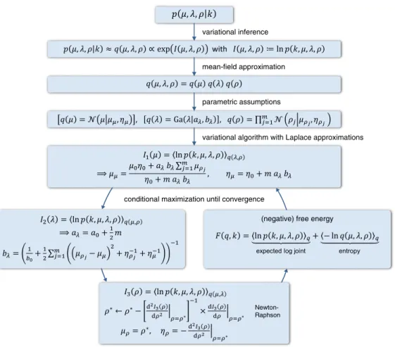
Fig. 3.Variational inversion of the univariate normal-binomial model. This schematic summarizes the individual steps involved in the variational approach to the inversion of the univariate normal-binomial model, as described in the main text (seeTheory).

(7)

whereμμandημrepresent the posterior mean and precision, respec-tively, of the population mean logit accuracy.

The second variational energy concerns the population precision_λ and is given by I2ð Þ ¼λ hlnp kð ;μ;λ;ρÞiqðμ;ρÞ ð32Þ ¼m₂lnλ−λ₂∑m j¼1 μρj−μμ 2 þη−1 ρj þη− 1 μ þða0−1Þlnλ−_bλ 0þ c ð33Þ wherecrepresents a term that is constant with respect to λ. The above expression already has the form of a log-Gamma distribution with parameters a_λ¼a0þ 1 2m and ð34Þ b_λ¼ _b1 0þ 1 2∑ m j¼1 μρj−μμ 2 þη−1 ρj þη− 1 μ ₋1 : ð35Þ

From this we can see that the shape parameteraλis a weighted sum of prior shapea0and datam. When viewing the second parameter as a ‘rate’coefficientbλ−1(as opposed to a shape coefficientbλ), it becomes clear that the posterior rate really is a weighted sum of: the prior rate (b0−1); the dispersion of subject-specific means; their variances (η−ρj1);

and our uncertainty about the population mean (ημ−1).

The variational energy of the third partition concerns the model parameters representing subject-speci_ﬁc latent accuracies. This ener-gy is given by I3ð Þ ¼ρ hlnp kð ;μ;λ;ρÞiqðμ;λÞ ð36Þ ¼∑m j¼1 kjlnσ ρj þ nj−kj ln 1−σ ρj −1₂a_λb_λ ρj−μμ 2 þc: ð37Þ Since an analytical expression for the maximum of this energy does not exist, we resort to an iterative Newton–Raphson scheme based on a quadratic Taylor-series approximation to the variational energyI3(ρ). For this, we begin by considering the Jacobian

dI3ð Þρ dρ j ¼∂I3ð Þρ ∂ρj ¼ kj−njσ ρj þaλbλ μμ−ρ ð38Þ and the Hessian

d2I3ð Þρ dρ2 ! jk ¼∂ 2 I3ð Þρ ∂ρj∂ρk ¼−δjk njσ ρj 1−σ ρj þa_λb_λ ð39Þ where the Kronecker delta operatorδjkis 1 ifj=kand 0 otherwise.

As noted before, the absence of off-diagonal elements in the Hessian is not based on an assumption of conditional independence of subject-speciﬁc posteriors; it is a consequence of the mean-ﬁeld sep-aration in Eq.(11). Each GN iteration performs the update

ρ←ρ− d 2 I3ð Þρ dρ2 _ρ_¼_ρ 2 4 3 5 −1 dI3ð Þρ dρ _ρ_¼_ρ ð40Þ

until the vectorρ*_{converges, i.e.,}_‖_ρ⁎

current−ρ⁎previous‖2b10−3. Using

this maximum, we can use a second-order Taylor expansion (i.e., the La-place approximation) to set the moments of the approximate posterior:

μρ¼ρ and ð41Þ ηρ¼− d2I3ð Þρ dρ2 _ρ_¼_ρ : ð42Þ

Variational algorithm and free energy

The expressions for the three variational energies depend on one another. This circularity can be resolved by iterating over the expres-sions sequentially and updating the moments of each approximate marginal given the current moments of the other marginals. This ap-proach of conditional maximization (or stepwise ascent) maximizes the (negative) free energyF≡F(q,k) and leads to approximate mar-ginals that are maximally similar to the exact marmar-ginals.

The free energy itself can be expressed as the sum of the expected log-joint density (over the data and the model parameters) and the Shannon entropy of the approximate posterior:

F¼hlnp kð;μ;λ;ρÞiq |fflfflfflfflfflfflfflfflfflfflfflfflfflffl{zfflfflfflfflfflfflfflfflfflfflfflfflfflffl} expected log joint

þh−lnqðμ;λ;ρÞiq |fflfflfflfflfflfflfflfflfflfflfflfflfflffl{zfflfflfflfflfflfflfflfflfflfflfflfflfflffl}

entropyH q½

: ð43Þ

We begin by considering the expectation of the log joint w.r.t. the variational posterior: lnp kð;μ;λ;ρÞ h iq¼∑m j¼1 ln Bin kjjσ ρj þlnNρjjμ;λ D E qð Þμ qð Þλ |fflfflfflfflfflfflfflfflfflfflfflfflfflfflfflfflfflfflfflfflfflfflfflfflfflfflfflfflfflfflfflfflfflfflfflfflfflfflfflfflfflfflfflfflffl{zfflfflfflfflfflfflfflfflfflfflfflfflfflfflfflfflfflfflfflfflfflfflfflfflfflfflfflfflfflfflfflfflfflfflfflfflfflfflfflfflfflfflfflfflffl} ≡Ið Þρj * + qð Þρj þ lnNμjμ0;η0 qþhln Gaðλja0;b0Þiq: ð44Þ The above expression contains the variational energy ofρj,

I ρj ¼ ln Bin kjjσ ρj þ1₂ðψð Þ þa_λ lnb_λÞ −1₂ln 2π−1₂a_λb_λ ρj−μμ 2 þη−1 μ _ð45Þ

whereψ(⋅) is the digamma function.I(ρj) is the only term in Eq.(44)

whose expectation [w.r.t.q(ρj)] cannot be derived analytically. Under

the Laplace approximation, however, it is replaced by a second-order Taylor expansion around the variational posterior modeμρj,

I ρj ≈I μρj þI′ μρj ρj−μρj

þ1₂I″ μρj ρj−μρj

2

: ð46Þ

This allows us to approximate the expectation ofI(ρj) by

I ρj D E q_{ð Þ}ρj ≈ I μρj D E q_{ð Þ}ρj |fflfflfflfflfflfflfflfflfflffl{zfflfflfflfflfflfflfflfflfflffl} I μρ_j þI′ μρj ρj−μρj D E q_{ð Þ}ρj |fflfflfflfflfflfflfflfflfflfflffl{zfflfflfflfflfflfflfflfflfflfflffl} 0 þ1 2I ″ _μ ρj |fflfflfflffl{zfflfflfflffl} −ηρ_j ρj−μρj 2 qð Þρj |fflfflfflfflfflfflfflfflfflfflfflfflfflfflffl{zfflfflfflfflfflfflfflfflfflfflfflfflfflfflffl} η−1 ρj ð47Þ ¼I μρj − 1 2 ð48Þ

where the equality I″ μρj ¼−ηρj follows directly from Eq.(42).

Hence, the expected log joint is:

lnp kð ;μ;λ;ρÞ h iq≈ 1 2ln η0 2_π− η0 2 μμ−μ0 2 þη−1 μ zfflfflfflfflfflfflfflfflfflfflfflfflfflfflfflfflfflfflfflfflfflfflfflfflfflfflfflfflfflfflffl}|fflfflfflfflfflfflfflfflfflfflfflfflfflfflfflfflfflfflfflfflfflfflfflfflfflfflfflfflfflfflffl{hln Nðμjμ0;η0Þiq −ln_Γ_{ð Þ−}a₀ a₀lnb₀_þ_ða₀₋1_Þ_ð_ψ_{ð Þ þ}a_λ lnb_λ_Þ−aλbλ b₀ zfflfflfflfflfflfflfflfflfflfflfflfflfflfflfflfflfflfflfflfflfflfflfflfflfflfflfflfflfflfflfflfflfflfflfflfflfflfflfflfflfflfflfflfflfflfflfflfflfflfflfflffl}|fflfflfflfflfflfflfflfflfflfflfflfflfflfflfflfflfflfflfflfflfflfflfflfflfflfflfflfflfflfflfflfflfflfflfflfflfflfflfflfflfflfflfflfflfflfflfflfflfflfflfflffl{hlnGaðλja0;b0Þiq þX m j¼1 ln Bin kjjσ μρj þ1₂_ðψ_{ð Þ þ}a_λ lnb_λ_Þ−1 2ln 2π −1₂a_λb_λ μρj−μμ 2 þη−1 μ −1₂ ð49Þ

(8)

The second term of the free energy in Eq.(43)is the entropyH[q] of the variational posterior:

−lnqðμ;λ;ρÞ h iq¼ 1 2ln 2πe ημ zfflfflfflfflffl}|fflfflfflfflffl{ H N½ ðμjμμ;ημÞ þX m j¼1 1 2ln 2πe ηρj zfflfflfflfflffl}|fflfflfflfflffl{ H N ρjjμρj;ηρj h i þazfflfflfflfflfflfflfflfflfflfflfflfflfflfflfflfflfflfflfflfflfflfflfflfflfflfflfflfflfflfflfflfflfflffl}|fflfflfflfflfflfflfflfflfflfflfflfflfflfflfflfflfflfflfflfflfflfflfflfflfflfflfflfflfflfflfflfflfflffl{_λþlnb_λþlnΓð Þ þa_λ ð1−a_λÞψð Þa_λ H½Gaðλja_λ;b_λÞ ð50Þ

Substituting Eqs.(49) and (50)into Eq.(43)yields an expression for the free energy,

F≈ 1₂lnη0 ημ− η0 2 μμ−μ0 2 þη−1 μ þa_λ−a0lnb0þlnΓ a_λ ð Þ Γð Þa0 −a_λb_λ 1 b0þ m 2ημ ! þ a0þ m 2 lnb_λþ a0−aλþ m 2 ψð Þa_λ þ1₂þX m j¼1 ln Bin kjσ μρj −₂1a_λb_λ_μ_ρj₋_μ_μ2₋1 2lnηρj : ð51Þ The availability of the above approximation to the free energy leads to a straightforward variational algorithm. The algorithm is ini-tialized by setting the moments of all approximate posteriors to the moments of their respective priors. It terminates when

Fcurrent−Fpreviousb10− 3

ð52_Þ i.e., when the free energy has converged. This criterion typically leads to the same inference as a criterion based on the parameter estimates themselves, e.g., θcurrent−θprevious 2b10−3 _ð53_Þ where convergence of θ≡ μμ;ημ;aλ;bλ;μρ1;…;μρm;ηρ1;…;ηρm is expressed through a bound on their (squared) ‘2-norm. However,

computing (an approximation to) the free energy itself has the addi-tional advantage that it provides an approximation to the log model evidence (see Eqs.(9) and (43)), which permits Bayesian model se-lection (for an example, seeBrodersen et al., 2012a).

MCMC sampling

The variational Bayes scheme presented above is computationally highly efficient; it typically converges after just a few iterations. How-ever, its results are only exact to the extent to which its distributional assumptions are justified. To validate these assumptions, we com-pared VB to an asymptotically exact stochastic approach, i.e., Markov chain Monte Carlo (MCMC), which is computationally much more ex-pensive than variational Bayes but exact in the limit of infinite runtime. In the Supplemental Material, we describe a Gibbs sampler for inverting the univariate normal-binomial model introduced above. This algorithm is analogous to the one we previously introduced for the inversion of the bivariate normal-binomial model inBrodersen et al. (2012a). It proceeds by cycling over model parameters, drawing sam-ples from their full-conditional distributions, until the desired number of samples (e.g., 106) has been generated (see Supplemental Material). Unlike VB, which was based on a mean-field assumption, the posteri-or obtained through MCMC retains any potential conditional dependen-cies among the model parameters. The algorithm is computationally burdensome; but it can be used to validate the distributional assumptions underlying variational Bayes (seeApplications).

The twofold normal-binomial model for inference on the balanced accuracy

Seemingly strong classification accuracies can be trivially obtained on datasets consisting of different numbers of representatives from either class. For instance, a classifier might assign every example to the majority class and thus achieve an accuracy equal to the propor-tion of test cases belonging to the majority class. Thus, the use of clas-sification accuracy as a performance measure may easily lead to optimistic inferences (Akbani et al., 2004; Brodersen et al., 2010a, 2012a; Chawla et al., 2002; Japkowicz and Stephen, 2002).

This has motivated the use of a different performance measure: the balanced accuracy, deﬁned as the arithmetic mean of sensitivity and speciﬁcity, or the average accuracy obtained on either class,

φ: ¼1₂πþþπ− ð54Þ

whereπ+_{: =}_σ₍_μ+_{) and}_π−_{: =}_σ₍_μ−_{) denote the (population)}

classi-fication accuracies on positive and negative trials, respectively.8The bal-anced accuracy reduces to the conventional accuracy whenever the classifier performed equally well on either class; and it drops to chance when the classifier performed well purely because it exploited an existing class imbalance. We will revisit the conceptual differences be-tween accuracies and balanced accuracies in theDiscussion. In this sec-tion, we show how the univariate normal-binomial model presented above can be easily extended to allow for inference on the balanced accuracy.

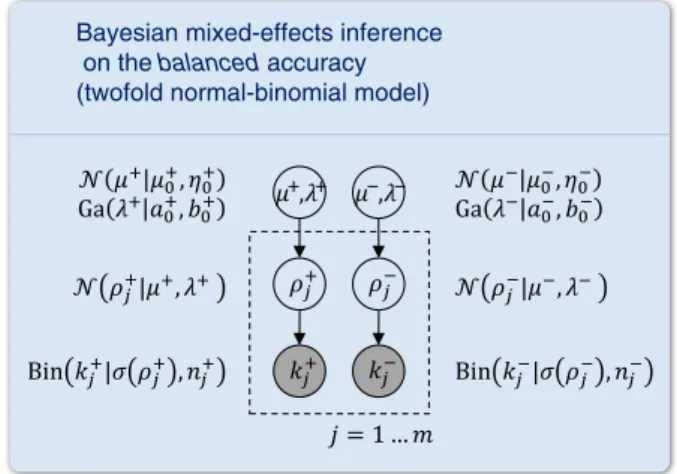
We have previously explored different ways of constructing models for inference on the balanced accuracy (Brodersen et al., 2012a). Here, we infer on the balanced accuracy by duplicating our generative model for accuracies and applying it separately to data from the two classes. This constitutes thetwofoldnormal-binomial model (Fig. 4).

To infer on the balanced accuracy, we separately consider the number of correctly classiﬁed positive trialskj+and the number of

correctly predicted negative trialskj−for each subjectj= 1…m. We

next describe the true accuracies within each subject asπj+andπj−.

The population parametersμ+_,_λ+_and_μ−_,_λ−_{then represent the}

population accuracies on positive and negative trials, respectively. Inverting the model proceeds by inverting its two parts indepen-dently. However, in contrast to the inversion of the univariate

Bayesian mixed-effects inference on the balanced accuracy (twofold normal-binomial model)

Fig. 4.Inference on balanced accuracies. The univariate normal-binomial model (Fig. 2) can be easily extended to enable inference on the balanced accuracy. Speciﬁcally, the model is inverted separately for classiﬁcation outcomes obtained on positive and neg-ative trials. The resulting posteriors are then recombined (see main text).

8

(9)

normal-binomial model, we are no longer interested in the posterior densities over the population mean accuraciesμ+_and_μ−_themselves.

Rather, we wish to obtain the posterior density of the balanced accura-cy, pϕjkþ;k−¼p 1 2 σ μ þ _þ_{σ μ}_ð −_Þ kþ;k− : ð55Þ Unlike the population mean accuracy (Eq. (29)), which was logit-normally distributed, the posterior mean of the populationbalanced accuracy can no longer be expressed in closed form. The same applies to subject-speciﬁc posterior balanced accuracies. We therefore approxi-mate the respective integrals by (one-dimensional) numerical integra-tion. If we were interested in the sum of the two class-speciﬁc accuracies,s: =σ(μ+_{) +}_σ₍_μ−_{), we would consider the convolution}

of the distributions forσ(μ+

) andσ(μ−_), p s k þ;k−¼∫s 0pσ μ_{ð Þ}þ s−z k þ p_{σ μ}_ð−_Þðz kj Þ−dz ð56Þ wherep_{σ μ}_{ð Þ}þ andp_{σ μ}_ð−_Þrepresent the individual posterior distributions of

the population accuracy on positive and negative trials, respectively. In the same spirit, the modiﬁed convolution

pϕjkþ;k−¼∫2φ

0 pσ μ_{ð Þ}þ 2ϕ−zjkþ

p_{σ μ}_ð−_Þðz kj Þ−dz ð57Þ

yields the posterior distribution of the arithmetic mean of two class-speci_ﬁc accuracies, i.e., the balanced accuracy.

Applications

This section illustrates the sort of inferences that can be made using VB in a classification study of a group of subjects. We begin by consider-ing synthetic classification outcomes to evaluate the consistency of our approach and illustrate its link to classicalfixed-effects and random-effects analyses. We then apply our approach to empirical fMRI data obtained from a trial-by-trial classification analysis.

Application to synthetic data

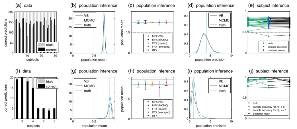
We examined the statistical properties of our approach in two typical settings: (i) a larger simulated group of subjects with many trials each; and (ii) a small group of subjects with few trials each, including missing trials. Before we turn to the results of these simula-tions, we will pick one simulated dataset from either setting to illustrate inferences supported by our model (Fig. 5).

Theﬁrst synthetic setting is based on a group of 30 subjects with 200 trials each (i.e., 100 trials in each class). Outcomes were generated using the univariate normal-binomial model with a population mean (logit accuracy) ofμ= 1.1 (corresponding to a population mean accu-racy of 71%) and a relatively high logit population precision ofλ= 4 (corresponding to a population accuracy standard deviation of 9.3%;

Fig. 5a). MCMC results were based on 100,000 samples, obtained from 8 parallel chains (see Supplemental Material).

In inverting the model, the parameter of primary interest isμ, the (logit) population mean accuracy. Our simulation showed a typical result in which the posterior distribution of the population mean was sharply peaked around the true value, with its shape virtually indistin-guishable from the corresponding MCMC result (Fig. 5b). In practice, a good way of summarizing the posterior is to report a central 95% pos-terior probability interval (or Bayesian credible interval). Although this interval is conceptually different from a classical (frequentist) 95% confidence interval, in this particular case the two intervals agreed very closely (Fig. 5c), which is typical in the context of a large sample size. In contrast, fixed-effects intervals were overconfident when

based on the pooled sample accuracy and underconﬁdent when based on the average sample accuracy (Fig. 5c).

Another informative way of summarizing the posterior population mean is to report the posterior probability masspthat is below chance (e.g., 0.5 for binary classification). We refer to this probability as the (posterior)infraliminal probabilityof the classi_fier (cf.Brodersen et al., 2012a). Compared with a classicalp-value, it has a deceptively similar, but more natural, interpretation. Rather than representing the frequency of observing the observed outcome (or a more extreme outcome) under the‘null’hypothesis of a classifier operating at or below chance (classical p-value), the infraliminal probability represents our posterior belief that the classifier does not perform better than chance. In the above simula-tion, we obtainedp≈10−10_.

We next considered the truesubject-speciﬁcaccuracies and compared them (i) with conventional sample accuracies and (ii) with VB posterior means (Fig. 5e). This comparison highlighted one of the principal features of hierarchical models, that is, theirshrinkageeffect. Because of the limited numbers of trials, sample accuracies exhibited a larger vari-ance than ground truth; accordingly, the posterior means, which were informed by data from the entire group, appropriately compensated for this effect by shrinking to the group mean. This effect is also known as regression to the meanand dates back to works as early as Galton's law of‘regression towards mediocrity’(Galton, 1886). It is obtained naturally in a hierarchical model and, as we will see below, leads to systematically more accurate posterior inferences at the single-subject level.

We repeated the above analysis on a sample dataset from a second simulation setting. This setting was designed to represent the exam-ple of a small group with varying numbers of trials across subjects.9

Such a scenario is important to consider because it occurs in real-world applications whenever the number of trials eligible for subse-quent classiﬁcation is not entirely under experimental control. Vary-ing numbers of trials also occur, for example, in clinical diagnostics of diseases like epilepsy where one may have different numbers of observations per patient. Classiﬁcation outcomes were generated using the univariate normal-binomial model with a population mean logit accuracy ofμ= 2.2 and a low logit population precision of λ= 1; the corresponding population mean accuracy was 87%, with a population standard deviation of 11.2% (Fig. 5f).

Comparing the resulting posteriors (Figs. 5g–j) to those obtained on theﬁrst dataset, several differences are worth noting. Concerning the population parameters (Figs. 5g,i), all estimates remained in close agreement with ground truth; at the same time, minor discrep-ancies began to arise between variational and MCMC approximations, with the variational results slightly too precise (Figs. 5g,i). This can be seen best from the credible intervals (Fig. 5h, black). By comparison, an example of inappropriate inference can be seen in the frequentist conﬁdence interval for the population accuracy, which does not only exhibit an optimistic shift towards higher performance but also includes accuracies above 100% (Fig. 5h, red).

Another typical consequence of a small dataset with variable trial numbers can be seen in the shrinkage of subject-specific inferences (Fig. 5j). In comparison to thefirst setting, there are fewer trials per subject, and so the shrinkage effect is stronger. In addition, subjects with fewer trials (red) are shrunk more than those with more trials (blue). Thus, the order between sample accuracies and posterior means has changed, as indicated by crossing black lines. Restoring the correct order of subjects can become important, for example, when one wishes to relate subject-specific accuracies to independent subject-specific characteristics, such as behavioral, demographic, or genetic information.

The primary advantage of VB over sampling algorithms is its compu-tational efﬁciency. To illustrate this, we examined the computational load required to invert the normal-binomial model on the dataset

9

Note that the heteroscedasticity in this dataset results both from the fact that sub-jects have different numbers of trials and from their different sample accuracies.

(10)

10 20 30 0 50 100 150 200 subjects correct predictions

(a)

data

trials correct 0 0.5 1 0 5 10 15 20 population mean

(b)

population inference

VB MCMC truth 0 0.5 1

(c)

population inference

population mean MFX (VB) MFX (MCMC) FFX (pooled) FFX (averaged) RFX 0 5 10 0 0.2 0.4 0.6 0.8 population precision

(d)

population inference

(e)

subject inference

truth sample accuracy posterior mean 2 4 6 8 0 5 10 15 20 subjects correct predictions

(f)

data

trials correct 0 0.5 1 0 5 10 15 20 population mean

(g)

population inference

(h)

population inference

population mean MFX (VB) MFX (MCMC) FFX (pooled) FFX (averaged) RFX 0 5 10 0 0.2 0.4 0.6 0.8 population precision

(i)

population inference

(j)

subject inference

truth

sample accuracy for n(j) > 5 sample accuracy for n(j) <= 5 posterior mean

Fig. 5.Application to simulated data. Two simple synthetic datasets illustrate the sort of inferences that can be obtained using a mixed-effects model. (a) Simulated data, showing the number of trials in each subject (gray) and the number of correct predictions (black). (b) Resulting posterior density of the population mean accuracy when using variational Bayes or MCMC. (c) Posterior densities can be summarized in terms of central 95% posterior intervals. Here, the two Bayesian intervals (blue/black) are compared with a frequentist random-effects 95% confidence interval and withfixed-effects intervals based on the pooled and the averaged sample accuracy. (d) Posterior densities of the population precision (inverse var-iance). (e) The benefits of a mixed-effects approach in subject-specific inference can be visualized (cf.Brodersen et al., 2012a) by contrasting the increase in dispersion (as we move from ground truth to sample accuracies) with the corresponding decrease in dispersion (as we move from sample accuracies to posterior means). This effect is a consequence of the hierarchical structure of the model, and it yields better estimates of ground truth (cf.Figs. 7d,h). Notably, shrinking may change the order of subjects (when sorted by accuracy) since its extent depends on the subject-specific (first-level) posterior uncertainty. Note that the x-axis does not represent any quantity by itself but simply serves to space out the three groups of data points (ground truth, samples accuracies, and posterior means). Overlapping sample accuracies are additionally scattered horizontally for better visibility. (f–j) Same plots as in the top row, but based on a different simulation setting with a much smaller number of subjects and a smaller and more heterogeneous number of trials in each subject. The smaller size of the dataset enhances the merits of mixed-effects inference over conventional approaches and increases the shrinkage effect in subject-specific accuracies. K.H. Brodersen et al. / NeuroImage 76 (2013) 345 – 361

(11)

shown inFig. 5a. Rather than measuring computation time (which is platform-dependent), we considered the number of ﬂoating-point operations (FLOPs), which we related to the absolute error of the in-ferred posterior mean of the mean population accuracy (in percentage points;Fig. 6). We found that MCMC used 4000 times more arithmetic operations to achieve an estimate that was better than VB by no more than 0.13 percentage points.

Application to a larger number of simulations

Moving beyond the single case examined above, we replicated our analysis many times while varying the true population mean accuracy between 0.5 and 0.9. For each point, we ran 200 simulations. This allowed us to examine the properties of our approach from a frequentist perspective (Fig. 7).

In theﬁrst setting (Fig. 7, top row), each simulation was based on synthetic classiﬁcation outcomes from 30 subjects with 200 trials each, as described in the previous section. One instance of these simulations is shown as an example (Fig. 7a); all subsequent plots are based on 200 independent datasets generated in the same way.

We began by asking, in each simulation, whether the population mean accuracy was above chance (0.5). We answered this question by computingp-values using the followingfive methods: (i)fixed-effects inference based on a binomial test on the pooled sample accuracy (orange); (ii)fixed-effects inference based on a binomial test on the average sample accuracy (violet); (iii) mixed-effects inference using VB (solid black); (iv) mixed-effects inference using an MCMC sampler with 100,000 samples (dotted black); and (v) random-effects inference using at-test on subject-specific sample accuracies (red).

An important aspect of inferential conclusions (whether frequentist or Bayesian under a diffuse prior) is their validity with respect to a given test size. For example, when using a test size ofα= 0.05, we expect the test statistic to be at or beyond the corresponding critical value for the‘null’ hypothesis (of the classiﬁcation accuracy to be at or below the level of chance) in precisely 5% of all simulations. We thus plotted the empiricalspeciﬁcity, i.e., the fraction of false rejections, as a function of test size (Fig. 7b). For any method to be a valid test, p-values should be uniformly distributed on the [0, 1] interval under the‘null’; thus, the empirical cumulative distribution function should approximate the main diagonal.

105 ₁₀6 ₁₀7 ₁₀8 ₁₀9

10-2 100 102

FLOPs

absolute error (% points)

MCMC VB

0.01 s _{4:18 min}

Fig. 6.Estimation error and computational complexity. VB and MCMC differ in the way es-timation error and computational complexity are traded off. The plot shows eses-timation error in terms of the absolute difference of the posterior mean of the population mean ac-curacy in percentage points (y-axis). Computational complexity is shown in terms of the number ofﬂoating point operations (FLOPs) consumed. VB converged after 370,000 FLOPs (iterative updateb10−6_{) to a posterior mean of the population mean accuracy of} 73.5%. Given a true population mean of 73.9%, the estimation error of VB was−0.4 per-centage points. In contrast, MCMC used up 1.47 × 109

FLOPs to draw 10,000 samples (excluding 100 burn-in samples). Its posterior mean estimate was 73.6%, implying an error of−0.26 percentage points. Thus, while MCMC ultimately achieved a marginally lower error, VB was computationally more efﬁcient by more than 3 orders of magnitude. It should be noted that the plot uses log–log axes for readability; the difference between the two algorithms would be visually even more striking on a linear scale.

(a)

example data

trials correct 0 0.5 1 0 0.2 0.4 0.6 0.8 1 p(reject | π = 0.5; α ) test size α

(b)

specificity

0.5 0.75 1 0 0.2 0.4 0.6 0.8 1

population mean accuracy

p(reject | π )

(c)

sensitivity at

α

= 0.05

MFX (VB) MFX (MCMC) FFX (pooled) FFX (averaged) RFX (t-test) 0.5 0.75 2 2.5 3 3.5

RMSE (% points)

(d)

risk

VB MCMC sample accuracy 2 4 6 8 0 5 10 15 20 subjects correct predictions

(e)

example data

trials correct 0 0.5 1 0 0.2 0.4 0.6 0.8 1 p(reject | π = 0.5; α ) test size a

(f)

specificity

0.5 0.75 1 0 0.2 0.4 0.6 0.8 1

p(reject | π )

(g)

sensitivity at

α

= 0.05

0.5 0.75 8 10 12 14 16

RMSE (% points)

(h)

risk

Fig. 7.Application to a larger number of simulations. (a) One example of 200 simulations of synthetic classification outcomes (generated using the same model as inFig. 5a). (b) Specificity of competing methods for testing whether the population mean accuracy is greater than chance, given a true population mean of 0.5. (c) Power curve, testing whether the population mean accuracy is greater than chance, given different true population mean accuracies. (d) Comparison of accuracy of subject-specific estimates, using different inference methods. (e) Example of a smaller dataset (sampled from the same model as inFig. 5f). (f–h) Same analyses as above, but based on smaller experiments.

(12)

As can be seen fromFig. 7b, theﬁrst method violates this requirement (ﬁxed-effects analysis, orange). It pools the data across all subjects; as a result, above-chance performance is concluded too frequently at small test sizes and not concluded frequently enough at larger test sizes. In other words, a binomial test on the pooled sample accuracy provides invalid inference on the population mean accuracy.

A second important property of inference schemes is theirsensitivity or statisticalpower(Fig. 7c). Anidealtest (falsely) rejects the null with a probability ofαwhen the null is true, and always (correctly) rejects the null when it is false. In the presence of observation noise, such a test is only guaranteed to exist in the limit of an infinite amount of data. Thus, given afinite dataset, we can compare the power of different inference methods by examining how quickly their rejection rates rise once the null is no longer true. Using a test size ofα= 0.05, we carried out 200 simulations for each level of true population mean accuracy (0.5, 0.6, …, 0.9) and plotted empirical rejection rates. The figure shows, as expected, that a Binomial test on the pooled sample accuracy is an invalid test, in the sense that it rejects the null hypothesis too fre-quently when it is true. This effect will become even clearer when using a smaller dataset (see below).10

Finally, we examined the performance of our VB algorithm for estimating subject-speciﬁc accuracies (Fig. 7d). We compared three esti-mators: (i) posterior means ofσ(ρj) using VB; (ii) posterior meansσ(ρj)

using MCMC; and (iii) sample accuracies, i.e., individual maximum-likelihood estimates. Theﬁgure shows that posterior estimates based on a mixed-effects model led to a slightly smaller estimation error than sample accuracies. This effect was small in this scenario but became substantial when considering a smaller dataset, as described next.

In the second setting (Fig. 7, bottom row), we carried out the same analyses as above, but based on small datasets of just 8 subjects with different numbers of trials (Fig. 7e). Regarding test speciﬁcity, as before, we found ﬁxed-effects inference to yield highly over-optimistic inferences at low test sizes (Fig. 7f).

The same picture emerged when considering sensitivities (Fig. 7g). Fixed-effects inference on the pooled sample accuracy yielded over-conﬁdent results; it systematically rejected the null hypothesis too eas-ily. A conventionalt-test on subject-speciﬁc sample accuracies provided a valid test, with no more false positives under the null than prescribed by the test size (red). However, it was outperformed by a mixed-effects approach (black), whose rejection probability rises more quickly when

the null is no longer true, thus offering greater statistical power than the t-test.

Finally, in this setting of a small group size and few trials, subject-specific inference benefitted substantially from a mixed-effects model (Fig. 7h). This is due to the fact that subject-specific posteriors are informed by data from the entire group, whereas sample accuracies are only based on the data from an individual subject.

Accuracies versus balanced accuracies

As described above, the classiﬁcation accuracy of an algorithm (obtained on an independent test set or through cross-validation) can be a misleading measure of generalization ability when the underlying data are not perfectly balanced. To resolve this problem, we use a straightforward extension of our model, the twofold normal-binomial model (Fig. 4), that enables inference on balanced accuracies. To illus-trate the differences between the two quantities, we revisited, using our new VB algorithm, an analysis from a previous study in which we had generated an imbalanced synthetic dataset and used a linear support vector machine (SVM) for classiﬁcation (Fig. 8; for details, see

Brodersen et al., 2012a).

We observed that, as expected, the class imbalance caused the clas-si_fier to acquire a bias in favor of the majority class. This can be seen from the raw classification outcomes in which many more positive trials (green) than negative trials (red) were classified correctly, relative to their respective prevalence in the data (Fig. 8a). The bias is reflected accordingly by the estimated bivariate density of class-specific classifi -cation accuracies, in which the majority class consistently performed well whereas the accuracy on the minority class varied strongly, cover-ing virtually the entire [0, 1] range (Fig. 8b). In this setting, we found that the twofold normal-binomial model of the balanced accuracy pro-vided an excellent estimate of the true balanced accuracy under which the data had been generated (dotted green line inFig. 8c). In stark con-trast, using the single normal-binomial model to infer on the population accuracy resulted in estimates that were considerably too optimistic and therefore misleading.

Application to fMRI data

To demonstrate the practical applicability of our VB method for mixed-effects inference, we analyzed data from an fMRI experiment involving 16 volunteers who participated in a simple decision-making task (Fig. 9). During the experiment, subjects had to choose, on each trial, between two options that were presented on the screen. Decisions

10

The above simulation could also be used for a power analysis to assess what pop-ulation mean accuracy would be required to reach a particular probability of obtaining a positive (above-chance)ﬁnding.

(a)

data

0 0.5 1 0 0.2 0.4 0.6 0.8 1 TNR TPR

(b)

data and ground truth

0 0.2 0.4 0.6 0.8 1

(c)

population inference

population mean posterior accuracy posterior balanced accuracy ground truth chance

Fig. 8.Imbalanced data and the balanced accuracy. (a) In analogy withFig. 7a, the panel shows a set of classification outcomes obtained by applying a linear support vector machine (SVM) to synthetic data, using 5-fold cross-validation. Individual bars represent, for each subject, the number of correctly classified positive (green) and negative (red) trials, as well as the respective total number of trials (gray). (b) Sample accuracies on positive (true positive rate, TPR) and negative classes (true negative rate, TNR), based on the classification outcomes shown in (a). The underlying true population distribution is shown in terms of a bivariate Gaussian kernel density estimate (contour lines). Sample accuracies can be thought of as being drawn from this two-dimensional density. The plot shows that the population accuracy is high on positive trials and low on negative trials; the imbalance in the data has led the SVM to acquire a bias in favor of the majority class. (c) As an example of an inference that can be obtained using the approach presented in this paper, the last panel shows central 95% posterior probability intervals of the population mean accuracy and the balanced accuracy. The plot shows that inference on the accuracy is misleading as it must be interpreted in relation to an implicit baseline that is different from 0.5. By contrast, the balanced accuracy interval provides a sharply peaked estimate of the true balanced accuracy; its baseline is 0.5.