A distributed workload-aware approach to partitioning geospatial big data for cybergis analytics

(1)

(2)

A DISTRIBUTED WORKLOAD-AWARE APPROACH TO PARTITIONING GEOSPATIAL BIG DATA FOR CYBERGIS ANALYTICS

BY

KIUMARS SOLTANI

DISSERTATION

Submitted in partial fulfillment of the requirements for the degree of Doctor of Philosophy in Informatics

in the Graduate College of the

University of Illinois at Urbana-Champaign, 2018

Urbana, Illinois Doctoral Committee:

Professor Shaowen Wang, Chair Professor Jiawei Han

Professor Jana Diesner

(3)

ABSTRACT

Numerous applications and scientific domains have contributed to tremendous growth of geospatial data during the past several decades. To resolve the volume and velocity of such big data, distributed system approaches have been extensively studied to partition data for scalable analytics and associated applications. However, previous work on partitioning large geospatial data focuses on bulk-ingestion and static partitioning, hence is unable to handle dynamic variability in both data and computation that are particularly common for streaming data.

To eliminate this limitation, this thesis holistically addresses computational intensity and dynamic data workload to achieve optimal data partitioning for scalable geospatial appli-cations. Specifically, novel data partitioning algorithms have been developed to support scalable geospatial and temporal data management with new data models designed to rep-resent dynamic data workload. Optimal partitions are realized by formulating a fine-grain spatial optimization problem that is solved using an evolutionary algorithm with spatially explicit operations. As an overarching approach to integrating the algorithms, data models and spatial optimization problem solving, GeoBalance is established as a workload-aware framework for supporting scalable cyberGIS (i.e. geographic information science and sys-tems based on advanced cyberinfrastructure) analytics.

(4)

To my family, who taught me that the darkest hour is just before the dawn and gave me the strength to fight for life.

(5)

ACKNOWLEDGMENTS

I have been very fortunate to complete my Ph.D. at the great University of Illinois at Urbana-Champaign and work under the supervision of Dr. Shaowen Wang. Dr. Wang has always encouraged me to work hard and pursue my goals. I am forever grateful for his support and his wisdom, which has inspired me to improve both my academic and personal life. I would also like to thank my committee members Drs. Jiawei Han, Jana Diesner and Aditya Parameswaran for their valuable insights and guidance throughout my Ph.D.

Moreover, I would like to thank my colleagues at the CyberGIS Center and Cyberinfras-tructure and Geospatial Information (CIGI) Laboratory for helping me to shape my research ideas. Particularly, my deepest appreciation to Drs. Yan Liu and Anand Padmanabhan who played an important role to bring my research visions to life.

I would like to dedicate this work to my family, who unconditionally loved me and believed in me even when I did not believe in myself. I am extremely grateful to my dad, Kambiz, who raised me to believe honesty is the greatest quality in a human being. He taught me that life is a daring adventure and gave me the courage to explore my own journey. I owe this achievement to my loving and caring mom, Shahindokht, an angel who has been with me every step of the way. Her kindness gave me the confidence to become who I am today. I am very thankful to Navid, the best brother-in-law that one can hope for. I know that he is always on my side and I cherish his advice and care every day.

Above all, I am exceptionally grateful to my lovely sister Atousa, who is the most influential person in my life. She has always stood by my side through thick and thin and taught me to be a better version of myself. I could not imagine my life without her kindness and support.

(6)

Atousa has always cheered me up when I was down and taught me that giving up is never an option. I love her more than anything and anybody in the world and will work hard to live a life that makes her proud.

(7)

GRANTS

This research is supported in part by the National Science Foundation (NSF) under grant numbers: 0846655, 1047916, 1354329, 1429699 and 1443080.

Computational experiments used the Extreme Science and Engineering Discovery Environ-ment(XSEDE) (resource allocation Award Number SES090019), which is supported by the National Science Foundation with grant number 1053575; ROGER supercomputer, which is supported by NSF under grant number 1429699 and Chameleon testbed supported by the National Science Foundation.

(8)

CHAPTER 1 INTRODUCTION

Geospatial sciences and technologies have witnessed a tremendous growth of geospatial data produced over the past several decades. Sensors, GPS-enabled devices and satellites collect data in accelerated rates with a variety of data models and formats. In this context, cyberGIS (that is, geographic information science and systems based on advanced cyberinfrastructure) and data-driven geography have emerged as new paradigms of data-intensive geospatial research and education [Miller and Goodchild, 2015,Wang and Goodchild, 2019,Wang, 2016, Wang, 2010]. However, extensive research is required to innovate geospatial algorithms and cyberGIS analytics that can resolve the data intensity, particularly from the perspective of dynamic and streaming data. Therefore, this thesis focuses on novel algorithms and architectures to enable data-intensive cyberGIS analytics, where data velocity is the primary challenge.

Previous work demonstrated that centralized architecture where data is stored on a single powerful server is not suitable to resolve this challenge while distributed architecture for geospatial data management is viable [Wang et al., 2015]. In such a distributed environment, efficiently managing data is crucial and to achieve this goal a two-level indexing scheme [Eldawy and Mokbel, 2015] is often employed, where (a) a global index determines how data is partitioned among different nodes; and (b) local indexes manage storage of actual data in each node (Figure 1.1).

Though data partitioning is critical to efficiently manage geospatial big data in a dis-tributed environment, existing algorithms are not susitable for partitioning large and dy-namic geospatial data. Particularly, previous work focuses on data quantity and static

(11)

Figure 1.1: Adapting two-level indexing scheme for cyberGIS applications.

partitioning methods designed for workloads (requests made by users to the system [Jain, 1990]) that rarely change over the time [Fox et al., 2013,Malensek et al., 2016,Eldawy, 2014]. This approach is not applicable to large real-time geospatial data that exhibits high variety and comes in at high velocity, since static partitioning may lead to skewed partitions which in turn result in high latency and poor resource utilization [Serafini et al., 2016]. Hence, an effective partitioning approach for such data should address evolvability of workload fluctu-ations over time by considering spatial and temporal changes in the workload in a holistic fashion.

We have established a workload-aware approach for efficiently indexing, partitioning, and replicating geospatial big data based on cloud computing architecture for achieving scale-out, elasticity and high availability features of cyberGIS analytics [Cooper et al., 2010]. Specific contributions of this research can be summarized as:

(12)

re-quire data-intensive computation. These algorithms are implemented using the well-known MapReduce model to take advantage of cloud computing infrastructure.

• A fast spatial indexing approach to high-velocity multi-tenant applications for indexing and storing spatial objects with arbitrary shapes.

• A novel adaptive workload-aware framework for handling high velocity real-time geotial data. This framework applies an evolutionary algorithm to tune how data is spa-tially distributed over time without re-partitioning data from scratch.

These contributions focus on three critical aspects of data-intensive software systems: scala-bility, maintainability and reliability [Kleppmann, 2017]. In the first phase of this research, we have developed algorithms for efficiently distributing data and computation among cloud resources that can adaptively respond to inevitable changes in workloads. In the second phase, we design and implement cloud-based architecture to enable seamless integration of the algorithms that were studied in the first phase. The overarching goal of the pro-posed framework is to a) resolve the growing complexity of data-intensive cyberGIS ap-plications [Gupta et al., 2016]; and b) achieve horizontal scalability to increase resource utilization [Hasselbring, 2016].

1.1 Research Problems

A typical cyberGIS-based knowledge discovery workflow includes at least one of the following components deployed on advanced cyberinfrastructure:

1. Data management: includes efficient data storage, indexing, publishing, browsing, search and transfer of data.

2. Data integration: Enables interoperable and scalable access to distributed data resources and services.

(13)

3. Data-driven computing: Using parallel and distributed algorithms to process geospa-tial data.

4. Interactive data analyses: Fast interaction capabilities for end-users.

These components have been extensively investigated in the context of various data-intensive geospatial applications [Padmanabhan et al., 2014, Soltani et al., 2015a, Soltani et al., 2016, Soltani et al., 2015b]. However, prior to implementing such capabilities, we should address two main strategies regarding distributed data processing: domain decomposition and task scheduling [Wang and Armstrong, 2009]. The two strategies are particularly critical in geospatial applications, since real-world geospatial applications are often computationally and data-intensive [Huang et al., 2002].

To design efficient domain decomposition and task scheduling strategies, we should con-sider three main characteristics [Wang and Armstrong, 2009]. First, solely focus on operation or data cannot handle the reality of geospatial applications. Therefore, the computational intensity should be considered as the main criteria in designing such strategies. Second, do-main decomposition and task scheduling strategies should be adaptable to inevitable changes in the characteristics of spatial data and operations. Finally, the strategies should not be tied to a specific parallel computer architecture.

In this thesis, novel workload-aware algorithms are developed to distribute computational tasks and data services of cyberGIS applications among a multi-node cluster. The new knowledge of workload allows us to a) consider integrated intensity of geospatial data and operations; and b) adapt to changes in characteristics of data and operations.

1.1.1 Workload-aware Load Balancing for Data-intensive Geospatial

Applications

The 3V (variety, velocity, and volume) of geospatial big data impose significant computa-tional and data challenges. In addition, geospatial data demonstrates unique characteristics

(14)

that need to be considered within an scalable cyberGIS software environment. As aforemen-tioned, devising efficient strategies for domain decomposition and task scheduling is critical for designing scalable geospatial applications. In this part of the thesis, we study these strategies for geospatial applications that perform batch processing of massive geospatial data. The main characteristic of such applications is the volume of data that are processed, as the latency of computation and communication is not the main concern. We implement our approach using the MapReduce model [Dean and Ghemawat, 2008] due to its wide adoption [Eldawy and Mokbel, 2015].

Previous research proposed multiple strategies for partitioning geospatial data in dis-tributed environments [Aji et al., 2013a, Cary et al., 2009a, Eldawy, 2014, Eldawy et al., 2015b]. However, we can not solely rely on data partitioning to achieve scalability in such applications.

First, in offline processing applications it is often unrealistic to assume any specific par-titioning on the incoming data, since the data is usually stored in data lakes that include unstructured or semi-structured data from multiple data sources. In addition, such massive data is ingested by multiple applications with significantly varying characteristics. Therefore, one application cannot force an specific partitioning on the data.

We address the aforementioned scenario by proposing an approach that does not assume any particular pre-existing partitioning. We use either a theoretical analysis of the problem or observed computational intensity to devise a computational plan that is customized for each problem. The computational plan is a coarse-level mapping of individual records to different nodes in the cluster, which is used to distribute the tasks.

We evaluate our approach using two well-known geospatial operations: multi-resolution data aggregation and approximate point-in-polygon. The approximate point-in-polygon al-gorithm demonstrates the effects of application parameters in adapting the load balancing strategy. Both operations are evaluated in terms of load balancing capabilities, as well as scalability when the problem size or number of nodes increases.

(15)

Adaptive Workload-aware Partitioning of Geospatial Data

Data-driven scientific research has suggested that a fourth paradigm should be added to the three previously identified science paradigms: empirical science, theoretical science and com-putational science [Miller and Goodchild, 2015]. This new paradigm has initiated changes in fundamental understanding and practices of scientific discovery. Particularly, the ever-increasing availability of various real-time geospatial data has led to the emergence of “data-driven geography”, which entails a unique set of challenges, methods and practices. However, current state-of-the-art tools and products are not well suited for handling geospatial big data which is, in turn, limiting new research questions from being asked and answered. Specifically, existing distributed geospatial data management systems are designed for static and predictable data sources [Aly et al., 2015]. However, previous research has indicated that dynamics of data and query load is inevitable in geospatial applications and should be addressed properly [Kleppmann, 2017].

Therefore, this thesis focuses on the following question: how should realtime geospatial big data be managed in order to efficiently support a large magnitude of concurrent requests under dynamically changing workload (data and query distributions). To efficiently store and query in distributed architecture, data and associated services should be distributed in multiple nodes that communicate to each other over the network. However, in current lit-erature there is a lack of efficient algorithms for partitioning large dynamic geospatial data. Previous work mainly addresses the data volume challenge and exploit static partitioning methods that are designed for predictable workloads that rarely change over time [Fox et al., 2013, Malensek et al., 2016, Eldawy, 2014]. These methods often do not address the velocity and variety aspects of big geospatial data. Particularly, when geospatial data exhibits high variety and come in at high velocity, static partitioning may lead to skewed partitions, result-ing in high latency and poor resource utilization [Serafini et al., 2016]. Hence, an effective partitioning approach for dynamic data should consider spatial workload fluctuations over

(16)

time.

To address such requirements, we propose a workload-aware partitioning approach for real-time geospatial data. Our approach addresses two specific research questions regarding adaptive partitioning of geospatial data. The first question is how to model the performance of an existing partitioning scheme in terms of load imbalance as data changes over time. The model also serves as a guide for the evolution process of the partitions. Second, after an existing partition becomes imbalanced, how to repartition data in an incremental and non-disruptive way such that the data system and associated applications do not experience interruptions or compromise the quality of service (maintains availability). This process should preserve spatial contiguity of partitions to minimize distributing single data inser-tion/retrieval requests into multiple nodes (distributed transactions), which is proven to be as critical as balancing load [Serafini et al., 2016].

Our approach computes statistics for data and query distribution over time and space and uses such statistics to evaluate the current partitioning scheme according to a fitness function that measures load variation among partitions [Arzuaga and Kaeli, 2010]. We quantify such partitions loads by representing the spatial extent of data and queries using a geohashing algorithm [Niemeyer, 2008]. Geohash provides a hierarchical grid-based model, based on a Z-order space filling curve, by interleaving bits from coordinate space of latitude and longitude into a one dimensional string representation. Geohash has been extensively used to encode and index large geospatial data since it can be efficiently computed, stored and retrieved in key-value stores [Malensek et al., 2013a]. However, previous work has mainly focused on simple spatial structures such as point data [Moussalli et al., 2015] or bounding boxes [Malensek et al., 2013a]. Therefore, we have developed two algorithms to provide fast geohashing of arbitrary-shaped line and polygon data.

If a shift in the data/query distribution results in a partitioning scheme that is deemed inefficient, we use a spatial evolutionary algorithm to incrementally modify the existing partitions until the balance is regained. Our algorithm uses a spatial mutation operator

(17)

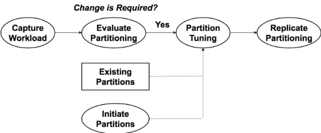
that preserves contiguity at each step to avoid expensive contiguity checks and contiguity repair operations [Liu et al., 2016]. This incremental approach to tuning existing partitions avoids creating partitions from scratch, which is clearly inefficient [Aly et al., 2015] and works by moving a limited number of spatial units among partitions to re-balance them. Hence, our approach is able to autonomously scale-in when some partitions are underloaded and scale-out when some partitions are overloaded. The overall process of our adaptive partitioning algorithm is explained in Figure 1.2.

Figure 1.2: Adaptive workload-aware partitioning process.

To avoid disrupting the data ingestion/retrieval process while migration is happening, we provide a rolling migration process among partitions by simultaneously holding two versions of the partitioning (existing and future partitioning schemes), each differentiated by the timestamps of the data they are holding. By using this technique, we do not interrupt the operations of the framework while partition modification is in progress.

We evaluate the effectiveness of our partitioning approach by using an integrated dataset that contains one year of Twitter geo-tagged tweets. In addition, we inject randomly gen-erated hotspots into the dataset to simulate inevitable changes in the underlying workload. Our experiments demonstrate the advantage of our adaptive partitioning approach over pre-viously used static partitioning methods such as k-d tree, in terms of load balance metrics and cost of changing partitions. Finally, we evaluate scalability by measuring latency and throughput of our approach using a varying number of partitions and nodes.

(18)

1.1.2 Thesis Layout

In the first part of the thesis, we explain the motivating case studies for the algorithmic and architectural innovations that are elaborated in Chapter 2. The case studies include multiple data-driven geospatial applications encompassing the four main components of cyberGIS data-driven workflows, i.e. data management, data integration, data-driven computing and interactive analytics.

Chapter 3 explains our approach to workload-aware load-balancing of data-intensive geospa-tial applications. We evaluate our load-balancing approach using two case studies: move-ment aggregation and point-in-polygon. We report the load statistics for both operations to demonstrate the load balancing effect of our approach. In addition, for both operations we evaluate the “interactive scalability” of the associated workflow by performing stress test with multiple types of queries.

In the next two chapters, we shift our focus into adaptive partitioning of data for applica-tions that handle streaming data. In Chapter 4 describes a geohash-based model for indexing geospatial data. This model is particularly beneficial for solving our problem since it can be efficiently stored and retrieved using key-value data stores and can be updated concurrently for high-velocity. Since geohash is primarily used to index points, we have developed two efficient algorithms to index polygons and lines using geohash.

Chapter 5 describes a novel algorithm for adaptive partitioning of geospatial data. We model the problem of finding the optimal partitions as a spatial optimization problem with the multi-criteria objective function including load imbalance deviation and spatial com-pactness (Section 5.3). This algorithm can gradually modify the partitions by performing a spatially tuned mutation operation (Section 5.6). Section 5.7 highlights the advantages of our adaptive partitioning approach compared to a static partitioning method and other adaptive partitioning methods (e.g. Kd-Tree).

(19)

described in Chapter 5 to efficiently manage high-velocity real-time geospatial data. Partic-ularly, GeoBalance is based on a microservice-based architecture (Section 6.2) that integrates a number of distributed and loosely connected services. In addition, we articulate how spa-tiotemporal workload is modeled in GeoBalance (Section 6.3) according to the statistics reported from multiple nodes.

Finally, in Chapter 7 we conclude this dissertation by summarizing the overarching re-search contributions. In addition, we discuss the future rere-search directions related to optimal partitioning of geospatial data for cyberGIS analytics.

(20)

CHAPTER 2 MOTIVATING CASE STUDIES

This chapter reviews multiple related cyberGIS applications, which serve as the motivation for the algorithmic and architectural innovations that will be discussed in the following chapters. While each application serves specific analytical purposes, its associated algorithms are designed in a generalized fashion and may be applied to similar problems. For instance, UrbanFlow [Soltani et al., 2016] reveals intra-city human mobility patterns by combining real-time social media data with authoritative landuse maps through a generic spatial data synthesis approach that addresses one of the major problems in distributed spatial data processing [Eldawy, 2014]. All of the following applications have been implemented within a cutting-edge CyberGIS Gateway software environment [Liu et al., 2015, Wang et al., 2016].

2.1 MovePattern

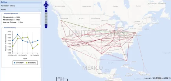
MovePattern [Soltani et al., 2015a] is designed to achieve interactive and scalable visual-ization of massive movement datasets, where movement is defined as a trajectory between source S and destination D in time T. For instance, consider the movement of Twitter users throughout the United States in the August of 2014 which was close to 76 million movements. If we would visualize all the movements on a map, the end result could be too cluttered (and computationally expensive to generate) to present any useful information [Liu et al., 2013]. MovePattern aims to resolve this challenge by efficiently generating a multi-resolution view of the movements, providing various levels of details as users interactively explore patterns of data visualization (Figure 2.1).

(21)

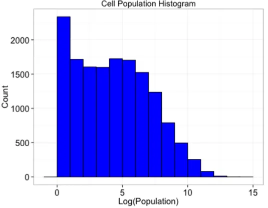
The aggregation and summarization methods of geographical movements are implemented using the well-known distributed MapReduce model [Dean and Ghemawat, 2008] to provide seamless scaling for massive movement datasets. However, real-world geospatial datasets usually have heterogeneous spatial distributions [Soltani et al., 2015a]. For instance, Figure 2.2 reveals that the frequency of geo-tagged Twitter data in different locations follows a long tail distribution. Therefore, our MapReduce algorithms take the skewed distribution of data into consideration and devise an efficient scheme to balance the data and computation load among parallel computing units. In Section 3.2, we will detail our approach to address the spatial skew of movement data.

Figure 2.1: MovePattern web application

In addition, MovePattern emphasizes the importance of considering the workload of han-dling user-driven visualization requests (Section 3.2.3), which was generally overlooked in previous work [Zinsmaier et al., 2012, Daae Lampe and Hauser, 2011]. For instance, to eval-uate the interactivity of the framework we used two different access patterns: 1) random access pattern and 2) focused access pattern. While the first pattern focuses on randomly generated user requests, the second one is modeling real-life scenarios where many users ac-cess a focused section of data, e.g., due to hotspots caused by common attention to certain locations.

(22)

opposed to pixel-based approaches that were used in previous work [Zinsmaier et al., 2012]. In a pixel-based approach movement information is not straightforward to be linked back to the original data, making it impossible for users to get specific information about individual nodes/edges after a visualization product is presented. Therefore we use a vector-based approach to increase the analytical capabilities of the framework.

Figure 2.2: Number of Tweets from Oct-Dec 2014 in a Uniform Grid with32km×

32km Cells covering the Continental United States.

2.2 GeoHashViz

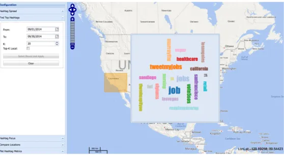
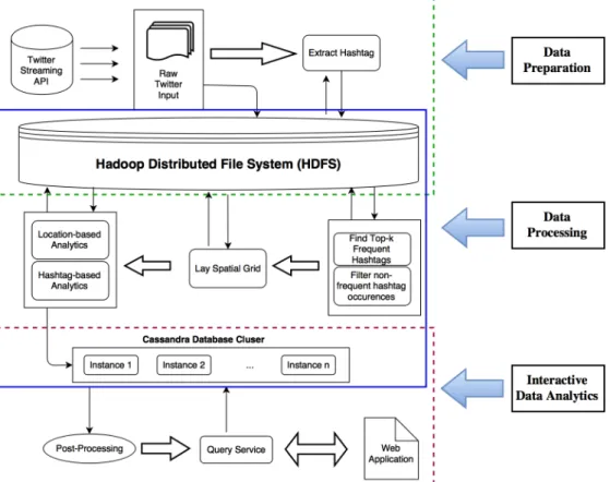
GeoHashViz [Soltani et al., 2015b] provides interactive analytics for understanding spa-tiotemporal diffusion of Twitter hashtags (Figure 2.3). Recent research studies have con-firmed that Twitter hashtags can be used effectively to track diffusion of ideas including social memes, political trends and social movements [Kamath et al., 2013]. Hashtags are

(23)

proven to be more explicit and less noisy than the actual text of tweets, thus an effective medium to study collective diffusion of ideas in the virtual world [Romero et al., 2011,Kamath et al., 2013, Chang, ]. GeoHashViz provides two types of analytics: 1) hashtag-based (spa-tial spread, focus points and spread metrics) and 2) location-based (Top-k popular hashtags, compare regions). Such analytics requires a series of pre-processing steps, implemented us-ing Apache Hadoop and a highly interactive module that queries the result of pre-processus-ing steps and generate analytical outcome.

A key challenge of this research is to model diffusion of ideas using spatially-aware metrics. For instance, to find the top-k popular hashtags in a selected region, we should query the selected region, aggregate the hashtags by count and select the most popular ones. However, this often might lead to a limited set of hashtags which are globally popular (e.g. #jobs) and does not provide any valuable insight into that region. Therefore, we employed a Tf-idf like metric [Sheng et al., 2010] to find the hashtags that are specifically popular in that region. The first part of the metric, called CF −IRFh,C(t) is to define hashtag frequency. Suppose

thatOh_l(t) is the frequency of hashtag l in locationh at timet. Then, the hashtag frequency for geographical boundC is defined as:

CFh,C(t) = P l∈COhl(t) P l∈COl(t) (2.1)

Now we focus on the importance of hashtag h in C which relates to the distribution of locations which have used h over the entire region of study. We lay a gx×gy uniform grid

on top of data points. Similar to the definition of Oh

l we define Ogh as the occurrences of

hashtag h in the gird cell g. Now we can define the hashtag importance as:

IRFh(t) = log

|gx×gy|

|{Oh

g(t)|Ogh(t)6= 0}

(24)

The final metric is then formulated as:

CF −IRFh,C(t) =CFh,C(t)×IRFh(t) (2.3)

By calculating this metric for all the hashtags that have appeared in boundCat time period

Figure 2.3: Visualizing top-k frequently used hashtags in a selected region using GeoHashViz web application.

of t, we can find the top−K locally significant hashtags.

GeoHashViz requires access to massive records on a hashtag or a location. Therefore, to ensure the interactivity of the framework, we pre-compute some analytical features of hashtags and locations and combine them on-demand to answer user queries (Figure 2.4). The result of the pre-computation step is stored using a denormalized data model. The data model employs the denormalization optimization principles to reshape the data and store multiple copies of data grouped and indexed differently (according to the users workload) to provide faster read performance and avoid costly joins.

(25)

Figure 2.4: Architectural pipeline of GeoHashViz that includes pre-computing steps and on-demand services.

(26)

2.3 UrbanFlow

Recent work suggested that geo-tagged tweets are complementary sources of information to characterize urban landuse types [Frias-Martinez and Frias-Martinez, 2014]. Patterns ex-tracted from geo-tagged tweets such as relative changes in number of tweets, number of users and user movements were found to correlate with the urban activity patterns [Wakamiya et al., 2011]. These interesting results motivate the development of open platforms for ana-lyzing massive geo-located datasets. The demand for these platforms is high because of the need to monitor and understand urban dynamics.

However, the lack of accurate user activity context, makes it challenging to use geo-tagged social media data in urban dyanmics studies. UrbanFlow [Soltani et al., 2016] is designed to solve this problem by integrating social media data with traditional authoritative data sources such as landuse maps. For example, using UrbanFlow, researchers are able to find users’ most frequently visited locations through spatial clustering and determine their context by integrating those locations with their corresponding landuse types (e.g. home, work, education, etc.). UrbanFlow provides visual insights to help understand urban spatial networks based on identifying common frequent visitors between different urban neighborhoods (Figure 2.5).

UrbanFlow includes a novel distributed approach to synthesizing spatial data in a dis-tributed fashion using the MapReduce programming model. The integration problem in Ur-banFlow can be solved through a classic point-in-polygon algorithm, while each geo-located tweet is represented as a point and each land parcel is represented as a polygonal area. This algorithm resolves the limitation of previous approaches [Zhang et al., 2015, esr, 2013] that only treat small or modest sizes of landuse datasets. In addition our approach sustains the inaccuracy in both polygon mapping and GPS locations by integrating points with their nearest polygon if an exact match does not exist. In Section 3.3, we describe the distributed approximated point-in-polygon algorithm used in UrbanFlow.

(27)

(a) Time series plot for number of tweets per hour of the day and day of the week for each landuse type

(b) Stack plot of dominant land use for top vis-ited locations grouped by rank, confirming the high preferential bias to tweet from residential specially for top locations (rank1)

(c) box plot of clustering purity with most of the clusters corresponding to a single land use parcel (purity = 1.0)

Figure 2.5: Visual analytics in UrbanFlow’s web application [Soliman et al., 2017]

(28)

UrbanFlow has been used by other researchers as an example of complex distributed geospatial applications to examine cloud operation management platforms and study scal-ability patterns. In one example [Keahey et al., 2017], researchers used UrbanFlow to test their operation management platform for multi-cloud environments. As another example, UrbanFlow was profiled in detail [Fu et al., 2018] to evaluate multiple dynamic data redis-tribution mechanisms in Apache Hadoop.

2.4 CyberGIS-Fusion

CyberGIS-Fusion is developed to demonstrate CyberGIS capabilities for a large number of users to perform computing and data-intensive, collaborative geospatial problem solving enabled by advanced cyberinfrastructure. The main contributions of CyberGIS-Fusion are:

• Provide a fast and scalable framework to insert/retrieve spatiotemporal data.

• Synthesize heterogeneous geospatial datasets in a single integrated environment.

• Facilitate seamless integration of multiple microservices to take advantage of cloud infrastructure.

To evaluate CyberGIS-Fusion, we chose the Beijing Taxi dataset1 which includes more than 15 million taxi trips in Beijing from Feb 3rd to Feb 9th 2008 (Figure 2.6).

CyberGIS-Fusion is an example of real-time geospatial applications, where the ingestion-rate is high and the data should be immediately available to be queried. This is funda-mentally different than batch-processing systems such as Apache Hadoop [Shvachko et al., 2010a]. Batch processing systems, while capable of dealing with massive datasets, are not tailored to handle real-time data where bulk loading of the data is not feasible.

One major challenge in designing a scalable data management framework for handling highly dynamic real-time data is related to how the data is distributed among different

(29)

Figure 2.6: CyberGIS-Fusion web application for accessing Beijing taxi data.

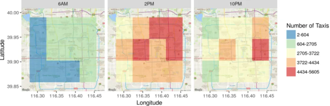
nodes. Throughout the development of CyberGIS-Fusion we observed that geospatial data distribution may vary significantly over time (Figure 2.7), hence an effective partitioning scheme can dramatically improve the resource utilization and throughput of CyberGIS-Fusion. Particularly, we focus on adaptive workload-aware partitioning that a) uses both query and data distribution in determining the optimal partitions and b) adapts to changes in the data and query distribution over time. In Chapter 5, we discuss the algorithms for adaptive workload-aware partitioning of real-time geospatial data.

(30)

Figure 2.7: Changes in spatial distribution of taxi data over different hours of the day in the City of Beijing.

(31)

CHAPTER 3 STATIC WORKLOAD-AWARE LOAD BALANCING

FOR DATA-INTENSIVE GEOSPATIAL

APPLICATIONS

3.1 Overview

Geospatial scientists have taken advantage of advanced cyberinfrastructure to solve computation-and data-intensive problems [Wang et al., 2005]. Traditional research in this area focused on using high performance computing to design scalable algorithms and frameworks [Tang et al., 2011, Liu and Wang, 2015]. However, the focus has shifted dramatically in the past decade to cloud-based approaches [esr, 2013, Soltani et al., 2016]. Particularly in the case of data-intensive applications, cloud computing provides scalable functionalities to distribute geospatial data and parallelize spatial operations through exploiting data parallelism.

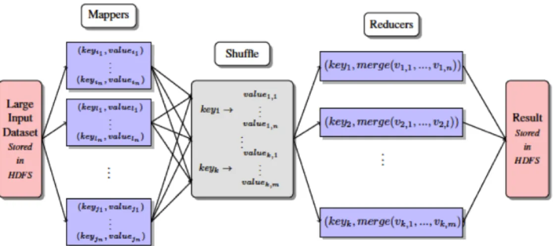
MapReduce has been adopted as a major programming paradigm of cloud computing [Dean and Ghemawat, 2008]. The paradigm contains two main steps: map and reduce. In the map phase input data is converted into series of intermediate (key, value) pairs. Then after shuffling and sorting the intermediate pairs, the reduce phase will collect all the (key, value) pairs that have the same intermediate key (Figure 3.1). This programming framework can support automatic parallelization as the map operations are considered independent and can be done in parallel. In addition, MapReduce can scale horizontally by seamlessly adding new computing nodes for data hosting and processing.

Hadoop [Shvachko et al., 2010b] is an open-source implementation of MapReduce, which is built on top of a distributed file system called Hadoop Distributed File System or HDFS. Hadoop facilitates data-intensive computing on large commodity clusters by providing ca-pabilities such as data distribution, parallel computing and fault tolerance. From early

(32)

Figure 3.1: MapReduce programming model.

days of Hadoop, geospatial communities have embraced the framework and used it to solve data-intensive problems [Cary et al., 2009b, Liu et al., 2010]. However, previous work has also proved that adapting spatial algorithms to the MapReduce programming model is a challenging task [Eldawy and Mokbel, 2015]. First, Hadoop takes advantage of functional programming model which requires fundamentally different thinking on how to design opti-mized algorithms. In addition, Hadoop does not natively exploit spatial data characteristics. Therefore, customized techniques need to be designed to handle distributed processing of spatial data in the Hadoop ecosystem.

Previous research has extensively studied the issue of data partitioning and indexing on Hadoop [Eldawy and Mokbel, 2015]. The main challenge regarding distributing spatial data in Hadoop is the fact that data in HDFS works in an append-only fashion and data in HDFS is immutable. To address this limitation, researchers have suggested to use a sample of the data to build the index prior to storing the data in HDFS [Eldawy, 2014]. The index is built in two different granularities: the global index that is accessible to all parallel workers and the local index that is built locally for faster spatial operations. Using the two-level indexing scheme, whenever a spatial operation has to be performed, the system can find the associated data blocks using the global index and find corresponding answers by looking into the local index of the data blocks. While the overall design stays the same, different

(33)

researchers have used different indexing algorithms such as uniform grid [Aji et al., 2013a], Z-curve [Cary et al., 2009a], R-tree [Eldawy, 2014] or quadtree [Eldawy et al., 2015b].

Compared to extensive work on partitioning and indexing methods for static geospatial applications, limited work has been done to consider expected workload into such approaches. As previous researchers indicated the tight coupling between spatial domain decomposition and task scheduling is problematic due to the inability of this approach to scale for new data sources, operations and architectures [Wang and Armstrong, 2009]. Therefore, solely focusing on data and operations is “logically inappropriate” for designing efficient domain decomposition and task scheduling strategies [Wang and Armstrong, 2005]. We attempt to address this issue by introducing workload and focusing on problems that are sensitive to workload and more concerned with the variability of the computational tasks that are applied to the data, rather than the distribution of the data. Specifically, we study the methods and algorithms for spatial computational domain representation, using two well-known examples: 1) multi-resolution data aggregation and 2) approximate point-in-polygon problems. This study will complement the previous effort on using Hadoop for geospatial problems by shedding light on a new dimension of distributed processing of geospatial data. One of the most significant issues in MapReduce applications is to deal with skew [Kwon et al., 2012]. While in Hadoop, input data is evenly distributed among mappers, based on the configuration variable dfs.block.size, the applications can still suffer considerably from skew among reducers. The reason for existence of such skew is the inability of Hadoop to dynamically balance the load among reducers. Particularly real-world spatial data are usually highly skewed and therefore a custom partitioner is required to balance Hadoop-based computation. This skew is beyond the distribution of the original data and more related to how the computation model is defined. Similar to the definition of computational intensity, the problem of skew relates to spatial domain decomposition, spatial operations as well as the distribution of data. Therefore, to avoid load imbalance we have to consider the computational intensity of the problem in designing distributed algorithms [Soltani et al.,

(34)

2015a].

Our approach has two main steps. First, we use either a theoretical analysis of the problem or a sample of workload to generate a computation plan. This will define how the computation is going to be divided among reducers and is similar to the global index which have been used in previous research. This step may be accompanied by spatially aware partitioning of input data [Soltani et al., 2016]. Second, we use the computation plan to run its corresponding MapReduce job. In the mapper stage, we use the global index to determine which reducers the data should be assigned to. Furthermore, the reducers will receive their portion of data, performs pre-processing steps such as spatial indexing and and compute the final result.

The generation of a computation plan can be understood as a spatial computational domain decomposition problem that is defined based on the nature of the problem and computational intensity analysis of it [Wang and Armstrong, 2009]. This analysis may vary from problem to problem. Therefore we cannot solely rely on a fixed data distribution scheme, as done by some previous work [Eldawy, 2014, Aji et al., 2013a], and thus have to consider a mechanism that can provide the decomposition for each problem (workload-awareness). The computational intensity relies on the spatial distribution of data, complexity of spatial operations, as well as surrounding geographical regions in some cases. Therefore, the approach should be able to handle possibly overlapping regions for the decomposition. In the rest of this chapter, we elaborate our approach by using two case studies.

We evaluate our approach from three different perspectives. First, we study the advantage that our approach provides in terms of reducing the computational and data skew among reducers. Particularly, we study how reducers’ data and computational loads are affected by taking advantage of our spatial computational domain representation. Our second experi-ment is focused on determining the optimal granularity for our spatial domain decomposition, which is a critical issue for large-scale geospatial applications [Wang and Armstrong, 2009]. On one hand, the granularity should be coarse enough that justifies the computational

(35)

ben-efits of decomposition, compared to the overhead of parallelization. On the other hand, the granularity should be sufficiently fine to allow for sub-domain to be processed in parallel. Therefore, we evaluate our approach in both examples against multiple granularities to de-termine the most efficient setting. Finally, since both examples are designed to be interactive applications, we conduct experiments by simulating expected workload on the applications. The goal of these experiments is to ensure that interactivity of the applications stay intact under both temporally and spatially intense query workloads.

3.1.1 Geo-tagged Twitter Data

In both applications we heavily rely on geo-tagged Twitter data to demonstrate the value of our approach. We collect geo-tagged tweets using a custom crawler specifically designed for collecting tweets containing geographic coordinates or place information using Twitter’s open access streaming API. The crawler records user id, location, time, text and some associated flag variables (e.g. whether the tweet is a retweet). We exclude data outside of the North American continent and collections over 2.5M tweets on a daily basis.

3.2 Movement Aggregation and Summarization

3.2.1 Background

Large amounts of data pose unique requirements for generating visualization in a scalable fashion. Liu, et al. [Liu et al., 2013] formulate this problem by distinguishing the “interactive scalability” from “perceptual scalability”. Perceptual scalability means avoiding plotting every possible point so that users are not overwhelmed. Interactive scalability means that the visualization provides fast responses to multiple users queries and eliminates long latencies in user interaction. Data reduction techniques and detail-on-demand capability [Shneiderman, 1996] can provide an answer to the perceptual scalability problem [Zinsmaier et al., 2012].

(36)

However, we still may experience significant latency in the user queries that negatively affect the user experience. Therefore, it is a common practice in large-scale visualization systems to reduce query time by offloading some computation to the server side and adding a pre-processing step [Keim, 2005, Liu et al., 2013].

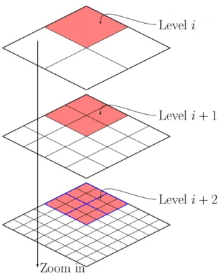
Previous studies explore three groups of reduction methods for spatial movement data: clustering, density-based and binned aggregation. Clustering approaches [Guo, 2009, Jia et al., 2011] re-model the problem as a graph community detection problem which enables them to define multiple level of abstractions for the movements. However, these approaches tend to perform poorly on large datasets, since they require calculating modularity be-tween large numbers of nodes. Density-based approaches use kernel density estimation with adaptive bandwidth to provide multi-scale view of the movement graph [Zinsmaier et al., 2012, Daae Lampe and Hauser, 2011]. In contrast to clustering methods, density-based ap-proaches are usually very fast due to the fact that they can be efficiently implemented using GPU. However, these methods employ a pixel-based approach where the visualization cannot be linked back to the original data. Therefore the user cannot get specific information about the edges after the visualization is produced. Binned aggregation is another approach which defines the aggregates of the data based on pre-defined spatial bounds [Liu et al., 2013]. One main advantage of this approach is that it can be easily parallelized over multiple computing nodes [Eldawy et al., 2015b]. In addition, binned aggregation can form multiple views of data using a hierarchical definition of bins. For demonstration of this work we adapted a form of binned aggregation, known as hierarchical spatiotemporal data cube [Cao et al., 2015] (3.2), which has been used to model multi-resolution movements [Padmanabhan et al., 2014]. However, the framework is not limited to this data model and can be easily applied to other binned aggregation data schemes as well.

(37)

Figure 3.2: MovePattern employs hierarchical data cube model.

3.2.2 MapReduce Algorithms for Movements Aggregation and

Summarization

In the MovePattern framework [Soltani et al., 2015a], there is an important need for process-ing geographical movements and produce a multi-resolution view of collective movements. This includes three main steps:

• Aggregate the movements based on a hierarchical data model.

• Summarize the aggregated graph by eliminating nodes that are not deemed as ”signif-icant” compared to their local neighborhood.

• Filter edges associated with nodes that are filtered out in the previous step (using Bloom Filter [Bloom, 1970]).

To build the spatial decomposition scheme, we used the recursive bisection approach that partitions a space into a set of rectangles [Berger and Bokhari, 1987]. In this method at each

(38)

step, we divide the region into two sets to minimize the imbalance. One main variation of our approach from the original recursive bisection method is that instead of alternating the cut axis at each level, we choose the axis that achieves better balance among two sets.

The result spatial decomposition scheme is saved on HDFS and can be loaded at the beginning of each MapReduce job, and indexed using R-tree, to determine how the compu-tation is assigned to corresponding reducers. Algorithms 1 and 2 are examples of mapper and reducer stage using this approach.

Algorithm 1: Mapper for spatial aggregation

function mapper(movement)

s ←movement.source ;

t ←movement.target; for l= 1...Ldo

id1←getCellId(s, l) ;

id2←getCellId(t, l) ;

merge(graphs[l], id1, N ode(s,1)) ;

merge(graphs[l], id2, N ode(t,1)) ; if d(s, t)< threshold(l)then

merge(graphs[l], id1, Edge(id1, id2,1)) ;

function cleanup()

for l= 1...Ldo

foreach key in graphs[l] do

p←rtree.search(key) ;

emit(p,[l, graphs[l].get(key)]) ;

Algorithm 2: Reducer for spatial aggregation

function reducer(key, Node[] values)

foreach value in values do

merge(graphs[value.level], value.id, value) ; for l= 1...Ldo

foreach key in graphs[l] do

x←graphs[l].get(key) ;

write(“N odes00, x.level, x.coor, x.count) ;

(39)

While multi-resolution spatial aggregation provides a generalized view of data, it can be still too large to convey any clear patterns to users in a visualization interface. For instance, if we divide North America into 512km×512km cells, we will end up with 468 grid cells which can have up to 109278 edges among them. Therefore, even for very coarse-level view of data, we get a very cluttered graph; hence the result from node aggregation step needs to be summarized for a less cluttered visualization.

Our summarization technique filters less “significant” nodes (grid cells) by assigning them a score, reflecting how large their degree is comparing to neighboring cells. Then by compar-ing the score to a pre-defined threshold we can decide whether to keep or drop a node from the graph. As previous research has pointed out [Padmanabhan et al., 2014] geographical distribution of real-life location-based data is highly skewed, with a small number of places contributing most of the activities. Therefore, the definition of “significant” nodes should be localized to their surrounding sub-regions as opposed to using the same significance measure for the whole region of study.

The local neighborhood of point p is defined as {q ∈ P : d(p, q) < r}. Here P is the set of all points in the graph (in the same spatial resolution as p), d(p, q) is the great-circle distance between p and q and r is the neighborhood radius (Figure 3.3). By reducingr we will have a more strict definition of a neighborhood which will lead to having more points in the final graph. The value of r can be adjusted for each spatial resolution.

Using the neighborhood formulation, calculating local rank can be simply defined as the percentile rank of point p inneighborhood(p):

localranking(p, neighborhood(p)) = Σq∈neighborhood(p)cf(p, q)

|neighborhood(p)| (3.1) Where: cf(p, q) =      1 ifdegree(p)≥degree(q) 0 otherwise (3.2)

(40)

To model this problem using MapReduce, we have to be cautious to avoid unnecessary com-munication among different nodes. In the naive approach each node send their information to every other node, and help them find about their neighborhoods. However, this will lead to very expensive communication overhead. Instead we take advantage of the partitioning scheme that was built in the initial stage of the data processing module to prune many choices and end up with only a small set of cells as neighbor candidates. The uniform structure of the grid enables us to easily extract the set of cells, which are in a certain distance from the current cell. The outline of this MapReduce based approach is explained in Algorithms 3 and 4. The input of this job is the “Node” output of the aggregation step.

Figure 3.3: MovePattern requires a summarization step to eliminate insignificant geographical nodes.

3.2.3 Experiments

To evaluate our approach, we designed an experiment on processing movements from Twitter users starting August 1st, 2014 through October 31st, 2014 (Table 3.1). The tweets were collected and geo-referenced based on the Twitter Streaming API [Padmanabhan et al., 2014] and movements generated by forming a spatiotemporal trajectory for each user. To

(41)

Algorithm 3: Node Summarization Mapper

function getNeighborPartitions(node, level)

of f set ←cell len[level]×r[level] ; result-set ←rtree.f indN eighbors(

node.coor, of f set) ; return result-set ;

function mapper(node)

foreach p in getN eighborP artitions(node, node.level)do

emit(p, node) ;

Algorithm 4: Node Summarization Reducer

function reducer(key, Node[] values)

for l= 1...Ldo

rtrees[l]← new rtree() ; foreach node in values do

if !rtrees[node.level].contains(node) then

rtrees[node.level].add(node) ; for l= 1...Ldo

foreach node in rtrees[l] do

of f set←cell len[node.level]×r[node.level] ; result-set ←rtrees[node.level].f indN eighbors(

node.coor, of f set) ;

rank ← percentile rank ofnode.count inresult-set ; if rank ¿ threshold then

write(”SummaryN ode”,

(42)

divide the data into multiple spatial resolutions, a hierarchical uniform grid is formed with 10 levels, representing different levels of details for the North America continent. At the finest level, a uniform grid with cell size of 30 arc seconds (approximately 1 km × 1 km) is formed and the cells are iteratively merged to form the uniform grids on the higher level. The merging operation is done in an exponentially increasing fashion forming cell sizes of 2, 4, . . . , 512 km. In addition, each cell is presented using the centroid of all the points (location of tweets) within the cell.

The experiments were conducted on the cyberGIS supercomputer called ROGER1 su-percomputer at the University of Illinois at Urbana-Champaign. For the Hadoop cluster, we used 8 nodes each including 2 Intel Xeon E5-2660 2.6 GHz CPU (20 cores total), 256 GB of memory and 800GB of SSD hard drive. In this section, we present only two of the experiments (see the original paper [Soltani et al., 2015a] for more experiments). First, we evaluate our spatial decomposition method to test the load on each reducer. Table 3.2 shows the statistics on reducers load when aggregating data for the 3-month dataset. This result confirms that using the spatial decomposition method, described above, we can divide our study space into multiple regions with similar computational load, which as we explained is a critical issue in designing MapReduce-based algorithms. The next experiments focus on the performance of spatial aggregation and summarization methods against the three test datasets. Table 3.3 shows how aggregation and summarization methods affect the number of locations and movements among them. These two experiments demonstrate the ability of our approach to scale and dramatically reduce the movement graph size by intelligently aggregate movements in multiple resolutions.

Duration Tweets Users Movements Size(GB)

1-month 107M 2.2M 76M 2.77

2-month 205M 2.9M 136M 5.43

3-month 368M 3.5M 179M 9.88

Table 3.1: Input data statistics

(43)

# of Reducers Avg Std Min Max 8 5,853,967 120,348 5,709,732 6,037,848 16 2,926,984 73,670 2,821,192 3,096,001 32 1,463,492 58,673 1,344,301 1,609,537

64 731,746 45,466 654,939 846,538

Table 3.2: The reducers’ load statistics in terms of associated keys to each reducer.

Dataset Nodes Edges

1 month 2.67M →939K 33.98M →4.66M

2 months 3.18M →1.08M 49.27M →6.88M

3 months 3.48M →1.16M 59.55M →8.44M

Table 3.3: Combined Effect of aggregation and summarization on graph size

Interactive Scalability

To evaluate interactive scalability, we simulate two categories of queries that represent two most common query patterns of users:

1. Population Query Pattern: Queries are distributed in a weighted fashion around the region of study (here North America) with more queries on sub-regions with higher number of tweets.

2. Hotspot Query Pattern: Queries are focused on a specific relatively small region resembling occasional situations which an outburst will lead to large number of focused access. For instance, a political visit or a natural disaster can attract user attentions to a certain area.

The underlying assumption in both access patterns is that the framework is likely to get more queries from regions where there are more tweets. Therefore, we generated the query bounding box according to a sample of tweets, where more crowded regions are more likely to be presented in the sample. In addition, the spatial resolution is randomly chosen in a uniform fashion from{1,2, ...,10}.

(44)

For our experiments, we generated 3 sets of 2000 queries for overall and focused query pat-tern. Then Apache JMeter2_{, a load testing tool, is used to send this queries to MovePattern} with different rates of queries per second and the response time is measured. We launched 2000 queries in the duration of 50, 75 and 100 seconds, on the 3-month dataset. After per-forming aggregation and summarization, this dataset contains over 1.16M nodes and 8.44M edges. Table 3.4 shows statistics (average, median and 90% percentile) on the response time of queries for both normal and focused patterns. The result shows that MovePattern can sustain relatively large number of simultaneous queries, each based on different resolutions and regions.

Population Pattern

Duration(s) Average Median 90% Percentile

50 42 29 96

75 34 23 79

100 31 21 72

Hotspot Pattern

Duration(s) Average Median 90% Percentile

50 36 24 82

75 31 21 69

100 28 19 63

Table 3.4: Stress test for 2000 queries on 3-month dataset (in ms)

3.3 Distributed Approximate Point-in-polygon

3.3.1 UrbanFlow Architecture

UrbanFlow collects input data using the Twitter Streaming API [Padmanabhan et al., 2014]. In the first step, two filters are applied to tweets: 1) spatiotemporal filter: to filter tweets

(45)

based on spatial extent and timespan of the study and 2) user filter: to filter tweets from users with very low engagement, indicating a very sparse present over time. The second filter is particularly critical, since we want to capture actual mobility patterns of people and eliminate inactive users with noisy behaviors.

In the next step, the processed tweets dataset is integrated with authoritative dataset using our novel distributed point-in-polygon algorithm (refer to Section 3.3.2). Then we identify frequently visited locations of each user (Section 3.3.1). Finally the clusters are joined with the user-defined partitioning scheme to enable region-based analytics. All the above steps are implemented using Apache Hadoop. Figure 3.4 demonstrates the architecture of UrbanFlow.

Figure 3.4: UbranFlow Architecture

Identifying Frequently Visited Locations

Previous studies have indicated that human mobility patterns can be explained by preferen-tial return to few frequently visited locations (FLV) such as home, work, school, etc [Soliman et al., 2015]. There are multiple methods to identify the FLVs, ranging from simple solutions such as imposing a fixed grid on the users’ locations [Cao et al., 2015] to more advanced methods such as spatial clustering techniques [Bora et al., 2014]. We identify FLVs by using DBSCAN clustering algorithm [Ester et al., 1996] on each user’s recorded locations.

(46)

DB-SCAN method does not assume a predefined number of clusters or any particular spatial shape. This is particularly beneficial for our application, due to heterogeneous nature of human mobility. The result of this step is a series of clusters per user, marked by their spa-tiotemporal characteristics as well as their rank in the user’s everyday activities. The rank of a cluster demonstrates the tendency of the user to return to that FLV and determined based on the number of tweets in the cluster. For instance, for most of the users the first rank cluster is considered as home, while work/school may appear in the lower ranks [Soliman et al., 2015].

We also introduce the purity metric of clusters, to evaluate the choice of clustering pa-rameters. The purity of a cluster is defined as the frequency of the most common landuse parcel to total number of points in that cluster. For instance, the purity of 1.0 indicates that the cluster is completely located in/near one land use parcel. For a reasonable choice of clustering parameters, we expect the most clusters to have high purity number.

3.3.2 Point-in-polygon Approach

Spatial Decomposition Method

UrbanFlow [Soltani et al., 2016] implements a scalable point-polygon algorithm that in-tegrates geo-tagged tweets with fine-resolution authoritative landuse data. There are two main challenges in designing such algorithms in a distributed fashion. First, in addition to the large point dataset (tweets), our polygon dataset is also large and may contain hundreds of thousands of polygons. Previous work on this problem [Zhang et al., 2015, esr, 2013] suf-fered from the inability to scale when the number of polygons is large. This limitation is due to the fact that these methods attempt to send all the polygons to every worker, which is clearly inefficient for large number of polygons. In other word, these approaches only exploit the parallelism to the points dataset. Second, due to the existence of noise and inaccuracy in both measurements and movement patterns of humans, the approach should be able to

(47)

approximate point-in-polygon process to assign points to desirably close polygons, in case an exact match does not exist (Figure 3.5).

Figure 3.5: Example of inaccuracy in human mobility patterns: the geo-tagged location of tweet may not perfectly match with the building that the user is associated to. Our approach will assign the geo-tagged tweets to its closest land parcel if an exact match does not exist.

To address the above issues, we developed the following approach. First, we pre-process the polygons and break them into smaller spatially contiguous chunks. This step is in-terleaved with the spatial decomposition method. Therefore, for each decomposition, the corresponding polygons that overlap with the region is determined as saved to a separate file in HDFS.

Second, we expand the original point-in-polygon operation to find the closest point-in-polygon. The goal here is to find the polygon that is closest to a given point, considering a distance threshold (minDist). Let’s consider point p which lies into partition i with bounding boxBBi . Ifpmatches a polygon that is presented in partitioni, our work is done

(no approximation required). However, in casepdoes not match any polygon in partition i, we should look for the polygon that has the minimum distance top. The main issue is that in partitions’ boundaries, this polygon may not intersect with BBi . We resolve this issue

(48)

minDist of bounding box BBi . While we expand the polygons in partitionp beyond BBi

, we will not change the representative bound of partition i. This guarantees that a point will match with one and only one partition. Otherwise an expensive post-processing step is required to handle points that are associated with multiple partitions. Figure 3.6 illustrates this process.

The Algorithm 5 explains the process of splitting the original polygons into smaller sets. The division criteria (getP artitionW ithHighestCI) is defined by the user according to the desired model for computational intensity of the problem. Some candidates are number of polygons, number of points based on a sample of data or the area of the region. We also takes advantage of Median of Medians algorithm [Blum et al., 1973], which can calculate the median of an array in linear time. In addition, Algorithm 6 explain how the splitting algo-rithm is employed to generate computational spatial domain decomposition among reducers.

MapReduce Algorithms

Once the spatial decomposition is devised, a MapReduce job is designed that reads the space decomposition index in the mapper stage and determines which reducer should receive the point. The reducers (Algorithm 8) take care of the main point-in-polygon process. Each reducer reads and indexes its associated partition only once and then use that to find the closest polygon associated with each point. The spatial indexing (for bounds and partitions) are done using R-tree.

3.3.3 Experiments

We conducted an experiment using geo-tagged tweets from January 2013 to January 2016 (2.42 billions of tweets for US boundaries) and filtered them to only keep tweets that match Chicago’s bounding box (nearly 47 million tweets). To identify the landuse type of each

(49)

Figure 3.6: Example of splitting space into 4 partitions, illustrating how each partition includes more polygons than its representative bounding box (colored rectangles) to enable closest point-in-polygon operation. The non-filled rectan-gles show the bounding box of all the polygons in each partition.

(50)

Algorithm 5: Split original polygons into partitions

function divideBounds(partition, divideDirection)

coordinates ←partition.polygons.centroid[divideDirection] ;

median ←M edianOf M edians(coordinates) ;

newBounds←newArray() ;

if divideDirection is x−axis then

newBounds[0]←

[partition.minX, partition.minY, median, partition.maxY] ;

newBounds[1]←

[median, partition.minY, partition.maxX, partition.maxY] ; else

newBounds[0]←

[partition.minX, partition.minY, partition.maxX, median] ;

newBounds[1]←

[median, median, partition.maxX, partition.maxY] ; return newBounds ;

function split(partition, threshold)

divideDirection←

alternate(parition.divideDirection) ;

newBounds←

divideBound(partition, divideDirection) ;

newP artitions← new P artition[2] ; foreach polygon in partition.polygons do

if intersect(newBounds[0], polygon, threshold) then

newP artitions[0].addP olygon(polygon) ;

if intersect(newBounds[1], polygon, threshold) then

newP artitions[1].addP olygon(polygon) ;

newP artitions[0].divideDirection←

divideDirection ;

newP artitions[1].divideDirection←

divideDirection ; return newP artitions ;

(51)

Algorithm 6: Generate computational spatial domain decomposition to guide re-ducers.

function generate(polygons, maxPartitions, maxReducers, distanceThreshold)

partition← new P artition(polygons) ;

partitions ←new Array() ;

partitions.add(partition) ;

while partitions.length≤maxP artitions do

splitP artition←

getP artitionW ithHighestCI(partitions) ;

partitions.add(

split(splitP artition, distanceT hreshold)) ;

partitions.remove(splitP artition) ;

reducersOrder←

generateRandomP ermutation(1, maxReducers) ;

bounds← new Array() ; for i= 1...maxP artitions do

partitions[i].reducerId←

reducersOrder[i%maxReducers] ;

writeT oHDF S(partitions[i]) ;

bounds.add(getBounds(partitions[i])) ;

writeT oHDF S(bounds) ;

Algorithm 7: Mapper for point-in-polygon

tree←null ;

function setup(jobConfig)

bounds←ReadF romHDF S(jobConf ig.boundsF ile) ;

tree←BuildQuadT ree(bounds) ;

function mapper(point)

parition←tree.f ind(point.coordinates) ;

(52)

Algorithm 8: Reducer for point-in-polygon

tree←null ;

distanceT hreshold←0 ;

function setup(jobConfig)

id←jobConf ig.getReducerId() ;

polygons ←

ReadF romHDF S(jobConf ig.partitionF iles[id]) ;

tree←BuildQuadT ree(polygons) ;

distanceT hreshold←jobConf ig.distanceT hreshold ;

function reducer(key, Point[] points)

foreach point in points do

matchedP olygons←tree.f indByRadius(point, distanceT hreshold) ;

f(p)← {distance(p, point)|p∈

matchedP olygons} ;

closestP olygon←arg min_pf(p) ;

write(closestP olygon.id, point) ;

tweet’s location, we use a highly detailed landuse map of Chicago 3 that includes 468,641 parcels. The approximation threshold to consider the closest polygon is set to 100m.

We deploy UrbanFlow on the ROGER supercomputer. ROGER’s Hadoop cluster for this experiment, includes 11 nodes, each having 20 cores and 256GB of memory. Based on the system’s setting, it can run the maximum of 121 mappers or 55 reducers at the same time (the memory requirement for mappers and reducers are different in ROGER). The block size for the HDFS, which determines the number of mappers is set to 64MB, with replication factor of 2 and the number of reducers is set to 64, unless explicitly noted.

Point-in-polygon Algorithm

First experiment compares our point-in-polygon approach with the existing approach of sharing all the polygons with every worker (from now on we refer to this approach as all-to-all). One important note is that based on the Hadoop cluster configurations, running the all-to-all approach may not be possible. This is due to the fact that in a standard

3_Landuse _Inventory _for _Northeastern _Illinois

-http://www.cmap.illinois.gov/data/ land-use/inventory