Electrical stimulus artifact cancellation and neural spike detection on large multi-electrode arrays

Electrical stimulus artifact cancellation and

neural spike detection on large

multi-electrode arrays

Gonzalo E. Mena1*, Lauren E. Grosberg2, Sasidhar Madugula2, Paweł Hottowy3, Alan Litke4, John Cunningham1,5, E. J. Chichilnisky2, Liam Paninski1,5

1 Statistics Department, Columbia University, New York, New York, United States of America, 2 Department

of Neurosurgery and Hansen Experimental Physics Laboratory, Stanford University, Stanford, California, United States of America, 3 Physics and Applied Computer Science, AGH University of Science and Technology, Krakow, Poland, 4 Santa Cruz Institute for Particle Physics, University of California, Santa Cruz, Santa Cruz, California, United States of America, 5 Grossman Center for the Statistics of Mind and Center for Theoretical Neuroscience, Columbia University, New York, New York, United States of America

*gem2131@columbia.edu

Abstract

Simultaneous electrical stimulation and recording using multi-electrode arrays can provide a valuable technique for studying circuit connectivity and engineering neural interfaces. How-ever, interpreting these measurements is challenging because the spike sorting process (identifying and segregating action potentials arising from different neurons) is greatly com-plicated by electrical stimulation artifacts across the array, which can exhibit complex and nonlinear waveforms, and overlap temporarily with evoked spikes. Here we develop a scal-able algorithm based on a structured Gaussian Process model to estimate the artifact and identify evoked spikes. The effectiveness of our methods is demonstrated in both real and simulated 512-electrode recordings in the peripheral primate retina with single-electrode and several types of multi-electrode stimulation. We establish small error rates in the identifi-cation of evoked spikes, with a computational complexity that is compatible with real-time data analysis. This technology may be helpful in the design of future high-resolution sensory prostheses based on tailored stimulation (e.g., retinal prostheses), and for closed-loop neu-ral stimulation at a much larger scale than currently possible.

Author summary

Simultaneous electrical stimulation and recording using multi-electrode arrays can pro-vide a valuable technique for studying circuit connectivity and engineering neural inter-faces. However, interpreting these recordings is challenging because the spike sorting process (identifying and segregating action potentials arising from different neurons) is largely stymied by electrical stimulation artifacts across the array, which are typically larger than the signals of interest. We develop a novel computational framework to esti-mate and subtract away this contaminating artifact, enabling the large-scale analysis of responses of possibly hundreds of cells to tailored stimulation. Importantly, we suggest

a1111111111 a1111111111 a1111111111 a1111111111 a1111111111 OPEN ACCESS

Citation: Mena GE, Grosberg LE, Madugula S,

Hottowy P, Litke A, Cunningham J, et al. (2017) Electrical stimulus artifact cancellation and neural spike detection on large multi-electrode arrays. PLoS Comput Biol 13(11): e1005842.https://doi. org/10.1371/journal.pcbi.1005842

Editor: Matthias H Hennig, University of Edinburgh,

UNITED KINGDOM

Received: December 2, 2016 Accepted: October 20, 2017 Published: November 13, 2017

Copyright:©2017 Mena et al. This is an open access article distributed under the terms of the Creative Commons Attribution License, which permits unrestricted use, distribution, and reproduction in any medium, provided the original author and source are credited.

Data Availability Statement: Code is available in

this github repository:https://github.com/gomena/ spike_separation_artifacts. We have provided data that allows readers to reproduce all the essential results of the manuscript without an immense (e.g. 1 TB) download. The data consist of raw voltages recorded from 512 recording electrodes, obtained at 29 stimulation current levels x 55 time samples x 50 repeats, for a particular stimulating electrode. Along with these data we provide data from 24 neurons x 80 time samples x 512 electrodes that represent the template waveforms, for a total of 40

that this technology may also be helpful for the development of future high-resolution neural prosthetic devices (e.g., retinal prostheses).

This is aPLOS Computational BiologyMethods paper.

Introduction

Simultaneous electrical stimulation and recording with multi-electrode arrays (MEAs) serves at least two important purposes for investigating neural circuits and for neural engineering. First, it enables the probing of neural circuits, leading to improved understanding of circuit anatomy and function [1–6]. Second, it can be used to assess and optimize the performance of brain-machine interfaces, such as retinal prostheses [7,8], by exploring the patterns of stimula-tion required to achieve particular patterns of neural activity. However, identifying neural activity in the presence of artifacts introduced by electrical stimulation is a major challenge, and automation is required to efficiently analyze recordings from large-scale MEAs. Further-more, closed-loop experiments require the ability to assess neural responses to stimulation in real time to actively update the stimulus and probe the circuit, so the automated approach for identifying neural activity must be fast [9,10].

Spike sorting methods [11–13] allow identification of neurons from their spatio-temporal electrical footprints recorded on the MEA. However, these methods fail when used on data corrupted by stimulation artifacts. Although technological advances in stimulation circuitry have enabled recording with significantly reduced artifacts [14–18], identification of neural responses from artifact-corrupted recordings still presents a challenging task—even for human experts—since these artifacts can be much larger than spikes [19], overlap temporally with spikes, and occupy a similar temporal frequency band as spikes.

Although a number of approaches have been previously proposed to tackle this problem [20–23], there are two shortcomings we address here. First, previous approaches are based on restrictive assumptions on the frequency of spikes and their latency distribution (e.g, stimula-tion-elicited spikes have to occur at least 2ms following stimulus onset). Consequently, it becomes necessary to discard non-negligible portions of the recordings [19,24], leading to biased results that may miss the low-latency regimes where the most interesting neuronal dynamics occur [25,26]. Second, all of these methods have a local nature, i.e., they are based on electrode-wise estimates of the artifact that don’t exploit the shared spatio-temporal infor-mation present in MEAs. In general this leads to suboptimal performance. Therefore, a scal-able computational infrastructure for spike sorting with stimulation artifacts in large-scale setups is necessary.

This paper presents a method to idesectionntify single-unit spike events in electrical stimu-lation and recording experiments using large-scale MEAs. We develop a modern, large-scale, principled framework for the analysis of neural voltage recordings that have been corrupted by stimulation artifacts. First, we model this highly structured artifact using a structured Gaussian Process (GP) to represent the observed variability across stimulation amplitudes and in the spatial and temporal dimensions measured on the MEA. Next, we introduce a spike detection algorithm that leverages the structure imposed in the GP to achieve a fast and scalable imple-mentation. Importantly, our algorithm exploits many characteristics that make this problem tractable, allowing it to separate the contributions of artifact and neural activity to the observed data. For example, the artifact is smooth in certain dimensions, with spatial footprints that are different than those of spikes. Also, artifact variability is different than that of spikes: while the MB of data. Finally, we also provide the summary

data from all figures and tables, in the manuscript and S1 Text.

Funding: LEG received funding from NIH Grant

1F32EY025120 (https://www.nih.gov/). EJC received funding from NEI Grant EY021271 (https://nei.nih.gov/funding). LP received funding by NSF BIGDATA IIS 1546296 (https://www.nsf. gov/). JC received funding Sloan Foundation and the McKnight Foundation fellowships. PH: Polish National Science Centre grant DEC-2013/10/M/ NZ4/00268 (PH), Website:https://www.ncn.gov.pl/ ?language=en. The funders had no role in study design, data collection and analysis, decision to publish, or preparation of the manuscript.

Competing interests: The authors have declared

artifact does not substantially change if the same stimulus is repeated, responses of neurons in many stimulation regimes are stochastic, enhancing identifiability.

The effectiveness of our method is demonstrated by comparison on simulated data and against human-curated inferred spikes extracted from real data recorded in primate retina. Although some features of our method are context-dependent, we discuss extensions to other scenarios, stressing the generality of our approach.

Materials and methods

Ethics statement

All experiments were performed in accordance with IACUC guidelines for the care and use of animals. The research was approved on 2016-08-18 and the assurance number is A3213-01.

Outline

In this section we develop a method for identifying neural activity in response to electrical stimulation. We assume access to voltage recordingsY(e,t,j,i) in a MEA withe= 1,. . .,E

electrodes (here,E= 512), duringt= 1,. . .Ttimepoints (e.g.,T= 40, corresponding to 2 milli-seconds for a 20Khz sampling rate) after the presentation ofj= 1,. . .,Jdifferent stimuli, each of them being a current pulse of increasing amplitudesaj(in other words, theajare

magnifica-tion factors applied to an unitary pulse). For each of these stimulinjtrials or repetitions are

available;iindexes trials. Each recorded data segment is modeled as a sum of the true signal of interests(neural spiking activity on that electrode), plus two types of noise.

The first noise source,A, is the large artifact that results from the electrical stimulation at a given electrode. This artifact has a well defined structure but its exact form in any given stimu-lus condition is not knowna prioriand must be estimated from the data and separated from occurrences of spikes. Although in typical experimental setups one will be concerned with data coming from many different stimulating electrodes, for clarity we start with the case of just a single stimulating electrode; we will generalize this below.

The second source of noise,, is additive spherical Gaussian observation noise; that is,

Nð0;s2_I

d0Þ, withd0¼TE P_J

j¼1nj. This assumption is rather restrictive and we

assume it here for computational ease, but refer the reader to the discussion for a more general formulation that takes into account correlated noise.

Additionally, we assume thatelectrical images(EI) [27,28]—the spatio-temporal collection of action potential shapes on every electrodee—are available for all theNneurons under study. In detail, each of these EIs are estimates of the voltage deflections produced by a spike over the array in a time window of lengthT0_{. They are represented as matrices with}

dimen-sionsE×T0_{and can be obtained in the absence of electrical stimulation, using standard}

large-scale spike sorting methods (e.g. [12]).Fig 1shows examples of many EIs, or templates, obtained during a visual stimulation experiment.

Finally, we assume the observed traces are the linear sum of neural activity, artifact, and other noise sources; that is:

Y¼Aþsþ: ð1Þ

Similar linear decompositions have been recently utilized to tackle related neuroscience prob-lems [12,29].

Fig 2illustrates the difficulty of this problem: even if 1) for low-amplitude stimuli the arti-fact may not heavily corrupt the recorded traces and 2) the availability of several trials can enhance identifiability—as traces with spikes and no spikes naturally cluster into different

groups—in the general case we will be concerned also with high amplitudes of stimulation. In these regimes, spikes could significantly overlap temporarily with the artifact, and occur with high probability and almost deterministically, i.e., with low latency variability. For example, in the rightmost columns ofFig 2, spike identification is not straightforward since all the traces look alike, and the shape of a typical trace does not necessarily suggest the presence of neural activity. There, inference of neural activity is only possible given a reasonable estimate of the artifact: for instance, under the assumption that the artifact is a smooth function of the stimu-lus strength, one can make a good initial guess of the artifact by considering the artifact at a lower stimulation amplitude, where spike identification is relatively easier.

Therefore, a solution to this problem will rely on a method for an appropriate separation of neural activity and artifact, which in turn requires the use of sensible models that properly capture the structure of the latter; that is, how it varies along the different relevant dimen-sions. In the following we develop such a method, and divide its exposition in five parts. We start by describing how to model neural activity. Second, we describe the structure of the stimulation artifacts. Third, we propose a GP model to represent this structure. Fourth, we introduce a scalable algorithm that produces an estimate ofAandsgiven recordingsY. Finally, we provide a simplified version of our method and extend it to address multi-elec-trode stimulation scenarios.

Modeling neural activity

We assume thatsis the linear superposition of the activitiessnof theNneurons involved, i.e.

s¼PN_n¼1 sn_{. Furthermore, each of these activities is expressed in terms of the binary vectorsb}n

that indicate spike occurrence and timing: specifically, ifsn

j;iis the neural activity of neuronnat

trialiof thej-th stimulation amplitude, we writesn j;i ¼M

n_bn

j;i, whereM

n_{is a matrix that}

con-tains on each row a copy of the EI of neuronn(vectorizing over different electrodes) aligned to spiking occurring at different times. Notice that this binary representation immediately entails that: 1) on each trial each neuron fires at most once (this will be the case if we choose analysis time windows that are shorter than the refractory period) and 2) that spikes can only occur over a discrete set of times (a strict subset of the entire recording window), which here corresponds to all the time samples between 0.25 ms and 1.5 ms. We refer the reader to [30] for details on how to relax this simplifying assumption.

Stimulation artifacts

Electrical stimulation experiments where neural responses are inhibited (e.g., using the neurotoxin TTX) provide qualitative insights about the structure of the stimulation artifact

A(e,t,j,i) (Fig 3); that is, how it varies as a function of all the relevant covariates: space Fig 1. Overlapping electrical images of 24 neurons (different colors) over the MEA, aligned to onset of spiking at t = 0.5ms. Each trace

represents the time course of voltage at a certain electrode. For each neuron, traces are only shown in the electrodes with a strong enough signal. Only a subset of neurons visible on the MEA are shown, for better visibility.

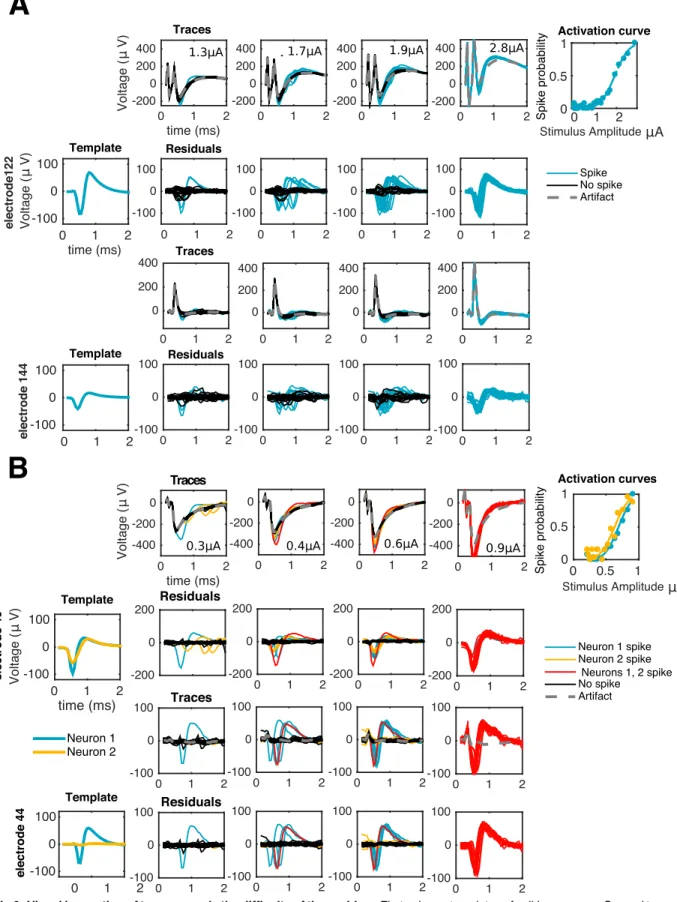
Fig 2. Visual inspection of traces reveals the difficulty of the problem. First column: templates of spiking neurons. Second to

fourth columns: responses of one (A) or two (B) cells to electrical stimulation at increasing stimulation amplitudes as recorded in the stimulating electrode (first rows) or a neighboring, non-stimulating electrode (third rows). If the stimulation artifact is known (gray traces)

(represented by electrode,e), timet, amplitude of stimulusaj, and stimulus repetitioni.

Repeating the same stimulation leads to the same artifact, up to small random fluctuations, and so by averaging several trials these fluctuations can be reduced, and we can conceive the artifact as a stack of moviesA(e,t,j), one for each amplitude of stimulationaj.

We treat the stimulating and non-stimulating electrodes separately because of their observed different qualitative properties.

Stimulating electrode. Modeling the artifact in the stimulating electrode requires special

care because it is this electrode that typically will capture the strongest neural signal in attempts to directly activate a soma (e.g.Fig 3). The artifact is more complex in the stimulating electrode

it can be subtracted from raw traces to produce a baseline (second and fourth rows) amenable for template matching: traces with spike(s) (colored) match, on each electrode, either a translation of a template (A and B) or the sum of different translations of two or more templates (B). As reflected by the activation curves (fifth column) for strong enough stimuli spiking occurs with probability close to one, consistent with the absence of black traces in the rightmost columns.

https://doi.org/10.1371/journal.pcbi.1005842.g002

Fig 3. Properties of the electrical stimulation artifact revealed by TTX experiments. (A) local, electrode-wise properties of the stimulation artifacts.

Overall, magnitude of the artifact increases with stimulation strength (different shades of blue). However, unlike non-stimulating electrodes, where artifacts have a typical shape of a bump around 0.5 ms (fourth column), the case of the stimulating electrode is more complex: besides the apparent increase in artifact strength, the shape itself is not a simple function of stimulating electrode (first and second rows). Also, for a given stimulating electrode the shape of the artifact is a complex function of the stimulation strength, changing smoothly only within certain stimulation ranges: here, responses to the entire stimulation range are divided into three ranges (first, second, and third column) and although traces within each range look alike, traces from different ranges cannot be guessed from other ranges. (B) stimulation artifacts in a neighborhood of the stimulating electrode, at two different stimulus strengths (left and right). Each trace represents the time course of voltage at a certain electrode. Notice that stimulating electrode (blue) and non-stimulating electrodes (light blue) are plotted in different scales.

[16] and has the following properties here: 1) its magnitude is much greater than that of the non-stimulating electrodes; 2) its effect persists at least 2 ms after the onset of the stimulus; and 3) it is a piece-wise smooth, continuous function of the stimulus strength (Fig 3A). Dis-continuities occur at a pre-defined set of stimulus amplitudes, the “breakpoints” (known beforehand), resulting from gain settings in the stimulation hardware that must change in order to apply stimuli of different magnitude ranges [16]. Notice that these discontinuities are a rather technical and context-dependent feature that may not necessarily apply to all stimula-tion systems, unlike the rest of the properties described here.

Non-stimulating electrodes. The artifact here is much more regular and of lower

magni-tude, and has the following properties (seeFig 3): 1) its magnitude peaks around .4ms follow-ing the stimulus onset, and then rapidly stabilizes; 2) the artifact magnitude typically decays with distance from the stimulating electrode; 3) the magnitude of the artifact increases with increasing stimulus strength.

Based on these observations, we develop a general framework for artifact modeling based on Gaussian processes.

A structured Gaussian process model for stimulation artifacts

From the above discussion we conclude that the artifact is highly non-linear (on each coordi-nate), non-stationary (i.e., the variability depends on the value of each coordicoordi-nate), but struc-tured. The Gaussian process (GP) framework [31] provides powerful and computationally scalable methods for modeling non-linear functions given noisy measurements, and leads to a straightforward implementation of all the usual operations that are relevant for our purposes (e.g. extrapolation and filtering) in terms of some tractable conditional Gaussian distributions.

To better understand the rationale guiding the choice of GPs, consider first a simple Bayesian regression model for the artifact as a noisy linear combination ofBbasis functions Fb(e,t,j) (e.g. polynomials); that is,Aðe;t;jÞ ¼

P_B

b¼1 wbFbðe;t;jÞ þ, with a regularizing

priorp(w) on the weights. Ifp(w) andare modeled as Gaussian, and if we consider the collec-tion ofA(e,t,j) values (over all electrodese, timestepst, and stimulus amplitude indicesj) as one large vectorA, then this translates into an assumption that the vectorAis drawn from a high-dimensional Gaussian distribution. The prior meanμand covarianceKofAcan easily be computed in terms ofFandp(w). Importantly, this simple model provides us with tools to estimate the posterior distribution ofAgiven partial noisy observations (for example, we could estimate the posterior ofAat a certain electrode if we are given its values on the rest of the array). SinceAin this model is a stochastic process (indexed bye,t, andj) with a Gaussian dis-tribution, we say thatAis modeled as a Gaussian process, and writeAGPðm;KÞ.

The main problem with the approach sketched above is that one has to solve some challeng-ing model selection problems: what basis functionsFishould we choose, how large shouldM

be, what parameters should we use for the priorp(w), and so on. We can avoid these issues by instead directly specifying the covarianceKand meanμ(instead of specifyingKandμ indi-rectly, throughp(w),F, etc.).

The parameterμinforms us about the mean behavior of the samples from the GP (here, the average values of the artifact). Briefly, we estimatem^by taking the mean of the recordings at the lowest stimulation amplitude and then subtract off that value from all the traces, so thatμ

can be assumed to be zero in the following. We refer the reader toS1 TextandS1 Figfor details, and stress that all the figures shown in the main text are made after applying this mean-subtraction pre-processing operation.

Next we need to specifyK. This “kernel” can be thought of as a square matrix of size dim(A)× dim(A), where dim(A) is as large asT×E×J*106in our context. This number is

large enough so all elementary operations (e.g. kernel inversion) are prohibitively slow unless further structure is imposed onK—indeed, we need to avoid even storingKin memory, and estimating such a high-dimensional object is impossible without some kind of strong regulari-zation. Thus, instead of specifying every single entry ofKwe need to exploit a simpler, lower-dimensional model that is flexible enough to enforce the qualitative structure onAthat we described in the preceding section.

Specifically, we impose a separable Kronecker product structure onK, leading to tractable and scalable inferences [32,33]. This Kronecker product is defined for any two matrices as (AB)((i1,i2),(j1,j2))=A(i1,j1)B(i2,j2). The key point is that this Kronecker structure allows us to break the huge matrixKinto smaller, more tractable pieces whose properties can be easily specified and matched to the observed data. The result is a much lower-dimensional represen-tation ofKthat serves to strongly regularize our estimate of this very high-dimensional object. InS2 Textwe review the main operations from [34] that enable computational speed-ups due to this Kronecker product representation

We state separate Kronecker decompositions for the non-stimulating and stimulating elec-trodes. For the non-stimulating electrode we assume the following decomposition:

K¼rKtKeKsþ

2

ITEJ; ð2Þ

whereKt,Ke, andKsare the kernels that account for variations in the time, space, and stimulus

magnitude dimensions of the data, respectively. One way to think about the Kronecker prod-uctKtKeKsis as follows: to draw a sample from a GP with mean zero and covariance

KtKeKs, start with an arrayz(t,e,s) filled with independent standard normal random

var-iables, then apply independent linear filters in each directiont,e, andsso that the marginal covariances in each direction correspond toKt,Ke, andKs, respectively. The dimensionless

quantityρis used to control the overall magnitude of variability and the scaled identity matrix

ϕ2Idim(A)is included to allow for slight unstructured deviations from the Kronecker structure.

Notice that we distinguish between this extra prior varianceϕ2and the observation noise vari-anceσ2, associated with the error termofEq 1.

Likewise, for the stimulating electrode we consider the kernel:

K0_¼X R r¼1 rr_Kr t K r sþ 02 ITJ: ð3Þ

Here, the sum goes over the stimulation ranges defined by consecutive breakpoints; and for each of those ranges, the kernelKr

s has non-zero off-diagonal entries only for the stimulation

values within ther-th range between breakpoints. In this way, we ensure artifact information is not shared for stimulus amplitudes across breakpoints. Finally,ρ0_andϕ0_{play a similar role}

as inEq 2.

Now that this structured kernel has been stated it remains to specify parametric families for the elementary kernelsKt,Ke,Ks,Ktr,K

r

s. We construct these from the Mate´rn family, using

extra parameters to account for the behaviors described in Stimulation artifacts.

A non-stationary family of kernels. We consider the Mate´rn(3/2) kernel, the continuous

version of an autoregressive process of order 2. Its (stationary) covariance is given by

Klðx1;x2Þ ¼Klðd¼ jx1 x2jÞ ¼ ð1þ ffiffiffi

3

p

dlÞexpð pffiffiffi3dlÞ: ð4Þ

The parameterλ>0 represents the (inverse) length-scale and determines how fast correlations decay with distance. We use this kernel as a device for representing smoothness; that is, the property that information is shared across a certain dimension (e.g. time). This property is key to induce reasonable extrapolation and filtering estimators, as required by our method.

Naturally, given our rationale for choosing this kernel, similar results should be expected if the Mate´rn(3/2) was replaced by a similar, stationary smoothing kernel.

We induce non-stationarities by considering the family of unnormalized gamma densities

dα,β():

da;bðxÞ ¼ expð xbÞx a_:

ð5Þ

By an appropriate choice of the pair (α,β)>0 we aim to expressively represent non-stationary ‘bumps’ in variability. The functionsdα,β() are then used to create a family of non-stationary

kernels through the processZα,βZα,β(x) =dα,β(x)Y(x) whereY*GP(0,Kλ). ThusYhere is a

smooth stationary process anddserves to modulate the amplitude ofY.Zα,βis abona fideGP

[35] with the following covariance matrix (Dα,βis a diagonal matrix with entriesdα,β()):

Kðl;a;bÞ ¼Da;bKlDa;b: ð6Þ For the non-stimulating electrodes, we choose all three kernelsKt,Ke,KsasK(λ,α,β) in Eq 6, with separate parametersλ,α,βfor each. For the time kernels we use time andtas the relevant covariate (δinEq 4andxinEq 5). The case of the spatial kernel is more involved: although we want to impose spatial smoothness, we also need to express the non-stationarities that depend on the distance between any electrode and the stimulating electrode. We do so by makingδrepresent the distance between recording electrodes, andxrepresent the distance between stimulating and recording electrodes. Finally, for the stimulus kernel we take stimulus strengthajas the covariate but we only model smoothness through the Mate´rn kernel and not

localization (i.e.α,β= 0).

Finally, for the stimulating electrode we use the same method for constructing the kernels

Kr

t,Ksron each range between breakpoints. We provide a notational summary inTable 1.

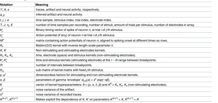
Table 1. Summary of relevant notation.

Notation Meaning

Y, A, s traces, artifact and neural activity, respectively.

^

A,^s inferred artifact and neural activity.

t, j, i, e time sample, stimulus index, trial index, electrode index.

T, J, nj, E number of time samples per recording, number of stimuli, amount of trials per stimulus, number of electrodes in array.

bn

j;i Binary timing vector of spike of neuron n, at trial i of j-th stimulus.

sn

j;i Action potential (if any) of neuron n at trial i of j-th stimulus.

Mn matrix containing action potentials of neuron n, aligned to spiking onset at different times as rows. Kλ Mate´rn(3/2) kernel with inverse length-scale parameterλ.

K, K0 _{Non-stimulating and stimulating electrodes kernels.}

Kt, Ke, Ks time, electrode (space) and stimulus kernels (non-stimulating electrodes). Kr

t,Ksr time and stimulus kernels (stimulating electrode) at the r – th range between breakpoints.

R number of intervals between breakpoints. Kj,j sub-matrix of kernel matrix with fixed j-th stimulus.

ρ,ρr _{dimensionless factors for stimulating and non-stimulating electrode kernels.} α,β parameters of gamma ‘envelope’ dα,β(x) = x

α

exp(−xβ).

θ vector of kernel hyperparameters:θ= (ρ,α,λ,β) and Kθ= Kt, Ke, Ks(non-stimulating electrodes).

ϕ2

noise variance of the artifact. σ2 _{noise variance of recorded traces.} K(θ,ϕ2₎

, K(θ,ϕ02₎

Makes explicit the dependence of K, K0_{on parameters K}(θ,ϕ2₎

= K, K(θ,ϕ02₎

= K0

Algorithm

Now we introduce an algorithm for the joint estimation ofAands, based on the GP model for

A. Roughly, the algorithm is divided in two stages: first, the hyperparameters that govern the structure ofAhave to be found. After, given the inferred hyperparameters we perform the actual inference ofA,sgiven these hyperparameters. We base our approach on posterior infer-ence forp(A,s|Y,θ,σ2)/p(Y|s,A,σ2)p(A|θ), where the first factor in the right hand side is the likelihood of the observed dataYgivens,A, and the noise varianceσ2, and the second stands for the noise-free artifact prior;A*GP(0,Kθ). A summary of all the involved operations is shown in pseudo-code in algorithm 1.

Algorithm 1 Spike detection and Artifact cancellation with electrical stimulation

Input: TracesY = (Yj)j = 1, . . ., J, in response to J stimuli.

Output: Estimates of artifact A^ and neural activity ^sn _{for each neuron.}

EIs of N neurons (e.g. obtained in a visual stimulation experiment).

Initialization

1: Estimate2

(artifact noise) and θ. . Hyperparameter estimation,

Eq (7)

2: Also, estimate σ2 (neural noise) from traces.

Artifact/neural activity inference via coordinate ascent and extrapolation 3: for j = 1, . . . J do 4: Estimate A0 j from A[j−1] (A 0 10Þ. . Extrapolation, Eq (11) 5: while some ^sn

j;i change from one iteration to the nextdo . Coordinate

ascent 6: • Estimate^sn

j;i (for each i, n) greedily. . Matching pursuit, Eq (9)

7: until no spike addition increases the likelihood. 8: • Estimate A^j from residuals Yj

P_N

n¼1snj. . Artifact filtering, Eq (10).

9: end while

10: end for

Initialization: Hyperparameter estimation. From Eqs (2,3,4) and6the GP model for

the artifact is completely specified by the hyperparametersθ= (ρ,α,λ,β) andϕ2,ϕ02. The stan-dard approach for estimatingθis to optimize the marginal likelihood of the observed dataY

[31]. However, in this setting computing this marginal likelihood entails summing over all possible spiking patternsswhile simultaneously integrating over the high-dimensional vector

A; exactly computing this large joint sum and integral is computationally intractable. Instead we introduce a simpler approximation that is computationally relatively cheap and quite effec-tive in practice. We simply optimize the (gaussian) likelihood ofA~,

max y logpð ~ Ajy; 2 Þ ¼min y 1 2A~ t_ðKðy;2Þ_Þ 1_~ Aþ1 2logjK ðy;2Þ_{j; ð7Þ}

whereA~is a computationally cheap proxy for the trueA. The notationK(θ,ϕ2)makes explicit the parametric dependence of the kernels in Eqs2and3, i.e.,K(θ,ϕ2)=Kθ+ϕ2IT×E×J

withKθ=ρKtKeKsfor the non-stimulating electrodes (orK(θ,ϕ 02₎ =Kθ+ϕ02 IT×Eand Ky ¼PR_r¼1r r_Kr tK r

s for the stimulating electrode). Due to the Kronecker structure of these

matrices, onceA~is obtained the terms inEq 7can be computed quite tractably, with computa-tional complexityO(d3), withd= max{E,T,J} (max{T,J} in the stimulating-electrode case), instead ofO(dim(A)3), with dim(A) =ETJ, in the case of a general non-structuredK. Thus the Kronecker assumption here leads to computational efficiency gains of several orders of magnitude. See e.g. [33] for a detailed exposition of efficient algorithmic implementations of

all the operations that involve the Kronecker product that we have adopted here; some poten-tial further accelerations are mentioned in the discussion section below.

Now we need to defineA~. The stimulating electrode case is a bit more straightforward: we have found that settingA~to the mean or median ofYacross trials and then solvingEq 7leads to reasonable hyperparameter settings. The reason is that can neglect the effect of neural activ-ity on traces, as the artifactAis much bigger than the effect of spiking activityson this elec-trode, and. We estimate distinct kernelsK0

t,K 0

sfor each stimulating electrode (since from Fig 3Awe see that there is a good deal of heterogeneity across electrodes), and each of the ranges between breakpoints.Fig 4Bshows an example of some kernels estimated following this approach.

For non-stimulating electrodes, the artifactAis more comparable in size to the spiking con-tributionss, and this simple average-over-trials approach was much less successful, explained also by possible corruptions on ‘bad’, broken electrodes which could lead to equally bad hyper-parameters estimates. On the other hand, for non-stimulating electrodes the artifact shape is much more reproducible across electrodes, so some averaging over electrodes should be effec-tive. We found that a sensible and more robust estimate can be obtained by assuming that the effect of the artifact is a function of the position relative to the stimulating electrode. Under that assumption we can estimate the artifact by translating, for each of the stimulating elec-trodes, all the recorded traces as if they had occurred in response to stimulation at the center electrode, and then taking a big average for each electrode. In other words, we estimate

~ Aðe;t;jÞ ¼1 E XE es¼1 1 nj Xn_j i¼1 Yes_{ðe;t;j;iÞ; ð8Þ}

whereYes_{are the traces in response to stimulation on electrodee}

sandeis the index of

elec-trodeeafter a translation of electrodes so thatesis the center electrode. This centered estimate

leads to stable values ofθ, since combining information across many stimulating electrodes serves to average-out stimulating-electrode-specific neural activity and other outliers.

Some implementation details are worth mentioning. First, we do not combine information of all theEstimulating electrodes, but rather take a large-enough random sample to ensure the stability of the estimate. We found that using*15 electrodes is sufficient. Second, as the effect of the artifact is very localized in space, we do not utilize all the electrodes, but consider only the ones that are close enough to the center (here, the 25% closest). This leads to computational speed-ups without sacrificing estimate quality; indeed, using the entire array may lead to sub-optimal performance, since distant electrodes essentially contribute noise to this calculation. Third, we do not estimateϕ2by jointly maximizingEq 7with respect to (θ,ϕ). Instead, to avoid numerical instabilities we estimateϕ2directly as the background noise of the fictitious artifact. This can be easily done before solving the optimization problem, by considering the portions ofAwith the lowest artifact magnitude, e.g. the last few time steps at the lowest ampli-tude of stimulation at electrodes distant from the stimulating electrode.Fig 4Ashows an exam-ple of kernelsKt,Ke, andKsestimated following this approach.

Coordinate ascent. Once the hyperparametersθare known we focus on the posterior

inference forA,sgivenθand observed dataY. The non-convexity of the set over which the binary vectorsbnare defined makes this problem difficult: many local optima exist in practice and, as a result, for global optimization there may not be a better alternative than to look at a huge number of possible cases. We circumvent this cumbersome global optimization by taking a greedy approach, with two main characteristics: first, joint optimization overAandsis addressed with alternating ascent (overAwithsheld fixed, and then overswithAheld fixed). Alternating ascent is a common approach for related methods in neuroscience (e.g. [12,29]),

Fig 4. Examples of learned GP kernels. A Left: inferred kernels Kt, Ke, Ksin the top, center, and bottom rows, respectively. Center: corresponding stationary auto-covariances from the Mate´rn(3/2) kernels (Eq 4). Right: corresponding unnormalized ‘gamma-like’ envelopes dα,β(Eq 5). The inferred quantities are in

where the recordings are modeled as an additive sum of spiking, noise, and other terms. Sec-ond, data is divided in batches corresponding to the same stimulus amplitude, and the analysis for the (j+ 1)-th batch starts only after definite estimates^s½jŠandA^½jŠhave already been

pro-duced ([j] denotes the set {1,. . .,j}). Moreover, this latter estimate of the artifact is used to ini-tialize the estimate forAj+1(intuitively, we borrow strength from lower stimulation amplitudes

to counteract the more challenging effects of artifacts at higher amplitudes). We address each step of the algorithm in turn below. For simplicity, we describe the details only for the non-stimulating electrodes. Treatment of the non-stimulating electrode is almost the same but demands a slightly more careful handling that we defer to Algorithm.

Given the batchYjand an initial artifact estimateA0j we alternate between neural activity

estimation^sjgiven a current artifact estimate, and artifact estimationA^jgiven the current

esti-mate of neural activity. This alternating optimization stops when changes in every^sn

j are

suffi-ciently small, or nonexistent.

Matching pursuit for neural activity inference. Given the current artifact estimateA^jwe

maximize the conditional distribution for neural activitypðsjjYj;A^j;s

2_{Þ ¼}Qnj

i¼1pðsj;ijYj;i;A^j;s

2_Þ,

which corresponds to the following sparse regression problem (the setSembodies our con-straints on spike occurrence and timing):

min bn j;i2S;n¼1;...;N Xnj i¼1 ðYj;i A^jÞ Xn n¼1 Mn_bn j;i 2 : ð9Þ

We seek to find the allocation of spikes that will lead the best match with the residuals

ðYj;i A^jÞ. We follow a standard template-matching-pursuit greedy approach (e.g. [12]) to

locally optimizeEq 9: specifically, for each trial we iteratively search for the best choice of neu-ron/time, then subtract the corresponding neural activity until the proposed updates no longer lead to increases in the likelihood.

Filtering for artifact inference. Given the current estimate of neural activity^sjwe

maxi-mize the posterior distribution of the artifact, that is,maxA_j pðAjjYj;^sj;y;s

2_{Þ, which here leads}

to the posterior mean estimator (again, the overline indicates mean across thenjtrials):

^ Aj ¼EðAjjYj;^sj;y;s 2_; 2 Þ ¼Ky j;j K y;s2 njþ2 j;j 0 @ 1 A 1 ðYj ^sjÞ: ð10Þ

This operation can be understood as the application of a linear filter. Indeed, by appealing to the eigendecomposition ofKðy;s2=njþ2Þ

j;j we see this operator shrinks them-th eigencomponent

of the artifact by a factor ofκm/(κm+σ2/nj+ϕ2) (κmis the m-th eigenvalue ofK ðy;s2_=n

jþ2Þ

j;j ),

exerting its greatest influence whereκmis small. Notice that in the extreme case thatσ2/nj+ϕ2

is very small compared to theκmthenA^j ðYj ^sjÞ, i.e., the filtered artifact converges to the

simple mean of spike-subtracted traces.

agreement with what is observed inFig 3B: first, the shape of temporal term dα,βreflects that the artifact starts

small, then the variance amplitude peaks at*.5 ms, and then decreases rapidly. Likewise, the corresponding spatial dα,βindicates that the artifact variability induced by the stimulation is negligible for electrodes greater

than 700 microns away from the stimulating electrode. B Same as A), but for the stimulating electrode. Only temporal kernels are shown, for two inter-breakpoint ranges (first and second rows, respectively).

Convergence. Remarkably, in practice often only a few (e.g. 3) iterations of coordinate

ascent (neural activity inference and artifact inference) are required to converge to a stable solutionðsn

jÞfn¼1;...Ng. The required number of iterations can vary slightly, depending e.g. on the

number of neurons or the signal-to-noise; i.e., EI strength versus noise variance.

Iteration over batches and artifact extrapolation. The procedure described in Algorithm

is repeated in a loop that iterates through the batches corresponding to different stimulus strengths, from the lowest to the highest. Also, when doingj!j+ 1 an initial estimate for the artifactA0

jþ1is generated by extrapolating from the current, faithful, estimate of the artifact up

to thej-th batch. This extrapolation is easily implemented as the mean of the noise-free poste-rior distribution in this GP setup, that is:

A0 jþ1¼EðAjþ1jA^½jŠy; 2 Þ ¼Ky ðjþ1;½jŠÞðK ðy;2_Þ ð½jŠ;½jŠÞÞ 1_^ A½jŠ: ð11Þ

Importantly, in practice this initial estimate ends up being extremely useful, as in the absence of a good initial estimate, coordinate ascent often leads to poor optima. The very accurate ini-tializations from extrapolation estimates help to avoid these poor local optima.

We note that both for the extrapolation and filtering stages we still profit from the scalabil-ity properties that arise from the Kronecker decomposition. Indeed, the two required opera-tions—inversion of the kernel and the product between that inverse and the vectorized artifact —reduce to elementary operations that only involve the kernelsKe,Kt,Ks[33].

Integrating the stimulating and non-stimulating electrodes. Notice that the same

algo-rithm can be implemented for the stimulating electrode, or for all electrodes simultaneously, by considering equivalent extrapolation, filtering, and matched pursuit operations. The only caveat is that extrapolation across stimulation amplitude breakpoints does not make sense for the stimulating electrode, and therefore, information from the stimulating electrode must not be taken into account at the first amplitude following a breakpoint, at least for the first match-ing pursuit-artifact filtermatch-ing iteration.

Further computational remarks. Note the different computational complexities of

arti-fact related operations (filtering, extrapolation) and neural activity inference: while the former depends (cubically) only onT,E,J, the latter depends (linearly) on the number of trialsnj, the

number of neurons, and the number of electrodes on which each neuron’s EI is significantly nonzero. In the data analyzed here, we found that the fixed computational cost of artifact infer-ence is typically bigger than the per-trial cost of neural activity inferinfer-ence. Therefore, if spike sorting is required for big volumes of data (nj1) it is a sensible choice to avoid unnecessary

artifact-related operations: as artifact estimates are stable after a moderate number of trials (e.g.nj= 50), one could estimate the artifact with that number, subtract that artifact from

traces and perform matching pursuit for the remaining trials. That would also be helpful to avoid unnecessary multiple iterations of the artifact inference—spike inference loop.

Simplifications and extensions

A simplified method. We now describe a way to reduce some of the computations

associ-ated with algorithm 1. This simplified method is based on two observations: first, as discussed above, if many repetitions are available, the sample mean of spike subtracted traces over trials should already provide an accurate artifact estimator, making filtering (Eq 10) superfluous. (Alternatively, one could also consider the more robust median over trials; in the experiments analyzed here we did not find any substantial improvement with the median estimator.) Sec-ond, as artifact changes smoothly across stimulus amplitudes, it is reasonable to use the artifact estimated at conditionjas an initialization for the artifact estimate at the (j+ 1)th amplitude.

Naturally, if two amplitudes are too far apart this estimator breaks down, but if not, it circum-vents the need to appeal toEq 11.

Thus, we propose a simplified method in whichEq 10is replaced by the spike-subtracted mean voltage (i.e. skip the filtering step in line 9 of algorithm 1), andEq 11is replaced by sim-ple ‘naive’ extrapolation (i.e. avoid kernel-based extrapolation in line 5 of algorithm 1 and just initializeA0

jþ1¼A^½jŠ). We can derive this simplified estimator as a limiting special case within

our GP framework: first, avoiding the filtering operator is achieved by neglecting the noise var-iancesσ2andϕ2, as this essentially means that our observations are noise-free; hence, there is no need for smoothing. Also, our naive extrapolation proposal can be obtained using an arti-fact covariance kernel based on Brownian motion inj[36].

Finally, notice that the simplified method does not require a costly initialization (i.e, we can skip the maximization ofEq 7in line 2 of algorithm 1).

Beyond single-electrode stimulation. So far we have focused our attention on single

elec-trode stimulation. A natural question is whether or not our method can be extended to analyze responses to simultaneous stimulation at several electrodes, which is of particular importance for the use of patterned stimulation as a means of achieving selective activation of neurons [28, 37]. One simple approach is to simply restrict attention to experimental designs in which the relative amplitudes of the stimuli delivered on each electrode are held fixed, while we vary the overall amplitude. This reduces to a one-dimensional problem (since we are varying just a sin-gle overall amplitude scalar). We can apply the approach described above with no modifica-tions to this case, just replacing “stimulus amplitude” in the single-electrode setting with “overall amplitude scale” in the multiple-electrode case.

In this work we consider three types of multiple electrode stimulation:Bipolarstimulation,

Local Returnstimulation andArbitrarystimulation patterns. Bipolar stimuli were applied on two neighboring electrodes, and consisted of simultaneous pulses with opposite amplitudes. The purpose was to modulate the direction of the applied electric field [38]. The local return stimulus had the same central electrode current, with simultaneous current waveforms of opposite sign and one sixth amplitude on the six immediately surrounding return electrodes. The purpose of the local return stimulus configuration was to restrict the current spread of the stimulation pulse by using local grounding. More generally, arbitrary stimulation patterns (up to four electrodes) were similarly designed to shape the resulting electric field, and consisted of simultaneous pulses of varied amplitudes.

Results

We start by showing, inFig 5, an example of the estimation of the artifactAand spiking activ-itysfrom single observed trialsY. Here, looking at individual responses to stimulation pro-vides little information about the presence of spikes, even if the EIs are known. Thus, the estimation process relies heavily on the use of shared information across dimensions: in this example, a good estimate of the artifact was obtained by using information from stimulation at lower amplitudes, and from several trials.

Algorithm validation

We validated the algorithm by measuring its performance both on a large dataset with avail-able human-curated spike sorting and with ground-truth simulated data (we avoid the term ground-truth in the real data to acknowledge the possibility that the human makes mistakes).

Comparison to human annotation. The efficacy of the algorithm was first demonstrated

by comparison to human-curated results from the peripheral primate retina. The algorithm was applied to 4,045 sets of traces in response to increasing stimuli. We refer to each of these

sets as anamplitude series. These amplitude series came from the four stimulation categories described in: single-electrode, bipolar, local return, and arbitrary.

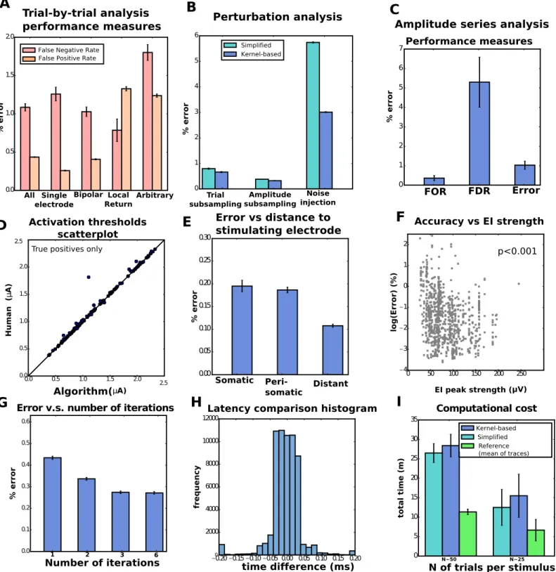
We first assessed the agreement between algorithm and human annotation on a trial-by-trial basis, by comparing the presence or absence of spikes, and their latencies. Results of this trial-by-trial analysis for the kernel-based estimator are shown inFig 6A. Overall, the results are satisfactory, with an error rate of 0.45%. Errors were the result of either false positives (mis-identified spikes over the cases of no spiking) or false negatives (failures in detecting truly existing spikes), whose rates were 0.43% (FPR, false positives over total positives) and 1.08% (FNR, false negatives over total negatives), respectively. For reference, we considered the base-line given by the simple estimator introduced in [20]: there, the artifact is estimated as the sim-ple mean of traces. False negative rates were an order of magnitude larger for the reference estimator, 49% (seeS2 Figfor details). In Comparison to other methods we further discuss why this reference method fails in this data.

We observed comparable error rates for the simplified and kernel-based estimator (again, seeS2 Figfor details). To further investigate differences in performance, we considered three ‘perturbations’ to real data (restricting our attention to single-electrode stimulation, for sim-plicity): sub-sampling of trials (by limiting the maximum number of trials per stimulus to 20, 10, 5, and 2), sub-sampling of amplitudes (considering only every other or every other other stimulus amplitude in the sequence), and noise injection, by adding uncorrelated Gaussian noise with standard deviationσ= 5, 10, or 20μV (this noise adds to the actual noise in record-ings that here we estimated belowσ= 6μV, by using traces in response to low amplitude sti-muli far from the stimulation site). Representative results are shown inFig 6B(but seeS3 Fig for full comparisons), and indicate that indeed the kernel-based estimator delivers superior performance in these more challenging scenarios. Thus unless otherwise noted below we focus on results of the full kernel-based estimator, not the simplified estimator; see Applications: High resolution neural prosthesis for more comparisons between both estimators.

Fig 5. Example of neural activity and artifact inference in a neighborhood of the stimulating electrode. Left: Two recordings in response to a 2.01

μA stimulus. Center: estimated artifact (as the stimulus doesn’t change, it is the same for both trials). Right: Difference between raw traces and estimated artifact, with inferred spikes in color. In the first trial (above) one spiking neuron was detected, while in trial 2 (below) three spiking neurons were detected. The algorithm separates the artifact A and spiking activity s effectively here.

Fig 6. Population results from thirteen retinal preparations reveal the efficacy of the algorithm. A. Trial-by-trial wise performance of estimators

broken down by the the four types of stimulation considered (total number of trials 1,713,233, see Table 1S1 Textfor details). B. Trial-by-trial wise

performance of estimators to perturbations of real data (only single-electrode): five trials per stimulus for trial subsampling, every other stimulus for amplitude subsampling andσ= 20 for noise injection. C,D. Amplitude-series wise performance of estimators. C: false omission rate (FOR = FN/(FN+TP)), false discovery rate (FDR = FP/(FP+TP)), and error rate based on the 4,045 available amplitude series (see Table 2S1 Textfor details); D: comparison of activation thresholds (human vs. kernel-based algorithm). E. Performance measures (trial-by-trial) broken down by distance between neuron and stimulating electrode. F. Trial-by-trial error as a function of EI peak strength across all electrodes (only kernel-based). A Spearman correlation test revealed a significant negative correlation. G. Error as a function of number of iterations in the algorithm. H. For the true positives, histogram of the differences of latencies between

We also quantified accuracy at the level of the entire amplitude series, instead of individual trials: given an amplitude series we conclude that neural activation is present if the sigmoidal activation function fit (specifically, the CDF of a normal distribution) to the empirical activa-tion curves—the proporactiva-tion of trials where spikes occurred as a funcactiva-tion of stimulaactiva-tion amplitude—exceeds 50% within the ranges of stimulation. In the positive cases, we define the stimulation threshold as the current needed to elicit spiking with 0.5 probability. This number provides an informative univariate summary of the activation curve itself. The obtained results are again satisfactory (Fig 6C). Also, in the case of correctly detected events we compared the activation thresholds (Fig 6D) and found little discrepancy between human and algorithm (with the exception of a single point, which can be better considered as an additional false posi-tive, as the algorithm predicts activation at much smaller amplitude of stimulus).

We investigated various covariates that could modulate performance: distance between tar-geted neuron and stimulating electrode (Fig 6E), strength of the neural signals (Fig 6F) and maximum permitted number of iterations of the coordinate ascent step (Fig 6G). Regarding the first, we divided data by somatic stimulation (stimulating electrode is the closest to the soma), peri-somatic stimulation (stimulating electrode neighbors the closest to the soma) and distant stimulation (neither somatic nor peri-somatic). As expected, accuracies were the lowest when the neural soma was close to the stimulating electrode (somatic stimulation), presumably a consequence of artifacts of larger magnitude in that case. Regarding the second, we found that error significantly decreases with strength of the EI, indicating that our algorithm benefits from strong neural signals. With respect to the third, we observe some benefit from increasing the maximum number of iterations, and that accuracies stabilize after a certain value (e.g. three), indicating that either the algorithm converged or that further coordinate iterations did not lead to improvements.

Finally, we report two other relevant metrics: first, differences between real and inferred latencies (Fig 6H, only for correctly identified spikes) revealed that in the vast majority of cases (>95%) spike times inferred by human vs. algorithm differed by less than 0.1 ms. Second, we assessed computational expenses by measuring the algorithm’s running time for the analysis of a single-electrode scan; i.e, the totality of the 512 amplitude series, one for each stimulating electrode (Fig 6I). The analysis was done in parallel, with twenty threads analyzing single amplitude series (details inS1 Text). We conclude that we can analyze a complete experiment in ten to thirty minutes and that the parallel implementation is compatible with the time scales required by closed-loop pipelines. We further comment on this in Online data analysis. Com-parisons inFig 6Ialso illustrate that our methods are 2x-3x slower than the (much less accu-rate) reference estimator, but that differences between kernel-based and the simplified estimator are rather moderate. This suggests that filtering and extrapolation are inexpensive in comparison to the time spent in the matching pursuit stage of the algorithm, and that the cost of finding the hyper-parameters (only once) is negligible at the scale of the analysis of several hundreds of amplitude series.

We refer the reader toS1 Textfor details on population statistics of the analyzed data, exclu-sion criteria, and computational implementation.

Simulations. Synthetic datasets were generated by adding artifacts measured in TTX

recordings (not contaminated by neural activitys), real templates, and white noise, in an attempt to faithfully match basic statistics of neural activity in response to electrical stimuli, i.e., the frequency of spiking and latency distribution as a function of distance between

human and algorithm. I. Computational cost comparison of the three methods for the analysis of single-electrode scans, with 20 to 25 (left) or 50 (right) trials per stimulus.

stimulating electrode and neurons (seeS5 Fig). These simulations (only on single-electrode stimulation) were aimed to further investigate the differences between the naive and kernel-based estimators, by determining when—and to which extent—filtering (Eq 10) and extrapola-tion (Eq 11) were beneficial to enhance performance. To address this question, we evaluated separately the effects of the omission and/or simplification of the filtering operation (Eq 10), and of the replacement of the kernel-based extrapolation (Eq 11) by the naive extrapolation estimator that guesses the artifact at thej-th amplitude of stimulation simply as the artifact at thej− 1 amplitude of stimulation.

As the number of trialsnjgoes to infinity, or as the noise levelσgoes to zero, the influence

of the likelihood grows compared to the GP prior, and the filtering operator converges to the identity (seeEq 10). However, applied on individual traces, where the influence of this opera-tor is maximal, filtering removes high frequency noise components and variations occurring where the localization kernels do not concentrate their mass (Fig 4A), which usually corre-spond to spikes. Therefore, in this case filtering should lead to less spike-contaminated artifact estimates.Fig 7Bconfirms this intuition with results from simulated data: in cases of highσ2

and smallnjthe filtering estimator led to improved results. Moreover, a simplified filter that

only consisted of smoothing kernels (i.e. for all the spatial, temporal and amplitude-wise ker-nels the localization termsdα,βinEq 5were set equal to 1, leading to the Mate´rn kernel in Eq 4) led to more modest improvements, suggesting that the localization terms (Eq 5)—and not only the smoothing kernels—act as sensible and helpful modeling choices.

Likewise, we expect that kernel-based extrapolation leads to improved performance if the artifact magnitude is large compared to the size of the EIs: in this case, differences between the naive estimator and the actual artifact would be large enough that many spikes would be mis-identified or missed. However, since kernel-based extrapolation produces better artifact esti-mates (seeFig 8A and 8B), the occurrence of those failures should be diminished. Indeed, Fig 8Cshows that better results are attained when the size of the artifact is multiplied by a con-stant factor (or equivalently, neglecting the noise termσ2, when the size of the EIs is divided by a constant factor). Moreover, the differential results obtained when including the filtering stage suggest that the two effects are non-redundant: filtering and extrapolation both lead to improvements and the improvements due to each operation are not replaced by the other.

Applications: High resolution neural prosthesis

A prominent application of our method relates to the development of high-resolution neural prostheses (particularly, epi-retinal prosthesis), whose success will rely on the ability to elicit arbitrary patterns of neural activity through the selective activation of individual neurons in real-time [28,39,40]. For achieving such selective activation in a closed-loop setup, we need to know how different stimulating electrodes activate nearby neurons, information that is easily summarized by the activation curves, with the activation thresholds themselves as proxies. Unfortunately, obtaining this information in real time—as required for prosthetic devices—is currently not feasible since estimation of thresholds requires the analysis of individual responses to stimuli. In Online data analysis we discuss in detail how, within our framework, to overcome the stringent time limitations required for such purposes.

Figs9,10,11and12show pictorial representations of different features of the results obtained with the algorithm, and their comparison with human annotation. Axonal recon-structions from all of the neurons in the figures were achieved through a polynomial fit to the neuron’s spatial EI, with soma size depending on the EI strength (see [28] for details). Each of these figures provides particular insights to inform and guide the large-scale closed-loop con-trol of the neural population. Importantly, generation of these maps took only minutes on a

personal computer, compared to many human hours, indicating feasibility for clinical applica-tions and substantial value for analysis of laboratory experiments [28,40].

Fig 9focuses on the stimulating electrode’s point of view: given stimulation in one elec-trode, it is of interest to understand which neurons will get activated within the stimulation range, and how selective that activation can be made. This information is provided by the acti-vation curves, i.e, their steepness and their associated stimulation thresholds. Additionally, latencies can be informative about the spatial arrangement of the system under study, and the mode of neural activation: in this example, one cell is activated through direct stimulation of the soma, and the other, more distant cell is activated through the indirect and antidromic propagation of current through the axon [41]. This is confirmed by the observed latency pattern.

Fig 7. Filtering (Eq 10) leads to a better, less spike-corrupted artifact estimate in our simulations. A effect of filtering on traces for two

non-stimulating electrodes, at a fixed amplitude of stimulation (2.2μA). A1,A3 raw traces, A2,A4 filtered traces. Notice the two main features of the filter: first, it principally affects traces containing spikes, a consequence of the localized nature of the kernel inEq 2. Second, it helps eliminate high-frequency noise. B through simulations, we showed that filtering leads to improved results in challenging situations. Two filters—only smoothing and localization + smoothing—were compared to the omission of filtering. In all cases, to rule out that performance changes were due to the extrapolation estimator, extrapolation was done with the naive estimator. B1 results in a less challenging situation. B2 results in the heavily subsampled (nj= 1) case. B3 results in the high-noise variance (σ2_{= 10) case.}

Fig 10depicts the converse view, focusing on the neuron. Here we aim to determine the cell’s electrical receptive field [37,42] to single-electrode stimulation; that is, the set of elec-trodes that are able to elicit activation, and in the positive cases, the corresponding stimulation thresholds. These fields are crucial for tailoring stimuli that selectively activate sub-populations of neurons.

Fig 11shows how the algorithm enables the analysis of responses to bipolar stimulation. This strategy has been suggested to enhance selectivity [43], by differentially shifting the stimu-lation thresholds of the cells so the range of currents that lead to activation of a single cell is widened. More generally, multi-electrode spatial stimulation patterns have the potential to Fig 8. Kernel-based extrapolation (Eq 11) leads to more accurate initial estimates of the artifact. A comparison between kernel-based extrapolation

and the naive estimator, the artifact at the previous amplitude of stimulation. For a non-stimulating (first row) and the stimulating (second row) electrode, left: artifacts at different stimulus strengths (shades of blue), center: differences with extrapolation estimator (Eq 11), right: differences with the naive estimator. B comparison between the true artifact (black), the naive estimator (blue) and the kernel-based estimator (light blue) for a fixed amplitude of stimulus (3.1μA) on a neighborhood of the stimulating electrode. C Through simulations we showed that extrapolation leads to improved results in a challenging situation. Kernel-based extrapolation was compared to naive extrapolation. C1 results in a less challenging situation. C2-C3 results in the case where the artifact is multiplied by a factor of 3 and 5, respectively.

enhance selectivity by producing an electric field optimized for activating one cell more strongly than others [28], andFig 11is a depiction of how our algorithm permits an accurate assessment of this potential enhancement.

Finally,Fig 12shows a large-scale summary of the responses to single-electrode stimulation. There, a population of ON and OFF parasol cells was stimulated at many different electrodes close to their somas, and each of those cells was then labeled by the lowest achieved activation threshold. These maps provide a proxy of the ability to activate cells with single-electrode stim-ulation, and of the different degrees of difficulty in achieving activation. Since in many cases only as few as 20% of the neurons can be activated [44], the information about which cells were activated can provide a useful guide for the on-line development of more complex multi-ple electrode stimulation patterns that activate the remaining cells.

Discussion

Now we discuss the main features of the algorithm in light of the results and sketch some extensions to enable the analysis of data in contexts that go beyond those analyzed here. Fig 9. Analysis of responses of neurons in a neighborhood of the stimulating electrode. A Spatial configuration:

stimulating electrode (blue/yellow annulus) and four neurons on its vicinity. Soma of green neuron and axon of pink neuron overlap with stimulating electrode. B Activation curves (solid lines) along with human-curated and algorithm inferred spike probabilities (gray and colored circles, respectively) of all the four cells. Stimulation elicited activation of green and pink neurons; however, the two other neurons remained inactive. C Raster plots for the activated cells, with responses sorted by stimulation strength in the y axis. Human and algorithm inferred latencies are in good agreement (gray and colored circles, respectively). Here, direct somatic activation of the green neuron leads to lower-latency and lower-threshold activation than of the pink neuron, which is activated through its axon.

Simplified vs. full kernel-based estimators

Figs6B,7Band8C, andS3 Figillustrate some cases where the full kernel-based estimator out-performs the simplified artifact estimator. These cases correspond to heavy sub-sampling or small signal-to-noise ratios, where the data do not adequately constrain simple estimators of the artifact and the full Bayesian approach can exploit the structure in the problem to obtain significant improvements. In closed-loop experiments (discussed below in Online data analy-sis) experimental time is limited, and the ability to analyze fewer trials without loss of accuracy opens up the possibility for new experimental designs that may not have been otherwise feasible. That said, it is useful to note that simplified estimators are available and accurate in regimes of high SNR and where many trials are available.

Comparison to other methods

We showed that our method strongly outperforms the simple proposal by [20]. Although this competing method was successful on its intended application, here it breaks down since neural activity tends to appear rather deterministically (i.e., spikes occur with very high probability Fig 10. Electrical receptive field of a neuron. A spatial representation of the soma (black circle) and axon (black line) over the array. Electrodes

where stimulation was attempted are represented by circles, with colors indicating the activation threshold in the case of a successful activation of the neuron within the stimulation range. B For those cases, activation curves (solid lines) are shown along with with human and algorithm inferred spike frequencies (gray and colored circles, respectively). Large circles indicate the activation thresholds represented in A. In this case, much of the activity is elicited through axonal stimulation, as there is a single electrode close to the soma that can activate the neuron. Human and algorithm are in good agreement.