Forecasting using a large number of predictors: Is Bayesian regression a valid alternative to principal components?

WO R K I N G PA P E R S E R I E S

N O 7 0 0 / D E C E M B E R 2 0 0 6

FORECASTING USING

A LARGE NUMBER

OF PREDICTORS

IS BAYESIAN

REGRESSION A

VALID ALTERNATIVE

TO PRINCIPAL

COMPONENTS?

In 2006 all ECB publications feature a motif taken from the €5 banknote.

W O R K I N G PA P E R S E R I E S

This paper can be downloaded without charge from http://www.ecb.int or from the Social Science Research Network electronic library at http://ssrn.com/abstract_id=947129

A LARGE NUMBER

OF PREDICTORS

IS BAYESIAN

REGRESSION A

VALID ALTERNATIVE

TO PRINCIPAL

COMPONENTS?

by Christine De Mol

,

Domenico Giannone

and Lucrezia Reichlin

FORECASTING USING

© European Central Bank, 2006 Address

Kaiserstrasse 29

60311 Frankfurt am Main, Germany Postal address

Postfach 16 03 19

60066 Frankfurt am Main, Germany Telephone +49 69 1344 0 Internet http://www.ecb.int Fax +49 69 1344 6000 Telex 411 144 ecb d All rights reserved.

Any reproduction, publication and reprint in the form of a different publication, whether printed or produced electronically, in whole or in part, is permitted only with the explicit written authorisation of the ECB or the

C O N T E N T S

Abstract 4

Non-technical summary 5

1 Introduction 7

2 Three solutions to the “curse of dimensionality”

problem 9

3 Empirics 13

4 Theory 19

5 Conclusions and open questions 22

References 23

6 AppendixA: Proof of proposition 2 25

7 Appendix B 28

8 Appendix C 31

Abstract

This paper considers Bayesian regression with normal and double-exponential priors as forecasting methods based on large panels of time series. We show that, empirically, these forecasts are highly correlated with principal component forecasts and that they perform equally well for a wide range of prior choices. Moreover, we study the asymptotic properties of the Bayesian regression under Gaussian prior under the as-sumption that data are quasi collinear to establish a criterion for setting parameters in a large cross-section.

Keywords: Bayesian VAR, ridge regression, Lasso regression, principal components, large cross-sections

Many problems in economics require the exploitation of large panels of time series. Recent literature has shown the “value” of large information for signal extraction and forecasting and has proposed methods based on factor models to handle the large dimensionality problem (Forni, Hallin, Lippi, and Reich-lin, 2005; Giannone, ReichReich-lin, and Sala, 2004; Stock and Watson, 2002a,b). A related literature has explored the performance of Bayesian model averaging for forecasting (Koop and Potter, 2003; Stock and Watson, 2004, 2005; Wright, 2003) but, surprisingly, few papers explore the performance of Bayesian re-gression in forecasting with high dimensional data. Exceptions are Stock and Watson (2005) who consider normal Bayes estimators for orthonormal regressors and Giacomini and White (2006) who provide an empirical example in which a large Bayesian VAR is compared with principal component regression (PCR).

Bayesian methods are part of the traditional econometrician toolbox and of-fer a natural solution to overcome the curse of dimensionality problem by shrink-ing the parameters via the imposition of priors. In particular, the Bayesian VAR has been advocated as a device for forecasting macroeconomic data (Doan, Lit-terman, and Sims, 1984; LitLit-terman, 1986). It is then surprising that, in most applications, these methods have been applied to relatively small systems and that their empirical and theoretical properties for large panels have not been given more attention by the literature.

This paper is a first step towards filling this gap. We analyze Bayesian regression methods under Gaussian and double-exponential prior.

Our two choices for the prior correspond to two interesting cases: variable aggregation and variable selection. Under Gaussian prior, maximizing the pos-terior distribution generates coefficients (the mode) implying that all variables in the panel are given non-zero coefficients. Regressors, as in PCR are linear combinations of all variables in the panel. The double-exponential, on the other hand, favorssparse models since it puts more mass near zero and in the tails

Non-technical summary

which induces a tendency of the coefficients maximizing the posterior distribu-tion to be either large or zero. As a result, it favors the recovery of a few large coefficients instead of many small ones and truly zero rather than small values. This case is interesting because it results in variable selection rather than in variable aggregation and, in principle, this should give results that are more interpretable from the economic point of view.

For the Gaussian case we show asymptotic results for the size of the cross sectionn and the sample sizeT going to infinity. The analysis provides guid-ance for the the setting of the prior, also interpreted as a Ridge penalization parameter. The empirical analysis reports results for the optimal parameter and for a larger range of parameter choice. The setting of the parameters for the double-exponential case is exclusively empirical. It is designed so as to deliver a given number of non zero coefficients at each estimation step in the out-of-sample evaluation period. The algorithms provide good results by selecting few variables in the regression. We use two algorithms recently proposed which work without limitations of dimensionality: LARS (Least Angle Regression) developed by Efron, Hastie, Johnstone, and Tibshirani (2004) and the Iterative Landweber scheme with soft thresholding at each iteration developed by De Mol and Defrise (2002) and Daubechies, Defrise, and De Mol (2004).

These results show that our data, which correspond to the typical macroe-conomic data-set used for macroemacroe-conomic policy analysis, is characterized by collinearity rather than sparsity. On the other hand, the result that few se-lected variables are able to capture the space spanned by the common factors, suggests that small models with accurately selected variables may do as well as methods that use information on large panels and are based on regressions on linear combinations of all variables. This point calls for further research since our results show that the variable selection provided by the Lasso regression is not clearly interpretable and they are not the typical ones that a macroe-conomist would include in a VAR. Moreover, the selected variables change over time. A conjecture, to be explored in further work, is that, although the under-lying model implies parameter instability, a well chosen approximating model based on a large cross-section has a chance of performing well in forecast since the use of a large number of variables works as a sort of insurance against parameter instability.

1

Introduction

Many problems in economics require the exploitation of large panels of time series. Recent literature has shown the “value” of large information for signal extraction and forecasting and new methods have been proposed to handle the large dimensionality problem (Forni, Hallin, Lippi, and Reichlin, 2005; Gian-none, Reichlin, and Sala, 2004; Stock and Watson, 2002a,b).

A related literature has explored the performance of Bayesian model aver-aging for forecasting (Koop and Potter, 2003; Stock and Watson, 2004, 2005a; Wright, 2003) but, surprisingly, few papers explore the performance of Bayesian regression in forecasting with high dimensional data. Exceptions are Stock and Watson (2005) who consider normal Bayes estimators for orthonormal regressors and Giacomini and White (2006) who provide an empirical example in which a large Bayesian VAR is compared with principal component regression (PCR).

Bayesian methods are part of the traditional econometrician toolbox and of-fer a natural solution to overcome the curse of dimensionality problem by shrink-ing the parameters via the imposition of priors. In particular, the Bayesian VAR has been advocated as a device for forecasting macroeconomic data (Doan, Lit-terman, and Sims, 1984; LitLit-terman, 1986). It is then surprising that, in most applications these methods have been applied to relatively small systems and that their empirical and theoretical properties for large panels have not been given more attention by the literature.

This paper is a first step towards filling this gap. We analyze Bayesian re-gression methods under Gaussian and double-exponential prior and study their forecasting performance on the standard “large” macroeconomic dataset that has been used to establish properties of principal component based forecast (Stock and Watson, 2002a,b). Moreover we analyze the asymptotic properties of Gaussian Bayesian regression for n, the size of the cross-section andT, the sample size, going to infinity. The aim is to establish a connection between Bayesian regression and the classical literature on forecasting with large panels based on principal components.

Our two choices for the prior correspond to two interesting cases: variable aggregation and variable selection. Under Gaussian prior, maximizing the pos-terior distribution generates coefficients (the mode) implying that all variables in the panel are given non-zero coefficients. Regressors, as in PCR are linear combinations of all variables in the panel, but while the Gaussian prior gives de-creasing weight to the ordered eigenvalues of the covariance matrix of the data, principal components imply unit weight to the dominant ones and zero to the others. The double-exponential, on the other hand, favorssparsemodels since it puts more mass near zero and in the tails which induces a tendency of the coefficients maximizing the posterior distribution to be either large or zero. As a result, it favors the recovery of a few large coefficients instead of many small ones and truly zero rather than small values. This case is interesting because it results in variable selection rather than in variable aggregation and, in principle, this should give results that are more interpretable from the economic point of view.

Under double-exponential prior there is no analytical form for the maximizer of the posterior distribution, but we can exploit the fact that, under the prior of i.i.d. regression coefficients, the solution amounts to a Lasso (least absolute shrinkage and selection operator) regression for which there are several algo-rithms. In the empirics we will use two algorithms recently proposed which work without limitations of dimensionality: LARS (Least Angle Regression) developed by Efron, Hastie, Johnstone, and Tibshirani (2004) and the Iterative Landweber scheme with soft thresholding at each iteration developed by De Mol and Defrise (2002) and Daubechies, Defrise, and De Mol (2004).

An interesting feature of the Lasso regression is that it combines variable selection and parameter estimation. The estimator depends on the variable to be predicted and this may have advantages in some empirical situations. The availability of the algorithms mentioned above, which are computationally feasible, makes the double-exponential prior an attractive alternative to other priors used for variable selection such as the one proposed Fernandez, Ley, and Steel (2001) in the contest of Bayesian Model Averaging and applied by Stock and Watson (2005a) for macroeconomic forecasting with large cross-sections, which require computationally demanding algorithms.

Although Gaussian and double-exponential Bayesian regressions imply a dif-ferent form of the forecast equation, an out-of-sample evaluation based on the Stock and Watson dataset, shows that, for a given range of the prior choice, the two methods produce forecasts with similar mean-square errors and which are highly correlated. These forecasts have also similar mean-square errors and are highly correlated with those produced by principal components: they do well when PCR does well. For the case of Lasso, the prior range corresponds to the selection of few variables. However, the forecasts obtained from these informative targeted predictors do not outperform PCR based on few principal components1_.

Since principal component forecasts are known to do well when variables are nearly collinear and this is a typical feature of large panels of macroeconomic data (see Giannone, Reichlin, and Sala, 2004), we study the case of Gaussian regression under near-collinearity and derive conditions on the prior parameters under which the forecast converges to the efficient one (i.e. the forecast under knowledge of the true parameters) asn, the size of the cross-section andT, the sample size, go to infinity.

The technical assumptions under which we derive the result are those that define the approximate factor structure first introduced by Chamberlain and Rothschild (1983) and generalized by Forni and Lippi (2001) and Forni, Hallin, Lippi, and Reichlin (2000). Intuitively, near-collinearity is captured by assuming that, as the size of the cross-sectionnincreases, few eigenvalues increase while the others are bounded. Related assumptions have been introduced by Bai and Ng (2002), Bai (2003), Stock and Watson (2002a) and Stock and Watson

1_{Targeted predictors have recently found to improve performance of factor augmented} forecasts when used to form principal components for factor estimation by Bai and Ng (2006). This result is not directly comparable with ours since we use targeted predictors directly as regressors.

(2002b). Bai (2003), Bai and Ng (2002), Forni, Hallin, Lippi, and Reichlin (2000), Stock and Watson (2002a) and Stock and Watson (2002b) have used them to derive then andT asymptotic properties of the principal component regression.

This result shows how to select the prior in relation to n and helps inter-preting the empirical findings. Under near-collinearity, if the prior is chosen appropriately in relation withn, Bayesian regression under normality will give weight to the principal components associated with the dominant eigenvalues and therefore will produce results which are similar to PCR. But this is what we find in the empirics which indeed shows that our data structure is nearly collinear.

However, our empirics also shows that the same results, similar performances and high correlation with PCR forecasts, are achieved by the Lasso forecast which is based on a regression on few variables. Again, we interpret this re-sult as evidence that our panel is characterized by collinear rather than sparse covariance matrix and that few variables span the space of the pervasive com-mon factors. These variables must be correlated with the principal components. Further work plans to explore this conjecture in more detail.

The paper is organized as follows. The second Section introduces the prob-lem of forecasting using large cross sections. The third Section reports the result of the out-of-sample exercise for the three methods considered: principal com-ponents, Bayesian regression with normal and with double-exponential prior. The fourth Section reports asymptotic results for the (zero mean) Gaussian prior case under approximate factor structure. The fifth Section concludes and outlines problems for future research.

2

Three solutions to the “curse of

dimensional-ity” problem

Consider the (n×1) vector of covariance-stationary processesZt= (z1t, ..., znt)0.

We will assume that they all have mean zero and unitary variance.

We are interested in forecasting linear transformations of some elements of

Ztusing all the variables as predictors. Precisely, we are interested in estimating

the linear projection

yt+h|t= proj{yt+h|Ωt}

where Ωt= span{Zt−p, p= 0,1,2, ...} is a potentially large timet information

set andyt+h=zhi,t+h=fh(L)zi,t+h is a filtered version ofzit, for a specific i.

Traditional time series methods approximate the projection using only a fi-nite number,p, of lags ofZt. In particular, they consider the following regression

model:

yt+h=Zt0β0+...+Zt−p0 βp+ut+h=Xt0β+ut+h

Given a sample of size T, we will denote by X = (Xp+1, ..., XT−h)0 the

(T −h−p)×n(p+ 1) matrix of observations for the predictors and byy = (yp+1+h, ..., yT)0 the (T−h−p)×1 matrix of the observations on the dependent

variable. The regression coefficients are typically estimated by Ordinary Least Squares (OLS), ˆβLS = (X0X)−1X0y, and the forecast is given by ˆyLS_T+h|T =

X_T0βˆLS. When the size of the information set, n, is large, such projection involves the estimation of a large number of parameters. This implies loss of degrees of freedom and poor forecast (“curse of dimensionality problem”). Moreover, if the number of regressors is larger that the sample size,n(p+1)> T, the OLS is not feasible.

To solve this problem, the method that has been considered in the literature is to compute the forecast as a projection on the first few principal components (Forni, Hallin, Lippi, and Reichlin, 2005; Giannone, Reichlin, and Sala, 2004; Giannone, Reichlin, and Small, 2005; Stock and Watson, 2002a,b).

Consider the spectral decomposition of the sample covariance matrix of the regressors:

SxV =V D (1)

where D = diag(d1, ..., dn(p+1)) is a diagonal matrix having on the diagonal

the eigenvalues of Sx = _T−h−p1 X0X in decreasing order of magnitude and

V = (v1, ..., vn(p+1)) is the n(p+ 1)×n(p+ 1) matrix whose columns are the

corresponding eigenvectors2_{. The normalized principal components (PC) are}

defined as: ˆ fit= 1 √ di v0_iXt (2)

fori= 1,· · ·, N whereN is the number of non zero eigenvalues3.

If most of the interactions among the variables in the information set is due to few common underlying factors, while there is limited cross-correlation among the variable specific components of the series, the information content of the large number of predictors can indeed be summarized by few aggregates, while the part not explained by the common factors can be predicted by means of traditional univariate (or low-dimensional forecasting) methods and hence just captured by projecting on the dependent variable itself (or on a small set of predictors). In such situations, few principal components, ˆFt= ( ˆf1t, ...,fˆrt)

withr << n(p+ 1), provide a good approximation of the underlying factors. Assuming for simplicity that lags of the dependent variable are not needed as additional regressors, the principal component forecast is defined as:

y_tP C_+h|t= projyt+h|ΩFt ≈proj{yt+h|Ωt} (3)

2_{The eigenvalues and eigenvectors are typically computed on} 1

T−p PT

t=p+1XtX 0

t (see

for example Stock and Watson, 2002a). We instead compute them on _T−1_h−pX0X = 1

T−p−h PT−h

t=p+1XtX 0

tfor comparability with the other estimators considered in the paper.

where ΩF t = span n ˆ Ft,Fˆt−1,· · ·, o

is a parsimonious representation of the in-formation set. The parsimonious approximation of the inin-formation set makes the projection feasible, since it requires the estimation of a limited number of parameters.

The literature has studied rates of convergence of the principal component forecast to the efficient forecast under assumptions defining an approximate factor structure (see the next Section). Under those assumptions, once common factors are estimated via principal components, the projection is computed by OLS treating the estimated factors as if they were observables.

The Bayesian approach consists instead in imposing limits on the length of

β through priors and estimating the parameters as the posterior mode. The parameters are hence used to compute the forecasts. Here we consider two alternatives: Gaussian and double exponential prior.

Under Gaussian prior, ut ∼ i.i.d. N(0, σu2) and β ∼ N(β0,Φ0), and

as-suming for simplicity that all parameters are shrunk to zero, i.e. β0 = 0, we

have: ˆ βbay= X0X+σu2Φ− 1 0 −1 X0y.

The forecast is hence computed as: ˆ

y_Tbay_+h|T =X_T0 βˆbay.

In the case in which the parameters are independently and identically dis-tributed, Φ0=σβ2I, the estimates are equivalent to those produced by penalized

Ridge regression with parameterν= σ2u

σ2

β

4_{. Precisely}5_:

ˆ

βbay= arg min

β

ky−Xβk2+νkβk2 .

There is a close relation between OLS, PCR and Bayesian regressions. For example, If the prior belief on the regression coefficients is that they are i.i.d., they can be represented as a weighted sum of the projections on the principal components: X_T0βˆ= N X i=1 wifˆiTαˆi (4) where ˆαi = √1_d iv 0

iX0y/(T −h−p) is the regression coefficient ofy on the ith

principal component. For OLS we have wi = 1 for all i. For the Bayesian

4_{Homogenous variance and mean zero are very naive assumptions. In our case, they are} justified by the fact that the variables in the panel we will consider for estimation are stan-dardized and demeaned. This transformation is natural for allowing comparison with principal components.

5_{In what follows we will denote byk · k theL}2 _{matrix norm, i.e. for every matrix A,}

estimates wi = _d di

i+T−νh−p

, where ν = σ2u

σ2

β

. For the PCR regression we have

wi= 1 ifi≤r, and zero otherwise.

OLS, PCR and Gaussian Bayesian regression weight all variables. An alter-native is to select variables. For Bayesian regression, variable selection can be achieved by a double exponential prior, which, when coupled with a zero mean i.i.d. prior, is equivalent to the method that is sometimes called Lasso regression (least absolute shrinkage and selection operator)6_{. In this particular i.i.d. prior}

case the method can also be seen as a penalized regression with a penalty on the coefficients involving theL1 norm instead of theL2 norm. Precisely:

ˆ

βlasso= arg min

β ( ky−Xβk2_+ν n X i=1 |βi| ) (5) where ν = 1_τ where τ is the scale parameter of the prior density7 _{(see e.g.}

Tibshirani, 1996).

Compared with the Gaussian density, the double-exponential puts more mass near zero and in the tails and this induces a tendency to produce estimates of the regression coefficients that are either large or zero. As a result, one favors the recovery of a few large coefficients instead of many fairly small ones. Moreover, as we shall see, the double-exponential prior favors truly zero values instead of small ones, i.e. it favorssparseregression coefficients (sparse mode).

To gain intuition about Lasso regression, let us consider, as an example, the case of orthogonal regressors, a case for which the posterior mode has known analytical form. In particular, let us consider the case in which the regressors are the principal components ofX. In this case, Lasso has the same form of (4) withwiαˆi replaced bySν( ˆαi) whereSν is thesoft-thresholderdefined by

Sν(α) =    α+ν/2 if α≤ −ν/2 0 if |α|< ν/2 α−ν/2 if α≥ν/2. (6)

As seen, this sparse solution is obtained by setting to zero all coefficients ˆαi

which in absolute value lie below the thresholdν/2 and by shrinking the largest ones by an amount equal to the threshold. Let us remark that it would also be possible to leave the largest components untouched, as done in so-called hard-thresholding, but we do not consider this variant here since the lack of continuity of the functionSν(α) makes the theoretical framework more complicated.

In the general case, i.e. with non orthogonal regressors, the Lasso solution will enforce sparsity on the variables themselves rather than on the principal components and this is an interesting feature of the method since it implies a regression on few observables rather than on few linear combinations of the observables. Note that the model with non-Gaussian priors is not invariant under orthogonal linear transformation of the data.

6_{It should be noted however that Lasso is actually the name of an algorithm for finding} the maximizer of the posterior proposed in Tibshirani (1996).

Notice also that, unlike Ridge and PCR, where the selection of the regressors is performed independently of the choice of the series to be forecasted, the Lasso regression depends on that choice.

Methods described by equation (4) will perform well provided that no truly significant coefficientsαiare observed fori > r, because in principal component

regression they will not be taken into account and in Ridge their influence will be highly weakened. Bad performances are to be expected if, for example, we aim at forecasting a time seriesyt, which by bad luck is just equal or close to a

principal component ˆfi withi > r. Lasso solves this problem.

Unfortunately, in the general case the maximizer of the posterior distribution has no analytical form and has to be computed using numerical methods such as the Lasso algortithm of Tibshirani (1996) or quadratic programming based on interior point methods advocated in Chen, Donoho, and Saunders (2001). Two efficient alternatives to the Lasso algorithm, which work without limitations of dimensionality also for sample sizeT smaller than the number of regressors

n(p+ 1), have been developed more recently by Efron, Hastie, Johnstone, and Tibshirani (2004) under the name LARS (Least Angle Regression)8 and by De Mol and Defrise (2002); Daubechies, Defrise, and De Mol (2004) who use instead an Iterative Landweber scheme with soft thresholding at each iteration9. The next section will consider the empirical performance of the three meth-ods discussed in an out-of-sample forecast exercise based on a large panel of time series.

3

Empirics

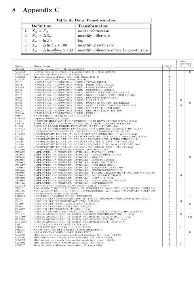
The data set employed for the out-of-sample forecasting analysis is the same as the one used in Stock and Watson (2005b). The panel includes real variables (sectoral industrial production, employment and hours worked), nominal vari-ables (consumer and producer price indices, wages, money aggregates), asset prices (stock prices and exchange rates), the yield curve and surveys. A full description is given in Appendix C.

Series are transformed to obtain stationarity. In general, for real variables, such as employment, industrial production, sales, we take the monthly growth rate. We take first differences for series already expressed in rates: unemploy-ment rate, capacity utilization, interest rate and some surveys. Prices and wages are transformed to first differences of annual inflation following Giannone, Re-ichlin, and Sala (2004); Giannone, ReRe-ichlin, and Small (2005).

Let us define IP as the monthly industrial production index and CPI as the consumer price index. The variables we forecast are

8_{The LARS algorithm has also been used in econometric forecasting by Bai and Ng (2006)} for selecting variables to form principal components in factor augmented forecasts.

9_{The latter algorithm carries out most of the intuition of the orthogonal regression case} and is described in Appendix B. For the LARS algorithm we refer to Efron, Hastie, Johnstone, and Tibshirani (2004).

zh_IP,t+h= (ipt+h−ipt) =zIP,t+h+...+zIP,t+1

and

zhCP I,t+h= (πt+h−πt) =zCP I,t+h+...+zCP I,t+1

whereipt= 100×logIPtis the (rescaled) log of IP andπt= 100×log_{CP I}CP It

t−12

is the annual CPI inflation (IP enters in the pre-transformed panel in first log differences, while annual inflation in first differences).

The forecasts for the (log) IP and the level of inflation are recovered as:

b

ip_T+h|T = ˆz_IP,Th _+h|T +ipT

and

b

πT+h|T = ˆzCP I,Th +h|T+πT

The accuracy of predictions is evaluated using the mean-square forecast error (M SF E) metric, given by:

M SF E_πh= 1 T1−T0−h+ 1 T1−h X T=T0 (_bπT+h|T−πT+h)2 and M SF E_iph = 1 T1−T0−h+ 1 T1−h X T=T0 (ipb_T+h|T −ipT+h)2

The sample has a monthly frequency and ranges from 1959:01 to 2003:12. The evaluation period is 1970:01 to 2002:12. T1=2003:12 is the last available

point in time, T0= 1969:12 and h= 12. We consider rolling estimates with a

window of 10 years, i.e. parameters are estimated at each timeT using the most recent 10 years of data.

All the procedures are applied to standardized data. Mean and variance are re-attributed to the forecasts accordingly.

We report results for industrial production (IP) and the consumer price index (CPI).

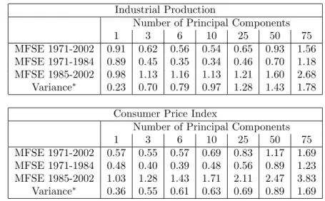
Let us start from principal component regression. We report results for the choice ofr = 1,3,5,10,25,50,75 principal components. The caser = 0 is the forecast implied from a random walk with drift on the log of IP and the annual CPI inflation, whiler=nis the OLS solution. We only report results forp= 0 which is the one typically considered in macroeconomic applications and for which the theory has been developed10 .

We report MSFE relative to the random walk, and the variance of the fore-casts relative to the variance of the series of interest. The MSFE is also reported

10_{The empirical literature has also consider the inclusion of the past of the variable of} interest to capture series specific dynamic. We do not consider this case here since for once few PC are included, series specific dynamics does not help forecasting our variables of interest as shown in D’Agostino and Giannone (2005)

for two sub-samples: the first half of the evaluation period 1970-1985, and the second half 1985-2002. This would help us understand the relative performance of the methods also in a case where the predictability of key macroeconomic time series has dramatically decreased (on this point, see D’Agostino, Giannone, and Surico (2006)). Results are reported in Table 1.

Table 1: Principal component forecasts Industrial Production

Number of Principal Components

1 3 6 10 25 50 75

MFSE 1971-2002 0.91 0.62 0.56 0.54 0.65 0.93 1.56 MFSE 1971-1984 0.89 0.45 0.35 0.34 0.46 0.70 1.18 MFSE 1985-2002 0.98 1.13 1.16 1.13 1.21 1.60 2.68 Variance∗ 0.23 0.70 0.79 0.97 1.28 1.43 1.78

Consumer Price Index

Number of Principal Components

1 3 6 10 25 50 75

MFSE 1971-2002 0.57 0.55 0.57 0.69 0.83 1.17 1.69 MFSE 1971-1984 0.48 0.40 0.39 0.48 0.56 0.89 1.23 MFSE 1985-2002 1.03 1.28 1.43 1.71 2.11 2.47 3.83 Variance∗ 0.36 0.55 0.61 0.63 0.69 0.89 1.69 MSFE are relative to a the Naive, Random Walk, forecast.∗_{The variance of the forecast}

relative to the variance of the series.

Let us start from the whole evaluation sample. Results show that principal components improve a lot over the random walk both for IP and CPI. The advantage is lost when taking too many PC, which implies loss of parsimony. Notice that, as the number of PC increases, the variance of the forecasts becomes larger to the point of becoming larger than the variance of the series itself. This is explained by the large sample uncertainty of the regression coefficients when there is a large number of regressors. Looking at the two sub-samples, we see that PCs perform very well in the first part of the sample, while in the most recent period they perform very poorly, worse than the random walk.

For comparability, we focus on the casep= 0 also for the Bayesian regression (no lags of the regressor). Note, that, for h = 1, this case corresponds to a row of a VAR of order one. The exercise is for the i.i.d. Gaussian prior (Ridge regression). This prior works well for the p= 0 case considered here. However, for the casep >0, it might be useful to shrink more the coefficients of additional lagged regressors, as, for example, with the Minnesota prior (Doan, Litterman, and Sims, 1984; Litterman, 1986). This is beyond the scope of the present empirical analysis which is meant as a first assessment of the general

performance of the methods11.

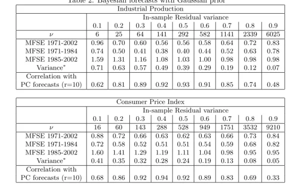
For the Bayesian (Ridge) case, we run the regression using the first estima-tion sample 1959-1969 for a grid of priors. We then choose the priors for which the in-sample fit explains a given fraction 1−κof the variance of the variable to be forecast. We report results for different values ofκ(the associatedν, which are kept fixed for the whole out-of-sample evaluation period, are also reported). Notice that κ= 1 corresponds to the random walk since, in this case, all co-efficients are set to zero. The other extreme,κclose to 0, is associated with a quite uninformative prior and hence will be very close to the OLS. Results are reported in Table 2.

Table 2: Bayesian forecasts with Gaussian prior

Industrial Production

In-sample Residual variance

0.1 0.2 0.3 0.4 0.5 0.6 0.7 0.8 0.9 ν 6 25 64 141 292 582 1141 2339 6025 MFSE 1971-2002 0.96 0.70 0.60 0.56 0.56 0.58 0.64 0.72 0.83 MFSE 1971-1984 0.74 0.50 0.41 0.38 0.40 0.44 0.52 0.63 0.78 MFSE 1985-2002 1.59 1.31 1.16 1.08 1.03 1.00 0.98 0.98 0.98 Variance∗ 0.71 0.63 0.57 0.49 0.39 0.29 0.19 0.12 0.07 Correlation with PC forecasts (r=10) 0.62 0.81 0.89 0.92 0.93 0.91 0.85 0.74 0.48 Consumer Price Index

In-sample Residual variance

0.1 0.2 0.3 0.4 0.5 0.6 0.7 0.8 0.9 ν 16 60 143 288 528 949 1751 3532 9210 MFSE 1971-2002 0.88 0.72 0.66 0.63 0.62 0.63 0.66 0.73 0.84 MFSE 1971-1984 0.72 0.58 0.52 0.51 0.51 0.54 0.59 0.68 0.82 MFSE 1985-2002 1.60 1.41 1.29 1.19 1.11 1.04 0.98 0.95 0.95 Variance∗ 0.41 0.35 0.32 0.28 0.24 0.19 0.13 0.08 0.05 Correlation with PC forecasts (r=10) 0.68 0.86 0.92 0.94 0.92 0.89 0.83 0.69 0.33 MSFE are relative to a the Naive, Random Walk, forecast.∗The variance of the forecast relative to the variance of the series.

The Ridge forecast performs well for a range of κ between 30% and 70% that are associated with shrinkage parameters between half and ten times the cross-sectional dimension,n. For the whole sample, the MSFE are close to that obtained with principal component regression. Moreover, the forecasts produced by Ridge regressions are smoother than the PC forecasts, which is a desirable property.

11_{An additional feature of the Litterman priors is to shrink less coefficients associated with} the variable we are interested in forecasting. This can be helpful when series specific dynamics have significant forecasting power. We do not consider here this case for comparability with the PC case. See Footnote 3.

The last line of the table shows the correlation among Ridge forecasts and principal component forecasts12. Principal components and Ridge forecasts are highly correlated, particularly when the prior is such that the forecasting per-formances are good. The fact that correlation is maximal for parameters giving the best forecasts suggests that there is a common explanation for the good performance of the two methods.

As for the two sub-samples, results are also qualitatively similar to principal component forecasts. Ridge performs particularly well in the first sub-sample but loses all the advantage in the second. We can note, however, more stability than in the principal components case. This is not surprising since Ridge uses all eigenvalues in decreasing importance instead of truncating afterras in the principal components case. Notice also that, for inflation, with ν in the inter-mediate range, even in the most recent sample there is a slight improvement over the random walk.

Finally, we analyze the case of double-exponential priors. In this case, in-stead of fixing the values of the parameterν, we select the prior that delivers a given number (k) of non zero coefficients at each estimation step in the out-of-sample evaluation period. We look at the cases of k = 1,3,5,10,25,50,75 non-zero coefficients13.

Results, reported in Table 3, show that good forecasts are obtained with a limited number of predictors, between 5 and 25. As for Ridge, maximal correlation with the principal component forecast is achieved for the selection of parameters that gives the best results.

Comparable MSFE for the three methods as well as the correlation of the forecast suggest that the covariance of our data are characterized by few domi-nant eigenvalues. In this case, both PC and Ridge, by keeping the largest ones and giving, respectively zero weight and small weight to the others, should per-form similarly. This point will emerge more clearly in next Section on the basis of the asymptotic analysis.

The result for Lasso is less straightforward to interpret since this is a regres-sion on few variables rather than on few aggregates of the variables. The high correlation of the Lasso forecast with the PC forecast implies two things. First, the panel must be characterized by collinearity rather than sparsity and, sec-ond, few variables must span approximately the space of the pervasive common factors.

Again, the correlation of the two Bayesian forecasts with the principal com-ponent forecast, for the priors that ensure good performance, implies that there must be a common explanation for the success of the three methods.

12_{For the principal component forecasts we user= 10. We obtain similar results also for} r= 3,5, i.e. when PC forecasts perform well.

13_{For this exercise we use the LARS algorithm which delivers at once the Lasso solutions for} any given number of non zero coefficients, fork= 1, ..., n. An alternative is to select the prior νthat deliver a given number (k) of non zero coefficients in the initial sample 1959−1970. Then the priorνcan be kept fixed at each estimation step as done for the Ridge case. In this case, we can use the iterated Landweber algorithm with soft thresholding whose input is the priorν rather than the number of non-zero coefficients. This alternative strategy provides qualitatively similar results. They are availabl request.

Table 3: Lasso forecasts Industrial Production

Number of non-zero coefficients

1 3 5 10 25 50 60 MFSE 1971-2002 0.86 0.69 0.64 0.60 0.64 0.77 1.10 MFSE 1971-1984 0.80 0.56 0.50 0.44 0.47 0.58 0.91 MFSE 1985-2002 1.05 1.05 1.05 1.07 1.14 1.32 1.67 Variance∗ 0.07 0.16 0.24 0.40 0.53 0.65 0.79 Correlation with PC forecasts (r=10) 0.05 0.64 0.81 0.85 0.84 0.68 0.44 Consumer Price Index

Number of non-zero coefficients

1 3 5 10 25 50 75 MFSE 1971-2002 0.90 0.76 0.62 0.59 0.68 0.86 1.06 MFSE 1971-1984 0.88 0.70 0.54 0.48 0.52 0.70 0.93 MFSE 1985-2002 1.00 1.04 1.02 1.14 1.44 1.65 1.68 Variance∗ 0.05 0.09 0.18 0.26 0.33 0.39 0.50 Correlation with PC forecasts (r=10) 0.05 0.64 0.81 0.85 0.84 0.68 0.44 MSFE are relative to a the Naive, Random Walk, forecast. ∗The variance of the forecast relative to the variance of the series.

The variables selected for k ≈ 10 at the beginning and at the end of the out-of-sample evaluation period are reported in the last two column of the table describing the database in Appendix C. Two main results emerge. First, only some of the variables selected are those typically included in small-medium size models: the commodity price indexes, the spreads, money aggregates and stock market variables. Some of the selected variables are sectoral (production, labor market and price indicators) or regional (housing). Second, the selection is different at different points in the sample. Only one variable selected at the beginning of the 70s is also picked-up in the most recent period for CPI inflation forecasts. For IP forecasts, no variables are selected in both periods.

We have two conjectures about these results. The fact that variables are not clearly interpretable probably indicates that the panel contains clusters of correlated variables and the procedure selects a particular one, not necessarily the most meaningful from the economic point of view. This implies that variable selection methods are not easily interpretable in this case. The fact that the procedure selects different variables at different points of the sample, implies temporal instability. On the other hands, results also indicate that temporal instability does not affect the relative performance of principal components and Ridge with respect to Lasso. This suggests that principal components and Ridge, by aggregating all variables in the panel, stabilize results providing a sort of insurance against temporal instability. These conjectures will be explored in

4

Theory

We have seen that the Bayesian regression and PCR regression can be seen as ways of stabilizing OLS when data are nearly collinear (sometimes called reg-ularization methods). Large panels of macroeconomic time series are typically highly collinear (Giannone, Reichlin, and Sala, 2004) so that these methods are also appropriate to deal with the “curse of dimensionality” problem.

This observation motivates the assumptions that we will now introduce to define the asymptotic analysis.

A1) Xthas the following representation14:

Xt= ΛFt+ξt

whereFt= (f1t, ..., frt)0, the common factors, is anr-dimensional

station-ary process with covariance matrix EFtFt0 =Ir andξt, the idiosyncratic

components, is ann(p+ 1)-dimensional stationary process with covariance matrix Eξtξt0 = Ψ.

A2) yt+h=γFt+vt+hwhere vt+his orthogonal toFtandξt.

Assumption A1 can be understood as a quasi-collinearity assumption whereby the bulk of cross-correlation is driven by few orthogonal common factors while the idiosyncratic components are allowed to have a limited amount of cross-correlation. The conditions that limit the cross-sectional correlation are given below (condition CR2).

Under assumption A2, if the common factors Ft were observed, we would

have the unfeasible optimal forecast15_:

y∗_t+h|t=γFt

Following Forni, Hallin, Lippi, and Reichlin (2000, 2005); Forni, Giannone, Lippi, and Reichlin (2005), we will impose two sets of conditions, conditions that ensure stationarity (see appendix A) and conditions on the cross-sectional correlation as n increases16. These conditions are a generalization to the dy-namic case of the conditions defining an approximate factor structure given by Chamberlain and Rothschild (1983). Precisely:

14_{Notice that here we define the factor model overX}

t= (Zt0, ...Zt0−p)

0_{while the literature}

typically defines it overZt. It can be seen that ifZt follows an approximate factor structure

defined below, withkcommon factors, then alsoXtfollows an approximate factor structure

withr≤k(p+ 1) common factors.

15_{We are assuming here that common factors are the only source of forecastable dynamics.} We make this assumption for simplicity and since from an empirical point of view series specific dynamics does not help forecasting our variables of interest. See footnote 3.

CR1) 0<lim infn→∞1nλmin(Λ

0_{Λ)<lim sup}

n→∞1nλmax(Λ

0_Λ)<∞

CR2) lim sup_n→∞λmax(Ψ)<∞and lim infn→∞λmin(Ψ)>0

Note thatCR1 implies that as the cross-sectional dimensional increases few eigenvalues of Σx= ΛΛ0+Ψ remain pervasive whileCR2 implies that the others

are asymptotically bounded.

We study now the properties of the Bayesian estimates if the data are gen-erated from an approximate factor structure. Let us first notice that under our assumptions we have Σx= E(XtXt0) = (ΛΛ0+ Ψ) and Σxy= E(Xtyt+h) = Λγ0.

Consequently, the population regression coefficients are given by

β= Σ−_x1Σxy= (ΛΛ0+ Ψ)−1Λγ0= Ψ−1Λ(Λ0Ψ−1Λ +I)−1γ0

Consider now

yt+h|t=Xt0β =FtΛ0Ψ−1Λ(Λ0Ψ−1Λ +I)−1γ0+ξtΨ−1Λ(Λ0Ψ−1Λ +I)−1γ0

.

Under assumptions CR1-2 we have

Λ0Ψ−1Λ(Λ0Ψ−1Λ +I)−1=I+O ₁ n since kΛ0Ψ−1_Λ(Λ0_Ψ−1_{Λ +I)}−1_−Ik=kΛ0_Ψ−1_Λ(Λ0_Ψ−1_{Λ +I)}−1_(Λ0_Ψ−1_Λ)−1_k ≤ k(Λ0Ψ−1_Λ)−1_k2_kΛ0_Ψ−1_{Λk ≤} λmax(Ψ) λmin(Λ0Λ) 2_λ max(Λ0Λ) λmin(Ψ) =O 1 n Moreover,β =O_√1 n since kΨ−1Λ(Λ0Ψ−1Λ +I)−1k ≤ λmax(Ψ) λmin(Λ0Λ) s λmax(Λ0Λ) λmin(Ψ) =O 1 √ n

This implies that:

Eh(ξtβ)2 i =β0Ψβ ≤ kβk2_{kΨk=O 1} n

hence by the Markov’s inequality we have:

ξtβ=Op

₁

√

n

This proves the following result:

Proposition 1Under assumptions A1-2 and CR1-2 we have:

yt+h|t=γFt+O

₁

√

The result above tells us that, under the factor model representation, the projection over the whole dataset Xt and the projection over the unobserved

common factorsFtare asymptotically equivalent forn→ ∞.

In Proposition 1 we assume that the second order moments of the data are known when performing the projection. What if they are estimated? Under the above Assumptions, it has been shown that the forecasts based on the regres-sion on the firstrprincipal components provide consistent estimates fory∗_t+h|t. The Proposition below gives conditions for the shrinkage parameter that allow to obtain consistent forecasts from Bayesian regression under Gaussian priors. We will need the additional Assumption A3 that insures that the elements of the sample covariances of Xt and yt converge uniformly to their population

counterpart, see the Appendix A for details.

Proposition 2Under assumptions A1-2 and CR1-2, if lim infn→∞λmin_kΦ(Φ_0k0) >0

then: X_t0βˆbay =X_t0β+Op ₁ nTkΦ0k +Op n√TkΦ0k as n, T → ∞, provided that 1 nTkΦ0k −1_{→0 and} 1 n√TkΦ0k −1_{→ ∞ asn, T → ∞,}

Proof. See the Appendix.

If coefficients are i.i.d. N(0, σ2

β), then the conditions are satisfied if σβ2 =

1

cnT1/2+δ, where c is an arbitrary positive constant. Hence, we should shrink the single regressors with an asymptotic rate faster than the _n1. With non i.i.d. prior, the condition lim infn→∞λmin_kΦ0(Φk0) > 0 requires that all the regression

coefficients should be shrunk at the same asymptotic rate. Combining Propositions 1 and 2 we obtain:

CorollaryUnder the assumptions A1-2 and CR1-2 and provided the conditions

of Proposition 2 are satisfied, we have

X_t0βˆbay=γFt+Op ₁ √ n +Op ₁ nTkΦ0k +Op n√TkΦ0k asn, T → ∞.

A suitable choice for the prior iskΦ0k= _cnT11/2+δ. In this case we have: ∆nT

X_t0βˆbay−γFt

where ∆nT = min

n√

n, Tδ_{, T}(1 2−δ)

o

and 0 < δ < 1/2. These rates of con-sistency are different from the ones derived for principal components in Forni, Giannone, Lippi, and Reichlin (2005) and, using a different set of assumptions by Bai (2003), and probably can be improved by imposing further assumptions. Proposition 2 tells us that, under the factor structure assumption, the Bayesian regression should use a prior that, as the cross-section dimension increases, shrinks increasingly more all regression coefficients to zero. The reason is that, if the factors are pervasive in the sense of condition CR1, then all variables are informative for the common factors and we should give weight to all of them. Consequently, as the number of predictors increases, the magnitude of each regression coefficient has to decrease.

The intuition of this result is very simple. The factor structure implies that there are few r dominant eigenvalues that diverge faster than the remaining smaller ones as the cross-section dimension increases. The parameter’s prior chosen as above ensures that the effect of the factors associated with the domi-nant eigenvalues is not distorted asymptotically while for the effect of the smaller ones goes to zero asymptotically. Clearly, as mentioned in the empirical Section, if there are few dominant eigenvalues, both Bayesian regression under normality and PCR will only give weight to the principal components associated to the dominant eigenvalues.

5

Conclusions and open questions

This paper has analyzed the properties of Bayesian regression in large panels of time series and compared them to PCR.

We have considered the Gaussian and the double exponential prior and show that they offer a valid alternative to principal components. For the macroeco-nomic panel considered, the forecast they provide is very correlated to that of PCR and implies similar mean-square forecast errors.

This exercise should be understood as rather stylized. For the Bayesian case there is room for improvement, in particular by using developments in BVAR (Doan, Litterman, and Sims, 1984; Litterman, 1986) and related literature.

In the asymptotic analysis we have considered the Gaussian prior case. For that case, we have shownn, T rates of convergence to the efficient forecast under an approximate factor structure. This analysis guides us in the setting of the prior, also interpreted as a Ridge penalization parameter. The empirical analysis reports results for the optimal parameter and for a larger range of parameter choice. The setting of the parameters for the double-exponential case has been exclusively empirical. It is designed so as to deliver a given number of non zero coefficients at each estimation step in the out-of-sample evaluation period. The algorithm provides good results by selecting few variables in the regression.

These results show that our data, which correspond to the typical macroe-conomic data-set used for macroemacroe-conomic policy analysis, is characterized by collinearity rather than sparsity. On the other hand, the result that few se-lected variables are able to capture the space spanned by the common factors,

suggests that small models with accurately selected variables may do as well as methods that use information on large panels and are based on regressions on linear combinations of all variables. This point calls for further research since our results show that the variable selection provided by the Lasso regression is not clearly interpretable and they are not the typical ones that a macroe-conomist would include in a VAR. Moreover, the selected variables change over time. A conjecture, to be explored in further work, is that, although the under-lying model implies parameter instability, a well chosen approximating model based on a large cross-section has a chance of performing well in forecast since the use of a large number of variables works as a sort of insurance against parameter instability.

References

Bai, J. (2003): “Inferential Theory for Factor Models of Large Dimensions,”

Econometrica, 71(1), 135–171.

Bai, J., and S. Ng(2002): “Determining the Number of Factors in

Approxi-mate Factor Models,”Econometrica, 70(1), 191–221.

(2006): “Forecasting Economic Time Series Using Targeted Predic-tors,” Manuscript, University if Michigan.

Chamberlain, G., andM. Rothschild(1983): “Arbitrage, factor structure

and mean-variance analysis in large asset markets.,”Econometrica, 51, 1305– 1324.

Chen, S. S., D. Donoho,andM. Saunders(2001): “Atomic Decomposition by Basis Pursuit,”SIAM Review, 43, 129–159.

D’Agostino, A.,andD. Giannone(2005): “Comparing Alternative

Predic-tors Based on Large-Panel Factor Models,” Manuscript, Universit´e Libre de Bruxelles.

D’Agostino, A., D. Giannone, andP. Surico(2006): “(Un)Predictability

and Macroeconomic Stability,” Working Paper Series 605, European Central Bank.

Daubechies, I., M. Defrise,and C. De Mol(2004): “An iterative thresh-olding algorithm for linear inverse problems with a sparsity constraint,”

Comm. Pure Appl. Math., 57, 1416–1457.

De Mol, C., and M. Defrise (2002): “A note on wavelet-based inversion

methods,” inInverse Problems, Image Analysis and Medical Imaging, ed. by M. Z. Nashed,andO. Scherzer, pp. 85–96. American Mathematical Society.

Doan, T., R. Litterman, and C. A. Sims(1984): “Forecasting and

Condi-tional Projection Using Realistic Prior Distributions,”Econometric Reviews, 3, 1–100.

Efron, B., T. Hastie, I. Johnstone, and R. Tibshirani (2004): “Least angle regression,”Ann. Statist., 32, 407–499.

Fernandez, C., E. Ley,andM. F. J. Steel(2001): “Benchmark priors for Bayesian model averaging,”Journal of Econometrics, 100(2), 381–427.

Forni, M., D. Giannone, M. Lippi,andL. Reichlin(2005): “Opening the

Black Box: Structural Factor Models with large cross-sections,” Manuscript, Universit´e Libre de Bruxelles.

Forni, M., M. Hallin, M. Lippi,andL. Reichlin(2000): “The Generalized

Dynamic Factor Model: identification and estimation,”Review of Economics and Statistics, 82, 540–554.

(2005): “The Generalized Dynamic Factor Model: one-sided estimation and forecasting,” Journal of the American Statistical Association, 100, 830– 840.

Forni, M., and M. Lippi (2001): “The Generalized Dynamic Factor Model: representation theory.,”Econometric Theory, 17, 1113–1141.

Giacomini, R.,andH. White(2006): “Tests of Conditional Predictive

Abil-ity,”Econometrica, forthcoming.

Giannone, D., L. Reichlin,and L. Sala(2004): “Monetary Policy in Real

Time,” inNBER Macroeconomics Annual, ed. by M. Gertler,andK. Rogoff, pp. 161–200. MIT Press.

Giannone, D., L. Reichlin,andD. Small(2005): “Nowcasting GDP and

in-flation: the real-time informational content of macroeconomic data releases,” Finance and Economics Discussion Series 2005-42, Board of Governors of the Federal Reserve System (U.S.).

Koop, G.,andS. Potter(2003): “Forecasting in large macroeconomic panels using Bayesian Model Averaging,” Staff Reports 163, Federal Reserve Bank of New York.

Litterman, R.(1986): “Forecasting With Bayesian Vector Autoregressions – Five Years of Experience,”Journal of Business and Economic Statistics, 4, 25–38.

Stock, J. H., and M. W. Watson (2002a): “Forecasting Using Principal

Components from a Large Number of Predictors,”Journal of the American Statistical Association, 97, 147–162.

(2002b): “Macroeconomic Forecasting Using Diffusion Indexes.,” Jour-nal of Business and Economics Statistics, 20, 147–162.

Stock, J. H., and M. W. Watson (2004): “Forecasting with many

Stock, J. H., and M. W. Watson (2005a): “An Empirical Comparison Of Methods For Forecasting Using Many Predictors,” Manuscript, Prince-ton University.

Stock, J. H.,andM. W. Watson(2005b): “Implications of Dynamic Factor Models for VAR Analysis,” Unpublished manuscript, Princeton University.

Tibshirani, R.(1996): “Regression shrinkage and selection via the lasso,” J.

Royal. Statist. Soc B., 58, 267–288.

Wright, J. H. (2003): “Forecasting U.S. inflation by Bayesian Model

Aver-aging,” International Finance Discussion Papers 780, Board of Governors of the Federal Reserve System (U.S.).

6

Appendix A: Proof of Proposition 2

Denote:

- byytthe generic variable to be forecast asyt=zith

- the covariance matrix of the regressors as Σx= E(xtx0t). The sample

equiva-lent will be denoted bySx=X0X/T. The estimation error will be denote

byEx= Σx−Sx. These matrices are of dimensionn×n.

- the covariance matrix of the regressors and the variable to be predicted as Σxy= E(xty0t+h). The sample equivalent will be denoted bySxy=X0y/T.

The estimation error will be denote byExy= Σxy−Sxy. These matrices

are of dimensionn×1. We assume stationarity.

Moreover, we need the following assumption:

A3) There exists a positive constant K ≤ ∞, such that for all T ∈ N and

i, j∈N

T E[(ex,ij)

2

]< K andT E[(exy,i)2]< K

as T → ∞, whereex,ij denote thei, jth entry ofEx andexy,i denote the

ith entry of Exy. Sufficient conditions can be found in Forni, Giannone,

Lippi, and Reichlin (2005).

Remark 1We can consider here without loss of generality the case of iid prior

on the coefficients and we will denote by ˜ν = σ2u

TkΦ0k the rescaled penalization

the regression in terms of ˜Zt =

Φ1₀/2Zt √

kΦ0k

. Then the resulting regression coeffi-cients, ˜β =pkΦ0kΦ−

1/2

0 β will be iid with prior variance kΦ0k. Moreover the

transformed regressors ˜Zthave the factor representation

˜ Zt= ˜ΛFt+ ˜ξt where ˜Λ = Φ 1/2 0 Λ √ kΦ0k and ˜ξt= Φ1₀/2ξt √ kΦ0k

. The assumption lim infn→∞λmin_kΦ0(Φ_k0) >0

insures that the transformed model still satisfies conditions CR1 and CR2.

Remark 2 In what follows we will prove the proposition for the case p= 0.

The case p > 0 can be analyzed similarly by noticing that if Zt possesses an

approximate factor structure then alsoXt has it.

Defining Σx(˜ν) = Σx+ ˜νIn and the sample equivalent Sx(˜ν) = Sx+ ˜νIn,

we are interested in the properties ofβ(˜ν) and ˆβ(˜ν) which are solutions of the following linear system of equations:

Σx(˜ν)β(˜ν) = Σxy

Sx(˜ν) ˆβ(˜ν) =Sxy

(7) Notice that β(0) =β is the population regression coefficient and ˆβ(0) = ˆβ

is the sample regression coefficient. For ˜ν > 0 we have the Ridge regression coefficients.

Lemma 1Under assumptions CR1-2 we have

kβ(˜ν)k=O ₁ √ n (8) and kβ−β(˜ν)k=Oν n˜ −3/2 asn→ ∞. (9) Proof. We have: kβ(˜ν)k=k(ΛΛ0+ Ψ + ˜νIn)−1Λγ0k ≤ k(ΛΛ0)−1kkΛkkγ0k

which implies (8) by assumption CR1.

On the other hand, recalling thatβ =β(0), we have

β−β(˜ν) = (ΛΛ0+ Ψ)−1−(ΛΛ0+ Ψ + ˜νIn)−1

Λγ0

= (ΛΛ0+ Ψ)−1νI˜ n(ΛΛ0+ Ψ + ˜νIn)−1Λγ0

thanks to the matrix identity

Hence

kβ−β(˜ν)k ≤ν˜kΛΛ0k−2_{kΛk kγ}0_{k=O(˜ν n}−3/2₎

by assumption CR1. Q.E.D.

Whereas for ˜ν = 0 the optimal regression coefficient β provides consistent forecasts, the Ridge parameter ˜ν introduces a bias which tends to zero for large cross-sectional dimensions provided that it does not increase too fast relatively to the cross-sectional dimension n. Let us go now to sample estimates and investigate relations betweenβ(˜ν) and ˆβ(˜ν). We first need the following lemma: Lemma 2 (i) kExk=Op n √ T (ii) kExyk=Op √_n √ T Proof. We have: kExk2≤trace [Ex0Ex] = n X i=1 n X j=1 e2x,ij

Taking expectations, we obtain:

E   n X i=1 n X j=1 e2x,ij  = n X i=1 n X j=1 Ee2x,ij ≤ n 2_K T =O _n2 T We further havekExyk2=P n i=1e 2

xy,i. Taking expectations:

E " n X i=1 e2_xy,i # = n X i=1 E e2_xy,i ≤nK T =O n T

The results follow from the Markov’s inequality. Q.E.D.

Lemma 3Under assumptions A1-3 and CR1-2,

kβˆ(˜ν)−β(˜ν)k=O √_n ˜ ν√T as n, T → ∞

Proof. From (7) we have ˆ

and hence also ˆ

β(˜ν)−β(˜ν) =Sx(˜ν)−1[Sxy−Σxy] +Sx(˜ν)−1Σxy−Σx(˜ν)−1Σxy

Using again the identity (10), we get ˆ

β(˜ν)−β(˜ν) =Sx(˜ν)−1[Sxy−Σxy] +Sx(˜ν)−1[Σx(˜ν)−Sx(˜ν)]Σx(˜ν)−1Σxy

whence

kβˆ(˜ν)−β(˜ν)k ≤ kSx(˜ν)−1k(kSxy−Σxyk+kΣx(˜ν)−Sx(˜ν)k kβ(˜ν)k)

Using Lemma 2, the bound (8) and the fact that kSx(˜ν)−1k ≤ _ν1_˜ , we get the

desired result. Q.E.D.

Summing up, since kXtk = Op(

√

n), Lemma 1 tells us that β(˜ν)0Xt

con-verges to the optimal projectionβ0_X

tif _n˜ν →0 asn, T → ∞. Lemma 3 tells us

that ˆβ(˜ν)0_X

tconverges toβ(˜ν)0Xtif ν_n˜

√

T → ∞as n, T → ∞. If ˜ν meets both conditions we hence obtain a consistent estimate from ˆβ(˜ν)0Xt. The following

lemma combines both estimates (using the triangular inequality):

Lemma 4Under the assumptions A1-3 and CR1-2, if _n˜ν →0 and _n˜ν√T → ∞

asn, T → ∞, then: ˆ β(˜ν)0Xt=β0Xt+Op ˜ ν n +Op n ˜ ν√T as n→ ∞,

A suitable choice for the regularization parameter is ˜ν =α nT−(1

2−δ), where

αis a constant.

The Proposition 2 is now established using Proposition 1, Lemma 4 and the definition of ˜ν.

7

Appendix B

An alternative to matrix inversion for computing regression estimates is provided by iterative methods as, for example, the so-called Landweber iterationwhich was initially developed for solving the normal equations in (7).

To insure convergence the algorithm is applied to regressors with norm smaller than 1. Since our regressors are standardized, this is insured by us-ing the rescaled regressors ˜X = √ 1

n(p+1)(T−h−p)X, and hence estimate the

Starting from the normal equation of the ordinary least squares, we can rewrite it as ˜β = ˜β+ ˜X0y−X˜0X˜β˜ and try to solve it through the successive approximations scheme

˜

β(j+1)= ˜β(j)+ ˜X0y−X˜0X˜β˜(j); j= 0,1, . . . (11) A nice feature of the Landweber iteration is that it can be easily extended to cope with additional constraints or penalties, and in particular those used in Ridge or Lasso regression. As concerns the Lasso functional (5), Daubechies, Defrise, and De Mol (2004) have recently the followingthresholded Landweber iteration

˜

β(j+1)=Sν( ˜β(j)+ ˜X0y−X˜0X˜β˜(j)); j= 0,1, . . . (12)

where the thresholding operator is acting on a vector componentwise by per-forming the soft-thresholding operation defined by (6) and is thus given by

Sν( ˜β) = [Sν( ˜βi)]i=1,···,n; i= 1, . . . , n (13)

This operation enforces the sparsity of the regression coefficients in the sense that all coefficients below the thresholdν/2 are set to zero. The scheme (12) has been proved in Daubechies, Defrise, and De Mol (2004) to converge to a minimizer of the Lasso functional (5). Let us remark that this functional is not strictly convex when the null-space of ˜X is not reduced to zero and therefore the minimizer of (5) is not necessarily unique.

8

Appendix C

Table A: Data Transformation Definition Transformation

1 Xit=Zit no transformation 2 Xit= ∆Zit monthly difference 4 Xit= lnZit log

5 Xit= ∆ lnZit×100 monthly growth rate 6 Xit= ∆ ln Zit

Zit−12 ×100 monthly difference of yearly growth rate

Lasso Selection∗

Code Description Transf. IP CPI

a0m052 Personal income (AR, bil. chain 2000 $) 5

A0M051 Personal income less transfer payments (AR, bil. chain 2000 $) 5 II

A0M224 R Real Consumption (AC) A0m224gmdc 5

A0M057 Manufacturing and trade sales (mil. Chain 1996 $) 5 A0M059 Sales of retail stores (mil. Chain 2000 $) 5 IPS10 INDUSTRIAL PRODUCTION INDEX - TOTAL INDEX 5 IPS11 INDUSTRIAL PRODUCTION INDEX - PRODUCTS, TOTAL 5 IPS299 INDUSTRIAL PRODUCTION INDEX - FINAL PRODUCTS 5 IPS12 INDUSTRIAL PRODUCTION INDEX - CONSUMER GOODS 5 IPS13 INDUSTRIAL PRODUCTION INDEX - DURABLE CONSUMER GOODS 5 IPS18 INDUSTRIAL PRODUCTION INDEX - NONDURABLE CONSUMER GOODS 5 IPS25 INDUSTRIAL PRODUCTION INDEX - BUSINESS EQUIPMENT 5 IPS32 INDUSTRIAL PRODUCTION INDEX - MATERIALS 5 II IPS34 INDUSTRIAL PRODUCTION INDEX - DURABLE GOODS MATERIALS 5 II IPS38 INDUSTRIAL PRODUCTION INDEX - NONDURABLE GOODS MATERIALS 5 II IPS43 INDUSTRIAL PRODUCTION INDEX - MANUFACTURING (SIC) 5 IPS307 INDUSTRIAL PRODUCTION INDEX - RESIDENTIAL UTILITIES 5 IPS306 INDUSTRIAL PRODUCTION INDEX - FUELS 5

PMP NAPM PRODUCTION INDEX (PERCENT) 1

A0m082 Capacity Utilization (Mfg) 2

LHEL INDEX OF HELP-WANTED ADVERTISING IN NEWSPAPERS (1967=100;SA) 2 LHELX EMPLOYMENT: RATIO; HELP-WANTED ADS:NO. UNEMPLOYED CLF 2 LHEM CIVILIAN LABOR FORCE: EMPLOYED, TOTAL (THOUS.,SA) 5 LHNAG CIVILIAN LABOR FORCE: EMPLOYED, NONAGRIC.INDUSTRIES (THOUS.,SA) 5 LHUR UNEMPLOYMENT RATE: ALL WORKERS, 16 YEARS & OVER (%,SA) 2 LHU680 UNEMPLOY.BY DURATION: AVERAGE(MEAN)DURATION IN WEEKS (SA) 2 LHU5 UNEMPLOY.BY DURATION: PERSONS UNEMPL.LESS THAN 5 WKS (THOUS.,SA) 5 LHU14 UNEMPLOY.BY DURATION: PERSONS UNEMPL.5 TO 14 WKS (THOUS.,SA) 5 LHU15 UNEMPLOY.BY DURATION: PERSONS UNEMPL.15 WKS + (THOUS.,SA) 5 LHU26 UNEMPLOY.BY DURATION: PERSONS UNEMPL.15 TO 26 WKS (THOUS.,SA) 5 LHU27 UNEMPLOY.BY DURATION: PERSONS UNEMPL.27 WKS + (THOUS,SA) 5 A0M005 Average weekly initial claims, unemploy. insurance (thous.) 5 CES002 EMPLOYEES ON NONFARM PAYROLLS - TOTAL PRIVATE 5 CES003 EMPLOYEES ON NONFARM PAYROLLS - GOODS-PRODUCING 5

CES006 EMPLOYEES ON NONFARM PAYROLLS - MINING 5 II CES011 EMPLOYEES ON NONFARM PAYROLLS - CONSTRUCTION 5

CES015 EMPLOYEES ON NONFARM PAYROLLS - MANUFACTURING 5 CES017 EMPLOYEES ON NONFARM PAYROLLS - DURABLE GOODS 5 CES033 EMPLOYEES ON NONFARM PAYROLLS - NONDURABLE GOODS 5 CES046 EMPLOYEES ON NONFARM PAYROLLS - SERVICE-PROVIDING 5 CES048 EMPLOYEES ON NONFARM PAYROLLS - TRADE, TRANSPORTATION, AND UTILITIES 5 CES049 EMPLOYEES ON NONFARM PAYROLLS - WHOLESALE TRADE 5 II CES053 EMPLOYEES ON NONFARM PAYROLLS - RETAIL TRADE 5

CES088 EMPLOYEES ON NONFARM PAYROLLS - FINANCIAL ACTIVITIES 5 I I CES140 EMPLOYEES ON NONFARM PAYROLLS - GOVERNMENT 5

A0M048 Employee hours in nonag. establishments (AR, bil. hours) 5 CES151 AVG WEEKLY HOURS OF PROD. OR NONSUPERV. WORKERS ON PRIVATE NONFARM 1 CES155 AVG WEEKLY HOURS OF PROD. OR NONSUPERV. WORKERS ON PRIVATE NONFARM 2

aom001 Average weekly hours, mfg. (hours) 1

PMEMP NAPM EMPLOYMENT INDEX (PERCENT) 1 I

HSFR HOUSING STARTS:NONFARM(1947-58);TOTAL FARM&NONFARM(1959-)(THOUS.,SA 4 HSNE HOUSING STARTS:NORTHEAST (THOUS.U.)S.A. 4 II

HSMW HOUSING STARTS:MIDWEST(THOUS.U.)S.A. 4 II

HSSOU HOUSING STARTS:SOUTH (THOUS.U.)S.A. 4

HSWST HOUSING STARTS:WEST (THOUS.U.)S.A. 4 I

HSBR HOUSING AUTHORIZED: TOTAL NEW PRIV HOUSING UNITS (THOUS.,SAAR) 4 I HSBNE HOUSES AUTHORIZED BY BUILD. PERMITS:NORTHEAST(THOU.U.)S.A 4 II I HSBMW HOUSES AUTHORIZED BY BUILD. PERMITS:MIDWEST(THOU.U.)S.A. 4 I-II HSBSOU HOUSES AUTHORIZED BY BUILD. PERMITS:SOUTH(THOU.U.)S.A. 4 I HSBWST HOUSES AUTHORIZED BY BUILD. PERMITS:WEST(THOU.U.)S.A. 4

PMI PURCHASING MANAGERS’ INDEX (SA) 1

PMNO NAPM NEW ORDERS INDEX (PERCENT) 1 I

PMDEL NAPM VENDOR DELIVERIES INDEX (PERCENT) 1

PMNV NAPM INVENTORIES INDEX (PERCENT) 1 II

A0M008 Mfrs’ new orders, consumer goods and materials (bil. chain 1982 $) 5 A0M007 Mfrs’ new orders, durable goods industries (bil. chain 2000 $) 5 A0M027 Mfrs’ new orders, nondefense capital goods (mil. chain 1982 $) 5 A1M092 Mfrs’ unfilled orders, durable goods indus. (bil. chain 5 I A0M070 Manufacturing and trade inventories (bil. chain 2000 5 I

Lasso Selection∗

Code Description Transf. IP CPI

A0M077 Ratio, mfg. and trade inventories to sales (based on chain 2000 $) 2 FM1 MONEY STOCK: M1(CURR,TRAV.CKS,DEM DEP,OTHER CK’ABLE DEP)(BIL$,SA) 6

FM2 MONEY STOCK:M2(M1+O’NITE RPS,EURO$,GP&BD MMMFS&SAV&SM TIME DEP(BIL$, 6 I FM3 MONEY STOCK: M3(M2+LG TIME DEP,TERM RP’S&INST ONLY MMMFS)(BIL$,SA) 6

FM2DQ MONEY SUPPLY - M2 IN 1996 DOLLARS (BCI) 5 I I FMFBA MONETARY BASE, ADJ FOR RESERVE REQUIREMENT CHANGES(MIL$,SA) 6

FMRRA DEPOSITORY INST RESERVES:TOTAL,ADJ FOR RESERVE REQ CHGS(MIL$,SA) 6 FMRNBA DEPOSITORY INST RESERVES:NONBORROWED,ADJ RES REQ CHGS(MIL$,SA) 6 FCLNQ COMMERCIAL & INDUSTRIAL LOANS OUSTANDING IN 1996 DOLLARS (BCI) 6

FCLBMC WKLY RP LG COM’L BANKS:NET CHANGE COM’L & INDUS LOANS(BIL$,SAAR) 1 II CCINRV CONSUMER CREDIT OUTSTANDING - NONREVOLVING(G19) 6

A0M095 Ratio, consumer installment credit to personal income (pct.) 2 FSPCOM S&P’S COMMON STOCK PRICE INDEX: COMPOSITE (1941-43=10) 5 FSPIN S&P’S COMMON STOCK PRICE INDEX: INDUSTRIALS (1941-43=10) 5 II FSDXP S&P’S COMPOSITE COMMON STOCK: DIVIDEND YIELD (% PER ANNUM) 2 I FSPXE S&P’S COMPOSITE COMMON STOCK: PRICE-EARNINGS RATIO (%,NSA) 5 FYFF INTEREST RATE: FEDERAL FUNDS (EFFECTIVE) (% PER ANNUM,NSA) 2

CP90 Cmmercial Paper Rate (AC) 2

FYGM3 INTEREST RATE: U.S.TREASURY BILLS,SEC MKT,3-MO.(% PER ANN,NSA) 2 FYGM6 INTEREST RATE: U.S.TREASURY BILLS,SEC MKT,6-MO.(% PER ANN,NSA) 2 FYGT1 INTEREST RATE: U.S.TREASURY CONST MATURITIES,1-YR.(% PER ANN,NSA) 2 FYGT5 INTEREST RATE: U.S.TREASURY CONST MATURITIES,5-YR.(% PER ANN,NSA) 2 FYGT10 INTEREST RATE: U.S.TREASURY CONST MATURITIES,10-YR.(% PER ANN,NSA) 2 FYAAAC BOND YIELD: MOODY’S AAA CORPORATE (% PER ANNUM) 2

FYBAAC BOND YIELD: MOODY’S BAA CORPORATE (% PER ANNUM) 2 II

scp90 cp90-fyff 1 II sfygm3 fygm3-fyff 1 I sFYGM6 fygm6-fyff 1 sFYGT1 fygt1-fyff 1 sFYGT5 fygt5-fyff 1 sFYGT10 fygt10-fyff 1 II sFYAAAC fyaaac-fyff 1 sFYBAAC fybaac-fyff 1

EXRUS UNITED STATES;EFFECTIVE EXCHANGE RATE(MERM)(INDEX NO.) 5 EXRSW FOREIGN EXCHANGE RATE: SWITZERLAND (SWISS FRANC PER U.S.$) 5 EXRJAN FOREIGN EXCHANGE RATE: JAPAN (YEN PER U.S.$) 5 EXRUK FOREIGN EXCHANGE RATE: UNITED KINGDOM (CENTS PER POUND) 5 EXRCAN FOREIGN EXCHANGE RATE: CANADA (CANADIAN $ PER U.S.$) 5 PWFSA PRODUCER PRICE INDEX: FINISHED GOODS (82=100,SA) 6 PWFCSA PRODUCER PRICE INDEX:FINISHED CONSUMER GOODS (82=100,SA) 6 PWIMSA PRODUCER PRICE INDEX:INTERMED MAT.SUPPLIES & COMPONENTS(82=100,SA) 6 PWCMSA PRODUCER PRICE INDEX:CRUDE MATERIALS (82=100,SA) 6 PSM99Q INDEX OF SENSITIVE MATERIALS PRICES (1990=100)(BCI-99A) 6 I PMCP NAPM COMMODITY PRICES INDEX (PERCENT) 1 II II

PUNEW CPI-U: ALL ITEMS (82-84=100,SA) 6 I

PU83 CPI-U: APPAREL & UPKEEP (82-84=100,SA) 6

PU84 CPI-U: TRANSPORTATION (82-84=100,SA) 6 I

PU85 CPI-U: MEDICAL CARE (82-84=100,SA) 6 II

PUC CPI-U: COMMODITIES (82-84=100,SA) 6

PUCD CPI-U: DURABLES (82-84=100,SA) 6

PUS CPI-U: SERVICES (82-84=100,SA) 6

PUXF CPI-U: ALL ITEMS LESS FOOD (82-84=100,SA) 6 PUXHS CPI-U: ALL ITEMS LESS SHELTER (82-84=100,SA) 6 PUXM CPI-U: ALL ITEMS LESS MIDICAL CARE (82-84=100,SA) 6

GMDC PCE,IMPL PR DEFL:PCE (1987=100) 6

GMDCD PCE,IMPL PR DEFL:PCE; DURABLES (1987=100) 6 GMDCN PCE,IMPL PR DEFL:PCE; NONDURABLES (1996=100) 6 GMDCS PCE,IMPL PR DEFL:PCE; SERVICES (1987=100) 6

CES275 AVG HOURLY EARNINGS OF PROD. OR NONSUPERV. WORKERS ON PRIVATE NONFARM 6 I CES277 AVG HOURLY EARNINGS OF PROD. OR NONSUPERV WORKERS ON PRIVATE NONFARM 6 II CES278 AVG HOURLY EARNINGS OF PROD. OR NONSUPERV. WORKERS ON PRIVATE NONFARM 6 HHSNTN U. OF MICH. INDEX OF CONSUMER EXPECTATIONS(BCD-83) 2

∗_{We indicate when forecasting IP or CPI, the variable has been selected by Lasso regression}