Same Queries, Different Data: Can we Predict Query Performance?

Same Queries, Different Data: Can we Predict

Runtime Performance?

Adrian Daniel Popescu

_{, Vuk Ercegovac}

_{, Andrey Balmin}

_{, Miguel Branco}

_{, Anastasia Ailamaki}

1_{Ecole Polytechnique F´ed´erale de Lausanne, CH-1015, Lausanne, Switzerland}

2_{IBM Almaden Research Center, San Jose, CA, USA}

Abstract— We consider MapReduce workloads that are

pro-duced by analytics applications. In contrast to ad hoc query workloads, analytics applications are comprised of fixed data

flows that are run over newly arriving data sets or on different

portions of an existing data set. Examples of such workloads include document analysis/indexing, social media analytics, and ETL (Extract Transform Load).

Motivated by these workloads, we propose a technique that predicts the runtime performance for a fixed set of queries running over varying input data sets. Our prediction technique splits each query into several segments where each segment’s performance is estimated using machine learning models. These per-segment estimates are plugged into a global analytical model to predict the overall query runtime. Our approach uses minimal statistics about the input data sets (e.g., tuple size, cardinality), which are complemented with historical information about prior query executions (e.g., execution time).

We analyze the accuracy of predictions for several segment granularities on both standard analytical benchmarks such as TPC-DS [17], and on several real workloads. We obtain less than 25% prediction errors for 90% of predictions.

I. INTRODUCTION

Query performance prediction is a highly desirable feature for both users and resource management (e.g., schedulers). Users and application developers want to know how long is needed to complete execution while automated resource man-agement often seeks accurate runtime estimations to optimize resource provisioning and scheduling in accordance with user contracted Service Level Agreements (SLAs). For instance, FLEX [19] is such an SLA aware scheduler for MapReduce workloads, which requires accurate execution time estimates to produce the optimal schedule.

In the past few years MapReduce [3] has become popular as an infrastructure for large scale data analysis. MapReduce runs on clusters that scale to thousands of commodity nodes by considering availability and fault tolerance as first class concerns. MapReduce is often used for ETL tasks, and in part as an alternative for parallel data processing at large scale. To simplify querying in MapReduce, several high-level, SQL-like languages have been introduced: Hive-QL [16] (Facebook), Pig Latin [12] (Yahoo!), and Jaql [2] (IBM). These systems enable users to express their queries declaratively, and automatically translate them into flows of MapReduce jobs.

In contrast to traditional DBMS, modeling query runtime performance for MapReduce data flows using pure analytical models (as in traditional query optimization) is still an open

problem. One of the main differences, is that MapReduce does not “own” the data or the query runtime operators. The input data is in-situ files whose structure is opaque to the system. Queries, even if written in a high-level language, often contain user defined functions (UDFs) typically written in Java. In this context, modeling the query runtime using learning techniques based on prior query executions is more feasible.

Previous work on runtime prediction, in the context of traditional DBMS [1], [4], [6] or in the context of MapReduce [5], mostly focuses on estimating the runtime performance of similar queries on the same input datasets. Such techniques use a similarity metric to correlate the query of interest, whose runtime is being predicted, with other similar queries from the training set, for which the runtime is known. In our context, analytics applications use fixed data flows that are run at regularly scheduled intervals over newly arriving data sets. Such workloads include document analysis/indexing, social media analytics, and ETL (Extract Transform Load). For such scenarios, traditional approaches in query runtime prediction requirere-trainingon each of the datasets to provide accurate estimates, which is not practical, or runtimes must be extrapolated. In contrast, our approach can accurately model the processing speeds that correspond to various data sets by sampling the input space and building functions that can model processing speed trends rather than assuming them constant.

In this context, we propose a prediction technique which does not require model fitting every time the input data sets change. Typically, several training data sets suffice for fitting a model per query, which can be later used to predict the runtime performance of the query on new data sets. The proposed prediction technique uses a set of minimal statistics about the input data (i.e., tuple size, input cardinality) and historical information about prior query executions (i.e., query logs).

To compute a runtime estimate, our approach combines a set of machine learning models with a global analytical model. Machine learning has powerful mechanisms to extract corre-lations from historical data. Thus, machine learning models are used as building blocks to capture the processing cost and the output cardinalities of each query segment. Then, a global analytical model is used to estimate the query runtime from its segments’ estimates.

A query can be modeled using one segment (coarse-grain) or multiple segments (fine-(coarse-grain). We consider several

options for segmentation since different granularities may be useful for different scenarios. For example, coarse grain

segments are good candidates for dedicated infrastructures

where performance interference and runtime variability is low. In contrast, fine granularity segments are good candidates for shared infrastructures where the dynamics of the system (e.g., slowdown/speed-up) must be captured. For example, such segmentation is used for query progress estimators [10], [11]. Since all of these scenarios are of interest for our workloads, we propose agenericprediction mechanism which can be applied at different segment granularities according to the particular use case.

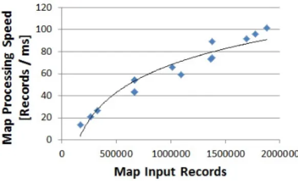
In this paper, we evaluate our proposed prediction technique in the context of applications that were written using Jaql. We investigated correlations between input / output query features including data characteristics and per segment processing costs for several real workloads such as social media analytics, data pre-process for machine learning algorithms, and general analytics (the set of workloads is described in Section III). As a result of the analysis, we found strong correlations between per segment input / output cardinalities, and between input cardinalities / segment processing speeds. Figure 1 and Figure 2 show the observed correlations for a a typical task (pre-process for mining step of social media analytics). We note that, if the observed correlations can be mapped to a function, it is possible to model them either using simple linear regression (i.e., for linear functions) or more specialized regression models such as transform regression [14], which can handle non-linearities in the data (i.e., for more complex functions).

The proposed technique is applicable to MapReduce jobs in general and other high-level languages so long as sufficient information is available in log files to identify traces from similar MapReduce jobs. We note that identifying job types by only comparing job binaries is not robust because additional configuration parameters may be used to decide the actual code fragments executed by the job. For our case, Jaql’s use of transparent functions and their parameters facilitated this task.

In this paper we make the following contributions:

• We propose a technique that predicts the runtime of the

same queries on different input datasets.

• We analyze the sources of errors in predicting query

performance and discuss how prediction errors are prop-agated in our models.

• We evaluate our prediction technique for different levels

of segment granularities and show its feasibility experi-mentally. For the investigated workloads, we obtain less than 25% runtime prediction errors for 90% of predic-tions.

II. PREDICTING THEQUERYRUNTIME

A. Assumptions

First, we assume that the cluster configuration settings are constant. This assumption typically holds in practice if we

consider that the best set of configuration settings is usually chosen at the deployment time per workload rather than per each input query. Second, we assume that data distribution of the inputs does not change. Increasing the table sizes maintains the relative distribution of values constant, i.e. all datasetssample datafrom the same distribution. An important effect of this assumption is data proportionality. I.e., for an input schema, the average record size remains constant. We experimentally validated the last assumption on the work-loads that we investigated, which were typically composed of multiple UDFs that were executed on semi-structured data. However, if the data distribution assumption does not hold for workloads which store data in more traditional, structured format, orthogonal approaches may be employed to build histograms on the columns of interest. For instance, online aggregation techniques as proposed in [13] may be used to build approximate histogramsat a low cost.

B. Approach

We separate queries into query types and we build predic-tion models per query-type as follows. Each query type is defined by the set of MapReduce jobs it requires in the query execution. Further, each MapReduce job is identified by the set of Jaql functions that describe the query semantics of the given job (e. g., filter, aggregate, join, etc). In order to filter the log files of a workload on a particular query-type, we use the following definition of job similarity: two jobs are

considered similar iff all of their Jaql functions are equal.

Such a restrictive definition allows us to use a feature vector consisting of only data processing characteristics instead of a query feature vector that combines query semantics with data processing characteristics.

A typical Jaql query is composed of several MapReduce jobs. A MapReduce job consists of several phases (i.e., the map and reduce phases). In turn, each phase has several processing steps (i.e., read, map, sort, write, shuffle, reduce). In our approach we break the query into several segments and build prediction models at segment granularity. Then, we compute the query runtime using a global model that aggregates each segment’s performance. A segment can be a query, a job, a phase or a processing step according to the level of granularity considered. Figure 3 illustrates phase-level segments.

There was no overhead to collect the data needed to build the models since existing logs were used ’as-is’. The time to build the models for the experiments used in this paper ranged from seconds to minutes, depending the amount of log files analyzed. This overhead and the required disk space needed to store the logs can be tuned as needed by limiting the maximum number of instances stored per job type.

C. Modeling Segment Performance

We use two machine learning models to predict segment performance: a model is used to predict the processing speed of the segment and another model is used to predict the output cardinality of the segment. In constructing these models, we

Fig. 1. Input / output cardinality correlations for Workload-A Fig. 2. Input cardinality / processing speed correlations for Workload-A

Fig. 3. Modeling per segment cardinality functions (i.e.,Ci) and processing

speed functions (i.e.,Pi) for phase-level segments.

use uni-variate linear regression as follows: For predicting the processing speed we use a feature vector (input cardinality,

processing speed), while for predicting the output cardinality

of a segment we use a feature vector(input cardinality, output

cardinality). These models are later used to compute the

runtime estimate of the segment. Using the input cardinality and the processing speed we compute the system utilization time of the segment, while the output cardinality is used as the input into the subsequent segment. For the first segment of the query pipeline we compute the input cardinality based on the input and tuple size of the input datasets.

D. Modeling Query Runtime

To predict the query runtime we combine the performance of each segment on the critical path of the query using a global analytical model. Depending on the level of segment granularity, there are several factors that may need to be considered such as: the level of parallelism (i.e., the number of map / reduce tasks), scheduling overheads, segment overlaps and data skew. In the following we present the methodology for computing the query runtime performance for prediction models that use phase-level segments. This methodology can be easily adapted for other segment granularities (e.g., job, query), and therefore is not presented here.

In order to compute the effective running time of a segment, we divide the system utilization time of the segment by the ac-tual number of tasks used to execute the segment (i.e., multiple tasks are used to increase the degree of parallelism). The actual number of tasks is determined by the cluster configuration, the

job configuration and the amount of input data processed. For instance, the number of map tasks is usually computed based on the size of the input data, while the number of reduce tasks is typically taken from the configuration file.

Given that there are no queuing delays in the system and that the MapReduce cluster is configured such that the reduce phase starts after the map phase finishes, we can use the following formulas to compute the runtime estimate of a query: SegmentRuntime = (T askRuntime+SOtask)×

numW aves, whereT askRuntimeis the average runtime of a map task or a reduce task,SOtaskis the average scheduling overhead per task, and numW aves is the number of waves (i.e., the maximum number of tasks that a worker node is expected to run sequentially) required to execute the job.

The job runtime is computed as follows:

J obRuntime = P_kSegmentRuntimek + SOjob ,

whereSegmentRuntimek is given by the previous formula and the SOjob is the scheduling overhead per job. Currently, all the MapReduce jobs of a given Jaql query are executed sequentially. Therefore, the query runtime estimate is given by adding up the runtime of all MapReduce jobs.

E. Sources of Errors

There are two categories of factors that contribute to inac-curate runtime predictions:

i) Prediction errors caused by non-representative feature vectors or insufficient training at the segment level; in the same category, we also include prediction errors caused by inter-connecting segment models together (i.e., using the pre-dicted output cardinality of one segment as the input of the subsequent segment).

ii) Simplification assumptions about the scheduler (i.e., potential schedules, scheduling overheads), simplification sumptions about data skew and hardware homogeneity as-sumptions across cluster nodes; In order to show how much errors are introduced by the segment level models (case i)) as compared with the errors introduced by simplification assumptions used in the global model (case ii)), we introduce a new metric called theaggregated running time. This metric shows the accuracy of the query runtime that is obtained by composing 100% accurate segment level models. Hence, it exposes the errors introduced by composingthe performance

of segment granularity models into a global runtime estimate (it is effectively measuring the errors introduced by ii)).

We currently account for data skew at the reduce tasks by modeling the skew exposed by earlier job runs on already seen data sets (i.e., we model the performance of the longest reduce task rather than that of the average task). Yet, we omit possible block size differences at the map tasks which may cause additional estimation errors (i.e., we use the average performance of a map task in the global analytical model).

III. EXPERIMENTALSTUDY

We evaluate our prediction techniques on a standard bench-mark on decision support systems and on several real work-loads.

TPC-DS [17]: TPC-DS is a decision support workload modeling a retail supplier. We use TPC-DS because it covers a large variety of decision support queries (e.g., reporting, iterative, data mining) which were designed to cover more realistic scenarios [15] as compared with its precursor (i.e., TPC-H [18]).

Workload-A: Social media data analysis. The categories of queries investigated include: mining process, general pre-process and analytics.

Workload-B: Data pre-processing for machine learning algorithms. The categories of queries include: summarization, cleansing, and statistics computation.

A. Experimental Methodology

Each of the above workloads was run on a dedicated cluster so in this paper, we quantify query prediction accuracy only for this case.

Each time a MapReduce job is evaluated, it outputs a historical file that summarizes how it ran. For Workload-A, we used existing historical files instead of re-executing the queries. For evaluating our models, we used k-fold

cross-validation [7]. Historical files corresponding to each query

were split into k sets where k-1 sets were used for training the models, and 1 set was used for testing the model. For building these sets, we considered only historical files corresponding to query executions ondifferentinput data sets. This process was repeated k times. All prediction errors are computed as the relative error between the predicted and the actual values. We report all prediction errors as cumulative distribution functions.

B. Experimental Setup

We use several different cluster infrastructures. For the TPC-DS benchmark we run our experiments on a 10 node cluster, each of the node having two 6-core CPUs Intel X5660 @ 2.80GHz, 48 GB RAM and 1 Gbps network bandwidth. Workload-A uses a 4 node cluster, while Workload-B uses a 20 node cluster. In all experiments we use Hadoop 0.20.2 configured with FAIR scheduler. The reason for using several infrastructures is that for particular workloads we use existing historical log files from production clusters instead of re-playing all the workloads on the same cluster infrastructure.

C. Job-Level Predictions

We evaluate job-level predictions at multiple segment gran-ularities: i.e., job and phase level. We use 3-level cross-validation to validate our prediction models.

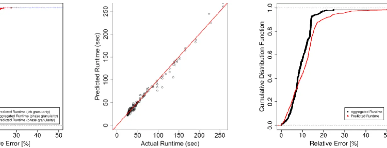
Our first workload consists of a mix of three TPC-DS queries (i.e., Q3, Q7, Q10) and three synthetic queries, all of them using the TPC-DS data. We choose these queries because they include a different number of joins and aggregates, and hence have different complexity (i.e., with query pipelines varying from one single MapReduce job up to a maximum of seven MapReduce jobs). The job runtime varies in the range of [25sec, 4mins]. Figure 4 shows the cumulative distribution function of errors for a total of 186 predictions. For 95% of the workload the prediction errors were less than 20% for all the prediction models analyzed, while job-level models were more accurate, with 10% error for 95% of the workload. The reason that job-level models were more accurate is that they do not require to model the scheduling overheads or the critical path of the query explicitly. The effects of these factors are implicitly included into the features of the job-level models. The small differences between the aggregated runtime and the predicted runtime for phase-level segments show that the main causes that induced a large part of errors for phase-level segments were the simplifying assumptions presented in Section II-E rather than the fine grain models per se.

Figure 5 illustrates the absolute predicted values as com-pared with the actual values for phase-level segments. With a few outliers the predicted values closely match the actual values. This is also illustrated by traditional metrics used in prediction: the coefficient of determination R2_{=0.98 (the} closer to 1, the better), the normalized root-mean-squared

error NRMSE=0.09 (the closer to 0, the better), and the

maximum under-prediction error MUPE=22% (for a job of

136 sec). A full description of these metrics can be found in [7] and a summary in Section 4.2 of [20].

Similar results for Workload A and Workload B are il-lustrated in Figure 6 and Figure 7. These graphs show the prediction errors for phase-level segments only. For Workload A, the job running time varied in the range [16sec, 7.5 hrs], while the job runtime estimation error is less than 15% for 80% of the workload. For Workload B, the job running time varied in the range [1min, 30mins], while the job runtime estimation error is 30% for 80% of the workload. In both cases, our predictions are very close to the aggregated runtime, effectively showing that the prediction models per se have a good accuracy. Similarly, most of the prediction errors were caused by scheduling and critical path approximations.

D. Query-Level Predictions

We evaluated query level predictions at various levels of segment granularities: i.e., query, job and phase levels. We used 3-level cross-validation to validate our prediction models. Figure 8 shows the distribution of prediction errors for the TPC-DS workload. We use the same set of queries as presented in Section III-C. The errors introduced by all prediction schemes was kept under 25% for 90% of the workload.

0 10 20 30 40 50 0.0 0.2 0.4 0.6 0.8 1.0 Relative Error [%] Cum ulativ e Distr ib ution Function ● ● ● ●●●●●●●●●●●●●●●●●●●●●●●●●●●●●●●●●●●●●●●●●●●●●●●●●●●●●●●●●●●●●●●●●●●●●●●●●●●●●●●●●●●●●●●●●●●●●●● ● ●● ● ●●●●●●●●● ●●● ● ● ●

Predicted Runtime (job granularity) Aggregated Runtime (phase granularity) Predicted Runtime (phase granularity)

Fig. 4. Job runtime estimation for TPC-DS Fig. 5. Actual Runtime vs. Predicted Runtime for

TPC-DS 0 10 20 30 40 50 0.0 0.2 0.4 0.6 0.8 1.0 Relative Error [%] Cum ulativ e Distr ib ution Function ● ● ● ●●●●●●●●●●●●●●●●●●●●●●●●●●●●●●●●●●●●●●●●●●●●●●●●●●●●●●●●●●●●●●●●●●●●●●●●●●●●●●●●●●●●●●●●●●●●●●●●●●●●●●●●●●●●●●●●●●●●●●●●●●●●●●●●●●●●●●●●●●●●●●●●●●●●●●●●●●●●●●●●●●●●●●●●●●●●●●●●●●●●●●●●●●●●●●●●●●●●●●●●●●●●●●●●●●●●●●●●●●●●●●●●●●●●●●●●●●●●●●●●●●●●●●●●●●●●●●●●●●●●●●●●●●●●●●●●●●●●●●●●●●●●●●●●●●●●●●●●●●●●●●●●●●●●●●●●●●●●●●●●●●●●●●●●●●●●●●●●●●●●●●●●●●●●●●●●●●●●●●●●●●●●●●●●●●●●●●●●●●●●●●●●●●●●●●●●●●●●●●●●●●●●●●●●●●●●●●●●●●●●●●●●●●●●●●●●●●●●●●●●●●●●●●●●●●●●●●●●●●●●●●●●●●●●●●●●●●●●●●●●●●●●●●●●●●●●●●●●●●●●●●●●●●●●● ●● ● ●Aggregated Runtime Predicted Runtime

Fig. 6. Job runtime estimation for Workload-A

0 20 40 60 80 0.0 0.2 0.4 0.6 0.8 1.0 Relative Error [%] Cum ulativ e Distr ib ution Function ● ● ● ● ●●●●●●●●●● ●●● ●●● ● ●● ● ● ● ●● ● ●●●●●● ●●●● ● ● ●● ●●● ● ●● ●● ● ●●● ● ● ●●●● ● ● ●●●● ● ● ● ●● ●● ● ● ● ●●●●●● ● ● ●● ● ● ●●● ●● ● ● ●Aggregated Runtime Predicted Runtime

Fig. 7. Job runtime estimation for Workload-B

0 10 20 30 40 50 0.0 0.2 0.4 0.6 0.8 1.0 Relative Error [%] Cum ulativ e Distr ib ution Function ● ● ● ● ● ● ● ● ● ● ● ● ● ● ● ● ● ● ● ● ● ● ● ● ●

Predicted Runtime (query granularity) Predicted Runtime (job granularity) Aggregated Runtime (phase granularity) Predicted Runtime (phase granularity)

Fig. 8. Query runtime estimation for TPC-DS

Similarly with job-level predictions, coarse granularity models (i.e., that use query level segments) achieved better accuracy than fine granularity models (i.e., that use job or phase level segments).

Typically, queries with a larger number of MapReduce jobs accumulate more errors than queries with a fewer number of jobs. Yet, an interesting observation is that fine granularity models do not only cumulate errors on the critical path of the query, but may also neutralize cumulated errors if both over- and under- estimations are present. This is one of the reasons that phase granularity models accumulate only 10% more errors than query granularity models for query pipelines composed of up to seven MapReduce jobs.

The total number of predictions is less than for the case of predicting job-level performance because only query-level pre-dictions are reported. For the job-level case, prediction errors for all the jobs of a query were reported. Traditional metrics used in prediction are still in reasonable limits as follows. For phase granularity models: R2_{=0.97, NRMSE=0.25, and}

MUPE=45%, while for query granularity models: R2_=0.99,

the NRMSE=0.07, andMUPE=12%.

In the context of dedicated cluster infrastructures, our tech-nique is more accurate when applied on coarse grain segments

rather than on fine grain segments. This result is not surprising, considering the additional sources of errors for fine granularity models (i.e., scheduling approximations, data skew) and the cumulative errors caused by connecting a larger number of models together. This point is also corroborated by small differences between the predicted runtime and the aggregated runtime, which show the maximum achievable accuracy for fine granularity models. An interesting direction of future work is to combine fine granularity models with coarse granularity models to further improve runtime estimations. The idea is to use the fine granularity models that predict the size and the speed of processing intermediate results and then to use the predicted values as additional inputs in the feature vector of the coarser grain models. Such an approach resembles the models proposed in [21] with the difference that some of the input features of the model are at their turn predicted in a preliminary phase.

IV. RELATEDWORK

Previous work on predicting the runtime execution of MapReduce DAGs was studied from several angles:

Morton et al. propose ParaTimer [11], a progress estimator for MapReduce DAGs. ParaTimer splits each MapReduce job into segments and builds the estimated time left until the

query completes execution using the processing speeds and the input cardinalities of each query segment. Our approach complements ParaTimer as it builds models that predict the cardinality and the processing speed of each query segment.

Herodotou et al. propose Starfish [8], [9], a self-tunning system for Hadoop that aims to find the best set of config-uration settings. Starfish was designed to help practitioners in data analytics getting the best job performance without requiring them knowing the tunning knobs of the underly-ing MapReduce infrastructure. Starfish combines analytical models, simulation and controlled black box models with the goal of finding the best job configuration settings on a given cluster infrastructure. The key building block is thejob profile, which models the processing characteristics of each job. We similarly investigate prior job executions but not only on one representative data set. Instead, for each job type our models

use several reference executions on different data sizes such

that they can approximate processing speed trends (which may change with the input data size). Further, instead of using third party profiling tools, we exploit existing log files produced by Hadoop.

Ganapathi et al. propose an approach for predicting the runtime execution of Hive queries [5]. The proposed approach correlates similar queries using themnearest neighbor queries. However, the proposed model is not designed to predict the runtime performance given that the input datasets change.

V. CONCLUSION ANDFUTUREWORK

In this paper we introduce an approach for predicting the runtime of Jaql queries given that the input datasets change. We propose a hybrid prediction method which combines local linear regression models with a global analytical model. The local models are used to predict per segment performance, while the global analytical model is used to compute the query runtime by aggregating the segment-level estimates. We evaluate and show the feasibility of our approach at various levels of segment granularities on a standard decision support benchmark and on several real workloads.

As ongoing work, we are investigating methods for cor-relating the error causes presented in Section II-E with the actual prediction errors with the goal of providing estimation guarantees. Prediction guarantees are useful to the end users or applications as they may use or disregard an estimation according to the level of guarantee. The challenge sits in providing weights to each error source and to quantify the impact of one error on the other.

We also consider extending our approach such that it can predict the runtime execution when the input data distribution changes. The idea is to introduce the input data distribution as another variable in our prediction models. Specifically, for each attribute of the input data set that is required in the query execution we record its corresponding distribution of values. Prediction models are then built per classes of input distributions (defined by the group of attribute-level distributions). Given a new dataset, our approach will find the model that is closest in terms of its distribution class. For this

purpose, a similarity metric will be defined at the distribution level.

Finally, we plan to evaluate the accuracy of our prediction approach in the context of progress indicators. In particular, we want to study the trade-offs between fine- and coarse-granularity models in the context of shared infrastructures.

ACKNOWLEDGEMENTS

We thank Berthold Reinwald and Robert Metzger for their help with the workloads, and Carl-Christian Kanne for his help with Jaql. We also thank the anonymous reviewers for their constructive feedback on the earlier version of this paper.

REFERENCES

[1] M. Ahmad, S. Duan, A. Aboulnaga, and S. Babu. Interaction-aware

prediction of business intelligence workload completion times. InICDE,

2010.

[2] K. S. Beyer, V. Ercegovac, R. Gemulla, A. Balmin, M. Eltabakh, C.-C. Kanne, F. Ozcan, and E. J. Shekita. Jaql: A Scripting Language for

Large Scale Semistructured Data Analysis. InVLDB, 2011.

[3] J. Dean and S. Ghemawat. MapReduce: Simplified data processing on

large clusters. InOSDI, 2004.

[4] J. Duggan, U. Cetintemel, O. Papaemmanouil, and E. Upfal.

Perfor-mance prediction for concurrent database workloads. InSIGMOD, 2011.

[5] A. Ganapathi, Y. Chen, A. Fox, R. Katz, and D. Patterson.

Statistics-driven Workload Modeling for the Cloud. InICDEW, 2010.

[6] A. Ganapathi, H. Kuno, U. Dayal, J. L. Wiener, A. Fox, M. Jordan, and D. Patterson. Predicting multiple metrics for queries: Better decisions

enabled by machine learning. InICDE, 2009.

[7] T. Hastie, R. Tibshirani, and J. Friedman. The Elements of Statisti-cal Learning: Data Mining, Inference and Prediction, Second Edition. Springer, 2008.

[8] H. Herodotou and S. Babu. Profiling, What-if Analysis, and Cost-based

Optimization of MapReduce Programs. InVLDB, 2011.

[9] H. Herodotou, H. Lim, G. Luo, N. Borisov, L. Dong, F. B. Cetin, and S. Babu. Starfish: A Self-tuning System for Big Data Analytics. In

CIDR, 2011.

[10] G. Luo, J. F. Naughton, and P. S. Yu. Multi-query sql progress indicators.

InEDBT, 2006.

[11] K. Morton, M. Balazinska, and D. Grossman. Paratimer: a progress

indicator for mapreduce dags. InSIGMOD, 2010.

[12] C. Olston, B. Reed, U. Srivastava, R. Kumar, and A. Tomkins. Pig Latin:

A Not-so-foreign Language for Data Processing. InSIGMOD, 2008.

[13] N. Pansare, V. Borkar, C. Jermaine, and T. Condie. Online Aggregation

for Large MapReduce Jobs. InVLDB, 2011.

[14] E. Pednault. Transform Regression and the Kolmogorov Superposition

Theorem. InIBM Research Report RC 23227, IBM Research Division,

2004.

[15] M. Poess, R. O. Nambiar, and D. Walrath. Why You Should Run

TPC-DS: A Workload Analysis. InVLDB.

[16] A. Thusoo, J. S. Sarma, N. Jain, Z. Shao, P. Chakka, S. Anthony, H. Liu, P. Wyckoff, and R. Murthy. Hive: A Warehousing Solution over a

Map-Reduce Framework. Proc. VLDB Endow., 2:1626–1629, 2009.

[17] Transaction Processing Performance Council. TPC Benchmark DS Draft Specification Revision 32. http://www.tpc.org/tpcds.

[18] Transaction Processing Performance Council. TPC Benchmark H

Standard Specification Revision 2.12.0. http://www.tpc.org/tpch. [19] J. Wolf, D. Rajan, K. Hildrum, R. Khandekar, V. Kumar, S. Parekh,

K.-L. Wu, and A. Balmin. FLEX: A Slot Allocation Scheduling Optimizer

for MapReduce Workloads. InMiddleware, 2010.

[20] N. Zhang, P. J. Haas, V. Josifovski, G. M. Lohman, and C. Zhang.

Statistical learning techniques for costing xml queries. InVLDB, pages

289–300, 2005.

[21] Q. Zhu and P.-A. Larson. Building Regression Cost Models for