UCLA
UCLA Electronic Theses and Dissertations
TitleDynamic Word Embedding for News Analysis Permalink https://escholarship.org/uc/item/9tp9g31f Author Zhang, Haoxiang Publication Date 2019 Peer reviewed|Thesis/dissertation
UNIVERSITY OF CALIFORNIA Los Angeles
Dynamic Word Embedding for News Analysis
A thesis submitted in partial satisfaction of the requirements for the degree Master of Science in Computer Science
by
Haoxiang Zhang
c
Copyright by
Haoxiang Zhang 2019
ABSTRACT OF THE THESIS
Dynamic Word Embedding for News Analysis by
Haoxiang Zhang
Master of Science in Computer Science University of California, Los Angeles, 2019
Professor Kai-Wei Chang, Chair
Dynamic word embeddings refer to dividing data into time slices and obtaining the word vector representations of each time slice. By applying dynamic word embeddings, we can analyze how word trends evolve over time. Recently, a number of efforts have been applying dynamic word embeddings to understand how the meanings of words change over years or decades. However, little or no efforts have focused on the monthly changes, which are important for news analysis, such as how a word trend changes monthly. This thesis introduces how to apply dynamic word embeddings for news analysis and presents meaningful word trends evaluations. The application can be extended for news analysis of any time intervals, given enough data within each time slice.
The thesis of Haoxiang Zhang is approved.
Guy Van den Broeck Yizhou Sun Junghoo Cho
Kai-Wei Chang, Committee Chair
University of California, Los Angeles 2019
TABLE OF CONTENTS
1 Introduction . . . 1
2 Word Embeddings . . . 3
2.1 Word2vec . . . 3
2.2 Dynamic Word Embeddings . . . 4
3 Data . . . 6
3.1 2-Month Data Set . . . 6
3.2 6-Month Data Set . . . 6
3.2.1 N gram . . . 7
4 Results . . . 8
4.1 2-month Data Set . . . 8
4.2 6-month Data Set . . . 10
4.2.1 2D Visualization . . . 10
4.2.2 Table . . . 13
4.2.3 Find Changing Words with Absolute Drift . . . 14
5 Discussion . . . 17
LIST OF FIGURES
3.1 Article Count of Each Month (6-month data set) . . . 7
4.1 Shift of the Word ‘Trump’ (2-month data set) . . . 9
4.2 Shift of the Word ‘Croatia’ in 2018 FIFA World Cup (2-month data set) . . . . 10
4.3 Shifts of the Word ‘Stock’ (6-month data set) . . . 11
4.4 Nasdaq Composite Index (6-month) . . . 12
4.5 Shifts of the Word ‘US-Mexico’ (6-month data set) . . . 13
4.6 Shifts of the Word ‘Max’ (6-month data set) . . . 14
4.7 Cosine Similarities with ‘Trad-War’ (6-month data set) . . . 15
4.8 Cosine Similarities with ‘Unemployment’ (6-month data set) . . . 16
LIST OF TABLES
CHAPTER 1
Introduction
Word embeddings are unsupervised learning techniques that map words to vectors. Given large training data sets, these real-valued vectors demonstrate a good semantic
represen-tation. For example, vec(“queen”) will be evaluated as the closest vector to the vector
expressionvec(“man”)−vec(“woman”) +vec(“king”), which encodes the analogy “king is to queen as man is to woman”[PSM14]. Moreover, word embeddings have been used to help a variety of natural language processing (NLP) tasks, such as document classification [Seb02] and sentiment analysis [SPW13].
Recently, a number of efforts have focused on applying dynamic word embeddings to understand how the meanings of words change over time [HLJ16, RB18, BM17, YSD18]. Dynamic word embeddings divide data into time slices and obtain the word vector repre-sentations of each time slice. In their study of historical corpora for English, Hamilton et al.[HLJ16] showed that the word ‘broadcast’ shifts from words like ‘sow’ and ‘seed’ in 1850s to television and radio in 1990s. This means that ‘broadcast’, which referred to “casting out seeds”, developed its meaning of “disseminating information” with the invention of television and radio. In the analysis of 151 years of U.S. Senate speeches, [RB18] identified interesting ways where language changes. For example, subject matter related to Iraq changes from countries like Albania in 1958 to ‘terror’ and ‘terrorism’ in 2008. Although these papers pre-sented interesting results, they focus on the changes of word meanings over years or decades. Little or no efforts have taken up monthly changes in word meanings, which are helpful to analyze news data sets, such as how a topic or word trend changes monthly.
In this thesis, I would like to borrow the technique of dynamic word embedding to study trends in news. For example, the word ‘Trump’ appears in many news articles. During or
immediately after an important event, the word ‘Trump’ may become more relevant to the terms related to this event. When the 2019 North Korea-United States Summit happened in Hanoi, Vietnam, the word ‘Trump’ might have been closely connected to Kim Jung Un (the President of North Korea) and Vietnam (the country that hosted this summit). Another example is that the recent topic of ‘US-Mexico’ news should be mostly related to unau-thorized immigrants across the US-Mexico border, because of President Trump’s election promises. By connecting word vectors from different months with alignment, dynamic word embeddings can capture such trends in news and help the analysis. The rest of this thesis is structured as follows: Chapter 2 describes word embeddings, dynamic word embeddings and how to align word embeddings of different time slices. Chapter 3 explains the dataset, and how to obtain the n-gram or named-entity embeddings. Chapter 4 presents the inter-esting visulization results. Finally, chapter 5 discusses the limitations and potential future directions.
CHAPTER 2
Word Embeddings
Word embeddings represent each word by a low-dimensional vector, while preserving the se-mantic similarities among words. For example, Monday and Tuesday are closer (or have
a higher cosine similarity) than Monday and green. There have been embedding
algo-rithms from 1990s [DDF90, LB96, BDV03]. Recently, word2vec [MCC13, MSC13] and GloVe [PSM14] have been widely used. Word2vec is chosen because [HLJ16] showed its superiority over other embedding methods.
2.1
Word2vec
Word2vec is a model that learns word vectors by maximizing following likelihood [MSF17].
For each word position t, given a fixed window size m predict surrounding context words of
wordwt. L(θ) = T Y t=1 Y −m≤j≤m j6=0 P(wt+j|wt;θ)
Maximizing this likelihood is the same as minimizing following the objective function, which is the average negative log likelihood:
J(θ) =−1 TlogL(θ) =−1 T T X t=1 X −m≤j≤m j6=0 logP(wt+1|wt;θ)
where θ ∈ R2dV represents all model parameters. These parameters are d-dimensional
vectors forV words. Each word w has two vectors:
• uw when it is a context word
For example, for ”...UCLA Centennial Celebration is a year-long series of events...”, take Celebration as the center word wt. Then,P(wt−1|wt) is
P(Centennial|Celebration;uCentennial, vCelebration, θ) If taking Centennial as the center wordwt, then P(wt+1|wt) is
P(Celebration|Centennial;uCelebration, vCentennial, θ)
Let c denote the center word and o denote the context word, then the probability can be
computed as [MSF17] P(o|c) = exp(u T ovc) P w∈V exp(uTwvc) uTv =u·v =Pn
i=1uivi, so the larger dot product u
T
ovc represents larger probability P(o|c) or higher similarity of o and c.
2.2
Dynamic Word Embeddings
Static word embeddings assume that the meaning of any word does not change over time and train the entire corpus by one word embeddings model. For example, it is easy to show that the word ‘trade-war’ has neighboring words such as ‘negotiations’, ‘tensions’ and ‘tariff’, but with a static word embeddings model, it is hard to tell in which month a trade war was tense and in which month it was under gentle negatiations. As another example, static word embeddings can definitely indicate that ‘bullish’ and ‘bearish’ are top neighboring words of the word ‘stock’, but people cannot distinguish when the stock market is bullish or bearish. Dynamic word embeddings can help with these issues.
Unlike the static word embeddings model, the dynamic word embeddings model assumes that word trends do change across time. It divides data into time slices and obtains the word vector representations of each time slice separately. In this study of news analysis, each time slice has one month’s news data. To capture how the trends in news change monthly, each month’s data are trained with an individual word2vec word embeddings model. However,
the word2vec embeddings method does not guarantee that models of different time slices will have coordinate axes that represent the same latent semantics. Different coordinate axes do not affect cosine similarities between word vectors within the same time slice, but will affect the comparison of the same word at different time periods. To overcome this problem, the orthogonal Procrustes is used to align the embeddings from different time periods [HLJ16].
Denote the learned word embeddings of each month t as W(t) ∈ Rd×V, where d is the
dimension of each word vector, and V is the number of words in this month. Then, word
embeddings of different time slices can be aligned by optimizing following equation [HLJ16]:
R(t)= arg min
Q>Q=IkW
(t)Q−W(t+1)k
where R(t) ∈ Rd×d. This optimization tries to find the best rotational alignment and can preserve the cosine similarities within each time slice. An application of SVD can efficiently obtain the result [Sch66].
CHAPTER 3
Data
News data sets are provided by Taboola data team. Every article is assigned related in-formation. The following fields are important for analysis with dynamic word embeddings, with explanations of fields that are difficult to understand:
• createTime
• title
• content
• entities: name entities and concepts collected by Taboola
3.1
2-Month Data Set
The 2-month data set is created by selecting articles that contain key word ‘Trump’ or are related to sports. These two months are May 2018 and June 2018. There are about 20k articles in May 2018, and 17k articles in June 2018. We firstly experimented on this small data set before scaling to a larger data set.
3.2
6-Month Data Set
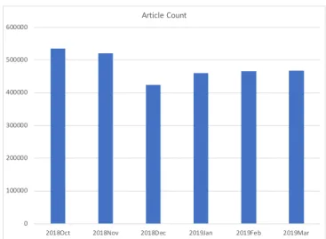
The 6-month data set includes news articles from October 2018 to March 2019. No selections were made to this data set. The average monthly article count is about 480 thousand. Figure 3.1 shows the article counts of each month.
0 100000 200000 300000 400000 500000 600000
2018Oct 2018Nov 2018Dec 2019Jan 2019Feb 2019Mar
Article Count
Figure 3.1: Article Count of Each Month (6-month data set)
3.2.1 N gram
To represent phrases or named entities such as ‘white house’ in the word embeddings, the entities field of each news article is used. The max length of phrases is set as 4 to avoid meaningless phrases. For example, “chief investment officer of Bank of America Global Wealth and Investment Management” is a 12-word phrase found in the entities field of one article. This phrase is verbose and it is meaningless to encode this into word embeddings because this phrase may only has a frequency of 1 among all time periods. The algorithm is simple and it will turn any phrase that is less than 5 words into one word, like treating ‘white house’ as ‘white house’.
Algorithm 1N gram
1: entitylen←length ofentity 2: if entitylen<5then
3: joined←each word inentity with ” ”
CHAPTER 4
Results
In this section, I visualize word embeddings in 2D spaces for two words in the 2-month data set and three words in the 6-month data set. I directly list nearest neighbors of the given key word inside a table to make the sanity check for the dynamic word embeddings of 6-month data set. In addition, I define the absolute drift as a metric to detect words that change the most relative to the given key word.
4.1
2-month Data Set
The t-SNE embedding method [MH08] is used to visualize the shifts of a word in two
di-mensions. First, given a word w that we are interested in, the nearest neighbors of w at
different time periods are put together. Next, the t-SNE embeddings of these word vectors are calculated and visualized in a 2D plot.
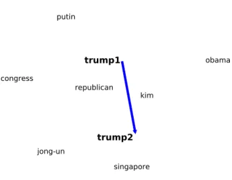
Figure 4.1 visualizes the shift of the word ‘trump’ in this 2-month data set. The word ‘trump1’ is the embedding obtained from the May 2018 word embeddings model, while
‘trump2’ is obtained from the June 2018 model. The shift of the word ‘trump’ makes
sense because the 2018 North Korea-United States Summit took place on June 12, 2018 in Singapore. As we can observe from this figure, before the summit, the word vector of ‘trump’ was close to other political terms such as ‘putin’ (the President of Russia) and ‘republican’. During the summit or afterwards, the word embedding of ‘trump’ shifts closer to ‘jong-un’ (the President of North Korea), and ‘singapore’ (the country that hosted this summit).
Figure 4.2 visualizes the shift of the word ‘Croatia’ in 2018 FIFA World Cup, which took place in Russia from 14 June to 15 July 2018. Croatia is a country at the crossroads of
trump1
trump2
congress obama republican putin kim singapore jong-unFigure 4.1: Shift of the Word ‘Trump’ (2-month data set)
Central and Southeast Europe. The Croatia national soccer team participated in this World Cup and achieved second place. The word ‘croatia1’ is the embedding obtained from the May 2018 word embeddings model (i.e. before the World Cup), while ‘croatia2’ is obtained from the June 2018 model.
Before the event started, ‘croatia’ was close to random soccer players whose teams ap-peared in 2018 World Cup as well, such as ‘firmino’ (Brazilian professional soccer player), and ‘gerrard’ (former English professional soccer player). This makes sense as word embed-dings are trained with news articles related to sports. After the FIFA World Cup began, we can observe that the word ‘croatia’ shifts closer to ‘denmark’, and ‘nizhny’. ‘Nizhny’ Novgorod Stadium is the place where ‘Croatia’ National Team defeated ‘Denmark’ National Team in the round of 16.
To clarify, the remaining two words are people related to soccer. ‘Xhaka’ is a Swiss professional soccer player, and ‘Sampaoli’ is the coach of Argentina National Soccer Team.
croatia1
croatia2
switzerland xhaka gerrard firmino denmark sampaoli nizhnyFigure 4.2: Shift of the Word ‘Croatia’ in 2018 FIFA World Cup (2-month data set)
4.2
6-month Data Set
4.2.1 2D Visualization
As stated above, the t-SNE embedding method is used to project the word embeddings
into two dimensions. First, given a word w that we are interested in, the top 10 and
non-repeating nearest neighbors ofw at different time periods are put together. Next, the t-SNE
embeddings of these word vectors are calculated and then visualized in a 2D plot.
4.2.1.1 The Word ‘Stock’
Figure 4.3 visualizes the shifts of the word ‘stock’ from October 2018 to March 2019. Different suffixes represent different months. The word ‘stock1’ is the embedding obtained from the October 2018 word embeddings model, ‘stock2’ from the November 2018 model, and so on. For the purpose of interpretation of this figure, we can roughly treat the left side of the plot as the negative sentiment towards the stock market (e.g. ‘sell-off’ and ‘selloff’) and the right side as the positive sentiment (e.g. ‘bullish’, ‘gains’, and ‘earnings’). This is further confirmed by Figure 4.4.
Figure 4.3: Shifts of the Word ‘Stock’ (6-month data set)
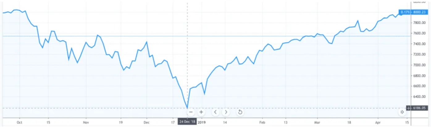
Figure 4.4 shows changes of the Nasdaq Composite Index from October 2018 to March 2019. The stock market dropped all the way down until the beginning of 2019, which confirms the closer distance between ’stock1’, ’stock2’, ’stock3’, ’stock4’ and ’sell-off’ in Figure 4.3. Then, stock market rebounded from January this year, which confirms the closer distance between ’stock5’, ’stock6’ and ’gains’ or ’earnings’ in Figure 4.3.
4.2.1.2 The Word ‘US-Mexico’
Figure 4.5 visualizes the shifts of the word ‘us-mexico’ from October 2018 to March 2019. Similar to the previous example, different suffixes represent the embeddings obtained from models of different months.
One of President Trump’s election promises was to “solve” unauthorized immigration across the southern border of United States by building a much larger and fortified border wall. Unauthorized immigrants to the southern border are not only from Mexico, but also from Central American countries such as Guatemala and Honduras, due to the increase in
Figure 4.4: Nasdaq Composite Index (6-month)
violence and abuse in recent years. To cross the Mexico-United States border, these migrants have to cross the Guatemala-Mexico border.
As a result, the immigration and border are always the top topics in news articles about US-Mexico. Figure 4.5 confirms this by showing that ‘border’, ‘us customs’, ‘crossings’ and ‘guatemalan’ are always around the word ‘us-mexico’ at different months.
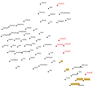
4.2.1.3 The Word ‘Max’
Figure 4.6 visualizes the shifts of the word ’max’ from October 2018 to March 2019. Different suffixes represent the embeddings obtained from models of different months.
The Boeing 737 MAX is the new generation aircraft produced by The Boeing Company. It was first delivered on May 2017, and has received thousands of orders. However, on 10 March 2019, the MAX aircraft Ethiopian Airlines Flight 302 crashed six minutes after takeoff. All 157 people aboard were killed in the accident. After this fatal crash, aviation authorities around the world grounded the Boeing 737 MAX series.
Figure 4.6 shows that word embeddings capture this sudden trend change. Before March 2019 (from when the ‘max6’ embedding is obtained), the embedding of the word ‘max’ was close to different family names or ‘xs’ (this refers to the name iphone xs max). When the Boe-ing 737 MAX crash happened or afterwards, the embeddBoe-ing of the word ‘max’ immediately shifts to words such as ‘boeing’, ‘737’, ‘aircraft’ and ‘grounding’.
Figure 4.5: Shifts of the Word ‘US-Mexico’ (6-month data set)
4.2.2 Table
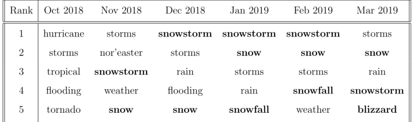
As we now have models from 6 different time slices, it may also show some interesting results if we simply list the top nearest neighbors (words that have highest cosine similarities with
the key word) of the key word w inside a table. Also, this table can function as the sanity
check for the quality of word embeddings.
Rank Oct 2018 Nov 2018 Dec 2018 Jan 2019 Feb 2019 Mar 2019
1 hurricane storms snowstorm snowstorm snowstorm storms
2 storms nor’easter storms snow snow snow
3 tropical snowstorm rain storms storms rain
4 flooding weather flooding rain snowfall snowstorm
5 tornado snow snow snowfall weather blizzard
Table 4.1: Top 5 Words closest to the Word ‘Storm’ in Each Month (6-month data set)
Figure 4.6: Shifts of the Word ‘Max’ (6-month data set)
each month. Snow is the most common thing from December to February, and the first ranked word of each month verifies this point. While in some areas of the West and Plains where extreme weather easily happens, snow is common in November or March as well. For example, Denver has an average March snowfall of 10.7 inches. This could explain why the word ‘snowstorm’, although not the first ranked word, appears in November and March.
As a point of clarification, the word “nor’easter” (rank 2 in November 2018) refers to
a macro-scale extratropical cyclone in the western North Atlantic ocean. Extratropical
cyclones are low-pressure areas along with the anticyclones of high-pressure areas, that can produce anything from mild showers to thunderstorms, blizzards, and tornadoes.
4.2.3 Find Changing Words with Absolute Drift
Inspired by [RB18], I define a metric that is more suitable to detect which words change the most relative to the key word wk. Denote cossim(wk, wi, t) as the cosine similarities between the word wi and the key word wk at timet. For top n words close to wk, calculate
the absolute drift of each word wi by summing the cosine similarity differences. drif t(wi) = T X t=2 |cossim(wk, wi, t)−cossim(wk, wi, t−1)|
In other words, the drift can help find words that fluctuate the most. After finding meaningful words that fluctuate a lot, cosine similarities between these words andwk of each month can be plotted to present possible useful interpretations.
4.2.3.1 ‘Trade-War’
18oct 18nov 18dec 19jan 19feb 19mar time 0.1 0.2 0.3 0.4 0.5 0.6 0.7 word similarity
words similarities vs. trade-war
tensions uncertainty sell-off
Figure 4.7: Cosine Similarities with ‘Trad-War’ (6-month data set)
Figure 4.7 displays the cosine similarity changes between the word ‘tensions’, ‘uncer-tainty’, ‘sell-off’ and ‘trade-war’. The blue line represents the word ‘tensions’, the orange line refers to ‘uncertainty’, and the green line is ‘sell-off’. We can infer from this figure that as the tensions and uncertainty of the trade-war grow, the stock market reflects this greater negative sentiment by the increasing sell-offs.
18oct 18nov 18dec 19jan 19feb 19mar time 0.3 0.4 0.5 0.6 0.7 word similarity
words similarities vs. unemployment
gdp boosting record-low
Figure 4.8: Cosine Similarities with ‘Unemployment’ (6-month data set)
4.2.3.2 ‘Unemployment’
Figure 4.8 displays the cosine similarity changes between the word ‘gdp’, ‘boosting’, ‘record-low’ and ‘unemployment’. The blue line represents the word ‘gdp’, the orange line refers to ‘boosting’, and green line is ‘record-low’. One thing we can infer from this figure is that as the economy (‘gdp’) shows a strong signal (‘boosting’) in the first quarter of 2019, the unemployment rate reaches a ‘record-low’ position.
According to National Public Radio, the first quarter’s gross domestic product grew at an annual rate of 3.2%, which is a strong improvement compared to the 2.2% at the end of last year. In addition, the Labor Department reported that 196,000 jobs were added in March, and the unemployment is near 50-year lows.
CHAPTER 5
Discussion
Dynamic word embeddings method is a good tool to analyze news. In this the-sis, the news articles data provided by Taboola are divided into different slices by month. Word2vec is applied to train the word embeddings models for different time periods. To con-nect word vectors from different time slices, different models are aligned through embedding space transformation.
The t-SNE method is used to visualize word embeddings in two dimensions. The 2-month data set shows pretty interesting shifts of certain words, such as Trump and Croatia. Trump becomes closer to Kim Jung Un and Singapore during the 2018 North Korea-United States Summit and Croatia becomes closer to Denmark and other teams during the FIFA World Cup. Next, more research is done on the 6-month data set. 2D visualizations on this data set reveal meaningful insights of word trend changes. For example, the shifts of the word ‘stock’ represent the sentiment change towards the stock market, which correlates with the rise and fall of the Nasdaq Composite Index over the same time periods. The shifts of the word ‘US-Mexico’ demonstrate the persisting topic of unauthorized immigrants across the US-Mexico border. The shifts of the word ‘max’ capture the instant topic trend of Boeing 737 Max crash on 10 March 2019.
Directly listing nearest neighbors of the key word inside a table presents a good way to perform the sanity check for word embeddings models. By calculating the absolute drift, some meaningful words that change the most can be found and presented in a line chart. For example, as the tensions and uncertainty of the trade-war grow, the stock market reflects this with a more negative sentiment. When the economy grows more, the unemployment reaches a record-low position.
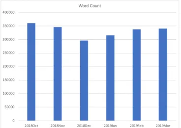
Although many interesting and meaningful analyses from dynamic word embeddings are presented, there are improvements that can be done in the future. One is collecting more news articles to increase the number of words per time-period. The 6-month data set has an average about 332 thousand words per month after filtering out the words that only have a frequency of 1, as shown in Figure 5.1. If each month has more than 100 million words, the quality of word embeddings models should be much better, as William L. Hamilton mentioned. Another direction is to define more evaluation methods to analyze the quality of word embeddings. 0 50000 100000 150000 200000 250000 300000 350000 400000
2018Oct 2018Nov 2018Dec 2019Jan 2019Feb 2019Mar
Word Count
REFERENCES
[BDV03] Yoshua Bengio, R´ejean Ducharme, Pascal Vincent, and Christian Jauvin. “A
neural probabilistic language model.” Journal of machine learning research,
3(Feb):1137–1155, 2003.
[BM17] Robert Bamler and Stephan Mandt. “Dynamic word embeddings.” InProceedings
of the 34th International Conference on Machine Learning-Volume 70, pp. 380– 389. JMLR. org, 2017.
[DDF90] Scott Deerwester, Susan T Dumais, George W Furnas, Thomas K Landauer, and
Richard Harshman. “Indexing by latent semantic analysis.” Journal of the
Amer-ican society for information science, 41(6):391–407, 1990.
[HLJ16] William L Hamilton, Jure Leskovec, and Dan Jurafsky. “Diachronic word
embed-dings reveal statistical laws of semantic change.” arXiv preprint arXiv:1605.09096, 2016.
[LB96] Kevin Lund and Curt Burgess. “Producing high-dimensional semantic spaces from
lexical co-occurrence.” Behavior research methods, instruments, & computers,
28(2):203–208, 1996.
[MCC13] Tomas Mikolov, Kai Chen, Greg Corrado, and Jeffrey Dean. “Efficient estimation
of word representations in vector space.” arXiv preprint arXiv:1301.3781, 2013.
[MH08] Laurens van der Maaten and Geoffrey Hinton. “Visualizing data using t-SNE.”
Journal of machine learning research,9(Nov):2579–2605, 2008.
[MSC13] Tomas Mikolov, Ilya Sutskever, Kai Chen, Greg S Corrado, and Jeff Dean. “Dis-tributed representations of words and phrases and their compositionality.” In Advances in neural information processing systems, pp. 3111–3119, 2013.
[MSF17] Christopher Manning, Richard Socher, Guillaume Genthial Fang, and Rohit Mundra. “CS224n: Natural Language Processing with Deep Learning1.” 2017. [PSM14] Jeffrey Pennington, Richard Socher, and Christopher Manning. “Glove: Global
vectors for word representation.” InProceedings of the 2014 conference on
empir-ical methods in natural language processing (EMNLP), pp. 1532–1543, 2014.
[RB18] Maja Rudolph and David Blei. “Dynamic embeddings for language evolution.” In
Proceedings of the 2018 World Wide Web Conference on World Wide Web, pp. 1003–1011. International World Wide Web Conferences Steering Committee, 2018.
[Sch66] Peter H Sch¨onemann. “A generalized solution of the orthogonal procrustes
prob-lem.” Psychometrika, 31(1):1–10, 1966.
[Seb02] Fabrizio Sebastiani. “Machine learning in automated text categorization.” ACM
[SPW13] Richard Socher, Alex Perelygin, Jean Wu, Jason Chuang, Christopher D Manning, Andrew Ng, and Christopher Potts. “Recursive deep models for semantic
compo-sitionality over a sentiment treebank.” In Proceedings of the 2013 conference on
empirical methods in natural language processing, pp. 1631–1642, 2013.
[YSD18] Zijun Yao, Yifan Sun, Weicong Ding, Nikhil Rao, and Hui Xiong. “Dynamic word
embeddings for evolving semantic discovery.” InProceedings of the Eleventh ACM
International Conference on Web Search and Data Mining, pp. 673–681. ACM, 2018.