HMM Mixtures (HMM2) for Robust Speech Recognition

(1)

E

S

E

A

R

C

H

R

E

P

R

O

R

T

I

D

I

A

P

D a l l e M o l l e I n s t i t u t e f o r P e r c e p t u a l A r t i f i c i a l I n t e l l i g e n c e•P. O. B o x 5 9 2•

Martigny•Valais•Switzerland

phone +41−27−721 77 11

fax +41−27−721 77 12

e-mail [email protected]

internet http://www.idiap.ch

HMM Mixtures (HMM2)

for Robust Speech Recognition

Katrin Weber

a

IDIAP RR 03-34

June 2003

PUBLISHED AS

Docteur ès Sciences thesis no. 2790 (2003),

Swiss Federal Institute of Technology Lausanne (EPFL), Lausanne, Switzerland.

a_{with the Dalle Molle Institute for Perceptual Artificial Intelligence (IDIAP), CH-1920 Martigny,}

Switzerand, and with the Swiss Federal Institute of Technology Lausanne (EPFL), CH-1015 Lau-sanne, Switzerland

(2)

(3)

To Peter for his love and his continuous support in good and bad times throughout this thesis

To Laura Lou for her smiles and the energy they gave me when I needed it most

To my parents for their perspective about the relative importance of a thesis and other things in life

(4)

(5)

Abstract

State-of-the-art automatic speech recognition (ASR) techniques are typically based on hidden Markov models (HMMs) for the modeling of temporal sequences of feature vectors extracted from the speech signal. At the level of each HMM state, Gaussian mixture models (GMMs) or artiﬁcial neural networks (ANNs) are commonly used in order to model the state emission probabilities. However, both GMMs and ANNs are rather rigid, as they are incapable of adapting to variations inherent in the speech signal, such as inter- and intra-speaker variations. Moreover, performance degradations of these systems are severe in the case of unmatched conditions such as in the presence of environmental noise. A lot of research effort is currently being devoted to overcoming these problems.

The principal objective of this thesis is to explore new approaches towards a more robust and adap-tive modeling of speech. In this context, different aspects of the modeling of speech data with HMMs and GMMs are investigated. Particular attention is given to the modeling of correlation. While correla-tion between different feature vectors (corresponding to temporal correlacorrela-tion) is typically modeled by the HMM, correlation between feature vector components (e.g., correlation in frequency) is modeled by the GMM part of the model. This thesis starts with the investigation of two potential ways to improve the modeling of correlation, consisting of (1) a shift of the modeling of temporal correlation towards GMMs, and (2) the modeling of correlation within each feature vector by a particular type of HMM. This leads to the development of a novel approach, referred to as “HMM2”, which is a major focus of this thesis.

HMM2 is a particular mixture of hidden Markov models, where state emission probabilities of the temporal (primary) HMM are modeled through (secondary) state-dependent frequency-based HMMs. Low-dimensional GMMs are used for modeling the state emission probabilities of the secondary HMM states. Therefore, HMM2 can be seen as a generalization of conventional HMMs, which they include as a particular case. HMM2 may have several advantages as compared to standard systems. While the pri-mary HMM performs time warping and time integration, the secondary HMM performs warping and integration along the frequency dimension of the speech signal. Frequency correlation is modeled through the secondary HMM topology. Due to the implicit, non-linear, state-dependent spectral warping performed by the secondary HMM, HMM2 may be viewed as a dynamic extension of the multi-band approach. Moreover, this frequency warping property may result in a better, more ﬂexible modeling and parameter sharing. After an investigation of theoretical and practical aspects of HMM2, encouraging recognition results for the case of speech degraded by additive noise are given.

Due to the spectral warping property of HMM2, this model is able to extract pertinent structural information of the speech signal, which is reﬂected in the trained model parameters. Consequently, such an HMM2 system can also be used to explicitly extract structures of a speech signal, which can then be converted into a new kind of ASR features, referred to as “HMM2 features”. In fact, frequency bands

(6)

iv

with similar characteristics are supposed to be emitted by the same secondary HMM state. The warping along the frequency dimension of speech thus results in an adaptable, data-driven frequency segmenta-tion. In fact, as it can be assumed that different secondary HMM states model spectral regions character-ized by high and low energies respectively, this segmentation may be related to formant structures. The application of HMM2 as a feature extractor is investigated, and it is shown that a system combining HMM2 features with conventional noise-robust features yields an improved speech recognition robust-ness. Moreover, a comparison of HMM2 features with formant tracks shows a comparable performance on a vowel classiﬁcation task.

The structure of this thesis is as follows. After an introduction of the state-of-the-art in automatic speech recognition, the shifting of the modeling of time and frequency correlation towards GMMs and HMMs respectively is brieﬂy investigated. Then, the HMM2 approach is introduced, and its theory is presented. This is followed by an experimental evaluation of HMM2 on a speech recognition task. The application of HMM2 as feature extractor is investigated, and HMM2 features are compared to for-mants. Finally, the most important results are summarized, and possible future research directions are outlined.

(7)

Version abrégée

Les systèmes de l’état de l’art de reconnaissance automatique de la parole sont typiquement basés sur des modèles de Markov cachés (Hidden Markov Models, HMMs) qui modélisent des séquences tempo-relles de vecteurs acoustiques extraits du signal de parole. Au niveau de chaque état du HMM, des mix-tures de Gaussiennes (Gaussian Mixture Models, GMMs) ou des réseaux de neurones artificiels (Artificial Neural Networks, ANN) sont le plus souvent employés pour la modélisation des probabilités d’émissions. Cependant, les GMM et les ANN sont assez rigides, n’étant pas capables de s’adapter aux variations inhérentes du signal de parole, telles que les variations inter- et intra-locuteur. Beaucoup d’effort de recherche est actuellement mis en oeuvre afin de proposer des solutions à ces problèmes.

L’objectif principal de cette thèse est d'explorer de nouvelles approches vers une modélisation plus robuste et adaptative du signal de parole. Dans ce contexte, des aspects différents de la modélisation des données représentant la parole par des HMMs et des GMMs sont étudiés. Alors que la corrélation entre les différents vecteurs acoustiques (correspondant à la corrélation temporelle) est typiquement modélisée par le HMM, la corrélation entre les coefﬁcients des vecteurs acoustiques (par exemple, la corrélation en fréquence) est modélisée par le GMM. Cette thèse commence avec une étude de deux possibilités pour améliorer la modélisation de la corrélation : (1) un décalage de la modélisation de la corrélation temporelle vers les GMMs, et (2) la modélisation de la corrélation entre les composants de chaque vecteur acoustique avec un type particulier de HMM. Cela mène au développement d’une nou-velle approche, appelée “HMM2”, qui constitue un des focus principaux de cette thèse.

Un HMM2 est une mixture particulière de modèles de Markov cachés, où les probabilités d’émis-sion de chaque état du HMM temporel (dit primaire) sont modélisées avec des HMMs (dit secondaires), travaillant dans le domaine des fréquences, et qui dépendent de l’état du HMM primaire. Des GMMs de basse dimension sont utilisés pour la modélisation des probabilités d’émission de chaque état du HMM secondaire. Par conséquent, l'approche HMM2 peut être vue comme une généralisation des HMMs con-ventionnels, qui constituent en fait un cas particulier des HMM2. Un HMM2 peut avoir de nombreux avantages par rapport aux systèmes standards. Tandis que le HMM primaire effectue un “warping” (c.a.d. un regroupement) et une intégration dans la dimension temporelle, le HMM secondaire effectue un warping et une intégration dans la dimension fréquentielle du signal de parole. La corrélation en fréquence est modélisée par la topologie du HMM secondaire. En raison du warping implicite et non-linéaire effectué par le HMM secondaire, un HMM2 peut être vu comme une extension de l’approche multi-bande. En outre, le warping en fréquence peut résulter en une meilleure modélisation, plus ﬂexi-ble, permettant en plus un partage efﬁcace des paramètres. Après une étude des aspects théoriques et pratiques de l’approche HMM2, des résultats encourageants pour le cas de la reconnaissance de la parole bruitée additivement sont donnés.

(8)

vi

Grace au warping du spectre effectué par le HMM2, ce modèle peut extraire des informations perti-nentes sur la structure du signal de parole, ce qui est reflété dans les paramètres d’un modèle entraîné. Par conséquent, un tel HMM2 peut être employé afin d’extraire explicitement des structures d'un signal de parole. Ces structures peuvent être converties dans un nouveau type de coefficients, dit “features HMM2”. En fait, des bandes de fréquences montrant une caractéristique similaire sont supposées être émises par le même état du HMM secondaire. Le warping dans la dimension des fréquences génère donc une segmentation adaptable en fonction des données. Comme on peut supposer que les états dif-férents du HMM secondaire modélisent des régions de basses ou hautes énergies respectivement, cette segmentation peut être en relation avec les formants. L’applications du HMM2 comme extracteur de coefficients est étudié, et il est montré qu'un système qui combine ces “features HMM2” avec des coef-ficients conventionnels et robustes aux bruits obtient une amélioration de la robustesse en reconnais-sance de la parole. De plus, une comparaison des “features HMM2” avec les traces de formants montre des résultats comparables pour la tache de la classification de différentes voyelles.

La thèse est structurée ainsi : Après une introduction de l’état de l’art en reconnaissance automatique de la parole, le décalage de la modélisation de la corrélation temporelle et fréquentielle vers les GMMs et vers les HMMs respectivement est étudié. Ensuite, l’approche HMM2 est introduite, en commençant par la théorie. Ceci est suivi par une évaluation des HMM2 pour la reconnaissance de la parole. L’appli-cation des HMM2 comme extracteur de coefﬁcients est étudiée, et les “features HMM2” sont comparés aux formants. Finalement, les résultats les plus importants sont récapitulés, et des directions possibles pour la recherche future sont données.

(9)

Kurzfassung

Algorithmen zur automatischen Spracherkennung, die dem aktuellen Stand der Technik entsprechen, basieren in der Regel auf Hidden-Markov-Modellen (Hidden Markov Models, HMMs), die die zeitliche Abfolge von Merkmalsvektoren beschreiben. Die Emissions-Wahrscheinlichkeiten werden für jeden einzelnen Zustand des Modells meist als Mischung von Gaußkurven (Gaussian Mixture Models, GMMs) oder als künstliche neuronale Netze (Artificial Neural Networks, ANNs) modelliert. Jedoch sind sowohl GMMs als auch ANNs relativ unflexibel und können sich nicht an die für Sprachsignale typischen Variationen (z.B. zwischen verschiedenen Sprechern oder zwischen verschiedenen Aussprachevarianten desselben Sprechers) anpassen. Zudem versagen sie häufig unter gegenüber dem Trainingsfall veränderten Bedingungen, z.B. bei Hintergrundgeräuschen. Zur Zeit wird intensiv an Lösungen zu diesen Problemen geforscht.

Das hauptsächliche Anliegen dieser Arbeit ist es, neue Ansätze für eine robustere und adaptive Sprachmodellierung zu erforschen. In diesem Zusammenhang werden verschiedene Aspekte der Mo-dellierung des Sprachsignals mittels HMMs und GMMs untersucht. Besondere Aufmerksamkeit wird der Modellierung von Korrelationen geschenkt. Während die Korrelation zwischen verschiedenen Merkmalsvektoren (zeitliche Korrelation) typischerweise mit einem HMM beschrieben wird, so ist das GMM für die Modellierung der Korrelation zwischen den einzelnen Komponenten eines Merkmalsvek-tors (Korrelation bezüglich der Frequenz) verantwortlich. Diese Arbeit beginnt mit einer Untersuchung von zwei möglichen Wegen, die Modellierung der Korrelation zu verbessern. Zum einen wird eine Ver-schiebung der Modellierung zeitlicher Korrelation in Richtung eines GMM untersucht. Zum anderen wird die Modellierung der Korrelation zwischen den Komponenten eines Merkmalsvektors mit einem speziellen HMM erforscht. Dies führt zur Entwicklung eines neuen Ansatzes, der als "HMM2" bezeich-net wird und der den Fokus dieser Arbeit bildet.

HMM2 ist eine besondere Mischung aus HMMs, bei der die Emissions-Wahrscheinlichkeiten des zeitlichen (primären) HMM durch zustandsabhängige, frequenzbasierte (sekundäre) HMMs beschrie-ben werden. GMMs niedriger Dimension werden für die Modellierung der Emissions-Wahrscheinlich-keiten der Zustände des sekundären HMM genutzt. Deshalb können konventionelle HMMs als Spezialfall von HMM2 betrachtet werden. Verglichen mit Standard-HMMs hat HMM2 verschiedene potentielle Vorteile. Während das primäre HMM ein Warping (d.h. ein Verziehen) und eine Integration über die zeitliche Dimension ausführt, vollzieht das sekundäre HMM ein Warping und eine Integration über die Frequenzen des Sprachsignals. Korrelationen über der Frequenz werden durch die Topologie des sekundären HMM beschrieben. Wegen des impliziten, nicht-linearen, zustands-abhängigen spek-tralen Warpings des sekundären HMM kann HMM2 als eine dynamische Erweiterung des "Multi-Band-Ansatzes" betrachtet werden. Außerdem kann dieses Frequenz-Warping zu einer besseren, ﬂexibleren Modellierung und zu einer gemeinsamen Parameter-Nutzung führen. Nach einer Untersuchung von

(10)

the-viii

oretischen und praktischen Aspekten von HMM2 werden Erfolg versprechende Resultate für die Erken-nung von additiv verrauschter Sprache präsentiert.

Als eine Folge des spektralen Warpings extrahiert HMM2 automatisch relevante strukturelle Infor-mationen der Sprache, welche in den trainierten Parametern widergespiegelt werden. Demzufolge kann HMM2 auch zur Extraktion expliziter Strukturen aus einem gegebenen Sprachsignal eingesetzt werden. Diese können dann in eine neue Art von Merkmalsvektoren umgewandelt werden, welche "HMM2-Merkmalsvektoren" genannt werden. Tatsächlich ist anzunehmen, dass Frequenz-Bänder mit ähnlicher Charakteristik vom gleichen Zustand des sekundären HMM emittiert werden. Deswegen führt das Fre-quenz-Warping zu einer anpassungsfähigen, datengesteuerten Segmentierung des Sprachsignals entlang der Frequenz-Axe. Da angenommen werden kann, dass Regionen hoher bzw. niedriger spektraler Ener-gie durch unterschiedliche Zustände des sekundären HMM beschrieben werden, könnte sich diese Seg-mentierung an den Formanten des Sprachsignals orientieren. Die Anwendung von HMM2 zur Extraktion von HMM2-Merkmalsvektoren wird untersucht und es wird gezeigt, dass die Kombination von konventionellen (gegenüber Rauschen robusten) Merkmalsvektoren und von HMM2-Merkmals-vektoren zu einer verbesserten Robustheit der Spracherkennung führt. Außerdem zeigt ein Vergleich zwischen HMM2-Merkmalsvektoren und Formantverläufen eine vergleichbare Leistung bei der Klassi-ﬁkation von Vokalen.

Diese Arbeit ist wie folgt strukturiert: Nach einer Einführung in die automatische Spracherkennung wird die angesprochene Verschiebung der Modellierung von Zeit- und Frequenz-Korrelation in Rich-tung GMM und HMM untersucht. Anschießend wird der HMM2-Ansatz und die ihm zugrunde liegende Theorie präsentiert. Es folgt eine experimentelle Bewertung des Ansatzes mittels einer Spracherken-nungs-Aufgabe. Die Anwendung von HMM2 zur Gewinnung von HMM2-Merkmalsvektoren wird untersucht und die so extrahierten HMM2-Merkmalsvektoren werden mit den Formanten eines Sprach-signals verglichen. Abschließend werden die wichtigsten Resultate der Arbeit zusammengefasst und es werden mögliche Richtungen für die zukünftige Forschung aufgezeigt.

(11)

Acknowledgements

This thesis was hosted by IDIAP, Martigny, and carried out at EPFL, Lausanne, Switzerland. I feel very privileged for having been given the opportunity to work and study in such an extraordinary environ-ment, in different respects. I would like to express my deepest thanks to all those who directly or indi-rectly helped making this thesis possible, who provided all the means for this thesis ranging from scientiﬁc advice to moral support, and, last but not least, the necessary ﬁnancing. This thesis has been supported by the Swiss National Science Foundation with grants Nr. FN 2100-50742.97/1 and Nr. FN 2000-059169.99/1, by the NCCR (IM)2 project on Interactive Multimodal Information Management, and by additional funding from IDIAP.

I would like to thank Prof. Hervé Bourlard for directing this thesis throughout the years, in spite of the fact that it was not always easy. I also profited from the scientific advice of different advisors, and from discussion with many of my colleagues, for which I am most grateful. In particular, I would like to thank Dr. Chafic Mokbel and Dr. Souheil Ben-Yacoub for having supported my early work. I am also especially indebted to Dr. Samy Bengio, whose competence, sincerity, and integrity greatly contributed to the quality of work and scientific exchange. His advice was always highly appreciated. Special thanks go to Febe de Wet and her colleagues from the University of Nijmegen for our fruitful collaboration. This document also profited from valuable comments, corrections, and other help from my colleagues and friends, particularly from Dr. Iain McCowan, Darren Moore, Jo Moore, Shajith Ikbal, Dr. Sebastian Möller, and Gianni Pante. I would also like to thank the president and the members of my thesis com-mittee for having accepted to judge this work. Many thanks to the IDIAP system group for their support with hard- and software, and to the IDIAP administration and secretariat for their help with organiza-tional problems.

The years I spent working on my thesis coincided with a particularly turbulent time in my life. It was a time of interesting professional, but also of profound personal experiences. The time of my thesis was a period of intensive and constant learning, both about speech recognition research and about some more general aspects of the functioning of the world. I appreciate all the lessons I had the chance to learn. I would like to express my gratitude to my family and friends who helped me navigate through these ups and downs. More particularly, I would like to thank those who provided some practical help at difﬁcult times, but also those who simply shared some good moments with me over the years, moun-taineering, hiking, mountain biking, snowboarding, dancing, international cooking, etc. All this helped me to get my mind off work, and, full of new energy, back on track again.

However, those who gave the most in order for this thesis to come to an end are my husband Peter and our daughter Laura Lou. While Laura Lou had to put up with her mummy going to work from a very tender age, and with long and not always easy days in the nursery, Peter greatly compensated for this with his presence, whenever possible. In a difﬁcult personal situation, he encouraged me very much in the decision to pursue my work, knowing that this meant an extraordinary additional load for him also. In addition to him being such a marvellous father and husband, he gave me a lot of practical as well as emotional support. This thesis would simply not have been possible without him.

(12)

(13)

List of Figures

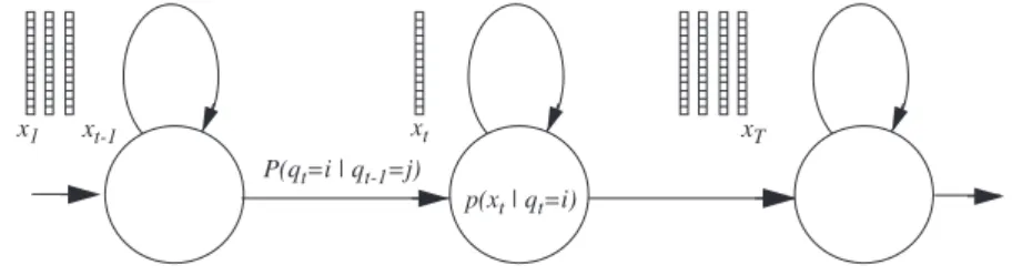
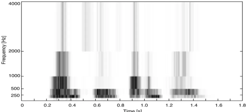
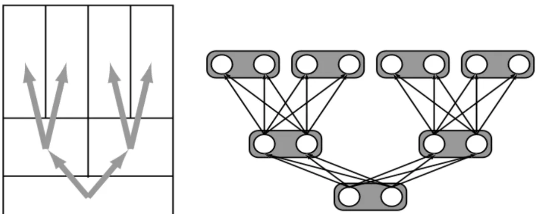
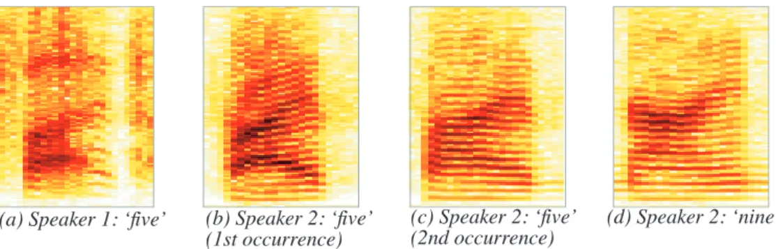
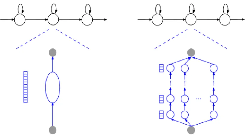
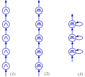
1.1 Important modules of an automatic speech recognition system. . . . . 1.2 Left-right Hidden Markov Model (HMM).. . . . 2.1 Aurora database: Percentage of relative WER ratio of the multiple time scale systems (from Tables 2.1 and 2.2) as compared to the baseline. Positive values mean a decrease in WER, i.e., a better recognition performance.. . . . 2.2 Wavelet features obtained from the Numbers95 database: The words pronounced are “one two seven three”. Dark/light regions correspond to high/low energy coefficients. . . . . 2.3 WHMT concept. The left panel shows a schema of the time-frequency plane of the lowest three resolution levels of a wavelet feature vector. The dependencies between coefficients, which are directly considered in the WHMT, are visualized by arrows. In the right panel, the corresponding WHMT is shown. Each wavelet coefficient corresponds to one node (grey in the figure), which in turn consists of two states (white circles). Transitions are introduced be-tween the states of adjacent resolution levels, as shown in the figure. . . . 2.4 Combination of WHMTs and GMMs (taking as features wavelet coefficients and MFCCs re-spectively), and integration into temporal HMM system.. . . . 3.1 Spectrograms of different pronunciations of the phoneme /ay/ by different speakers and in different contexts. Dark regions correspond to high, light regions to low energy spectral com-ponents. The vertical axis is the frequency, the horizontal one the time evolution. . . . 3.2 HMM2 system. In the upper part, a conventional HMM, working along the temporal axis, can be seen. The local emission probability calculation is done with a secondary HMM, working along the frequency axis (depicted in the lower part of the figure). . . . 3.3 Different ways to realize a GMM within the HMM2 framework. The left panel shows the triv-ial solution, where the secondary HMM consists just of one state, emitting the entire temporal feature vector at once. In the right panel, each vertical branch of the secondary HMM corre-sponds to one Gaussian mixture component. . . . . 3.4 Different secondary HMM topologies. . . . 3.5 Toy example: modeling power of GMM vs. HMM. In (a), a mixture of 3 2-dimensional Gaus-sians is defined (i.e., Gaussian means, variances and mixture weights). This GMM is visual-ized in (b). In (c), a distribution resulting from an HMM (also employing the parameters defined in (a)) is shown. . . . .

2 7 20 21 23 24 27 28 29 42 43

(18)

xvi

3.6 Toy example: demonstration of the modeling capacity of a GMM (left part of the figure) and a secondary HMM (right part) for the case of 3-dimensional data. The GMM consists of a mixture of 2 Gaussians with diagonal covariance matrices. The secondary HMM has 2 states as shown in (d), thus there are 2 possible paths through the model (see (e), which compares to (a) for the GMM case). In (f), the Gaussian components contributing to the resulting dis-tribution are depicted (compare to (b) for GMM). It can be seen that, for the case of the sec-ondary HMM, only one dimension is expanded, resulting in the distribution depicted in (g). The principal axes of this distribution are constrained to follow the axes of the coordinate sys-tem, which is not the case for the distribution resulting from the GMM (depicted in (c)). . . . 3.7 The frequency index: In (a), data assumed to be typical of the classes α and β are visualized by a black and a gray curve respectively. On the right, feature vectors (corresponding to the class α curve) as used in the secondary HMM composed of coefficients cs, their delta ds and acceleration coefficients as, as well as the frequency coefficient fs, are shown. In (b), an ex-ample frequency segmentation is shown for each class. (c) shows a structure of an HMM with alternating H and L states, which is able to model both classes. With an additional trained fre-quency coefficient (as shown in (d)), discriminability can be ensured. . . . . 4.1 HMM2 implementation with synchronization constraints and synchronization sub-vectors. The HMM2 system is emitting a sequence of (low-dimensional) components, intermitted by synchronization components at regular intervals. . . . 4.2 Correlation coefficients of FF2 features. Dark colors correspond to high correlation coeffi-cients.. . . . 4.3 Illustration of the modeling power of GMM and Markov model using real FF2 speech data. Figure (a) shows a part of a trained GMM, (b) the equivalent trained Markov model (only two dimensions are displayed). In either case, there are mixtures of 3 Gaussians. While in (a) data correlation becomes obvious, it cannot be seen in (b). . . . 4.4 Energy spectrum of a pronunciation of phoneme /ay/. Each line in the figure corresponds to one time step, and thus to one feature vector (the thick black line is the mean). . . . 4.5 Trained HMM2 parameters for different phonemes. In each column, the means of the fre-quency indices of the 4 secondary HMM states belonging to the same temporal state are vi-sualized. Vertical bars show the respective variances. The 3 columns belonging to a phoneme correspond to the 3 temporal states. It should be noted that these structures are not meant to be sufficient for phoneme discrimination.. . . . 4.6 HMM vs. HMM2 performance for frequency filtered filterbank features, illustrated by the broken and solid lines respectively, for car noise at different signal-to-noise ratios (SNR). Er-rorbars for HMM WER show the 95% confidence interval.. . . . 5.1 Illustration of time and frequency segmentations of a speech signal, as could be produced by HMM2 Viterbi decoding for the example of a 3-state temporal HMM with 4 frequency HMM states each.. . . . 5.2 Mapping of frequency segmentations to the frequency scale. . . . . 5.3 HMM2 system in its application as feature extractor. The HMM2 system is used in a first rec-ognition pass (upper part of the figure). From the temporal and frequency segmentations

de-45 46 50 52 52 52 53 54 58 62

(19)

xvii

livered as a by-product from the Viterbi algorithm, HMM2 features can be calculated and used in a conventional HMM in a second recognition pass (lower part of the figure). . . . . 5.4 Word error rates obtained using different features extracted from a MU and an HL HMM2 system (displayed by the left (blue) and right (red) bar of each cluster respectively). With each cluster of the bar graph in the upper part of the figure, one column of the table below is asso-ciated. The features that were used for the respective tests are marked with an “x”. The nota-tion “xda” signifies that addinota-tional first and second order time derivatives were used. The last row of the table shows the resulting feature dimension for each setting. . . . 5.5 Segmentations obtained (on unseen data) from (a) a single secondary HMM and (b) a full HMM2 system. In both figures, the same speech segment is shown in a spectrogram-like manner, and the overlaid horizontal lines correspond to the frequency segmentation. In (b), additional vertical lines show the temporal segmentation obtained from the full HMM2 sys-tem, where phoneme boundaries are displayed as thick lines, and transitions between tempo-ral states of the same phonemes as thin ones. . . . 6.1 Features and segmentations for an example of phoneme /iy/. Sub-figure (a) shows a spectro-gram-like representation of log Rasta PLP features, and (b) their respective first order fre-quency derivatives. In (c), the topology of the frefre-quency HMM is shown, and in (d), the frequency segmentation obtained from a forced alignments of the data in (b) given this HMM is shown in the time/frequency plane. In (e), the projection of this segmentation onto the orig-inal features is visualized. . . . 6.2 Example spectrogram and formant tracks (F1,F2 and F3) of two pronunciations of the pho-neme /er/ (pronounced within the word “heard”), as provided with the AEV database. Only the frequency band from 0-4000Hz is shown. The vertical black lines show the part which was labeled as the vowel part, according to the segmentation provided with the database. It can be seen that the formant tracks corresponding to the leading /h/ and trailing /d/ are very irregular. In the lower figure, a merger of F2 and F3 occurred, and the upper frequency slot was thus set to zero.. . . . 6.3 Frequency mapping of second-order frequency filtered filterbank features (FF2) as used in HMM2. . . . . 6.4 Features displayed in spectrogram format. Time evolution is displayed on the horizontal and frequency resolution on the vertical axis. Each square corresponds to a coefficient, where the color intensity indicates different values. In the left panel, 14 mel-scaled filterbank coeffi-cients are shown, which were used as basis in order to extract 12 FF2 features, as displayed on the right. Hand-labeled formant tracks are projected onto both sub-figures.. . . . 6.5 Hand-labeled formant tracks (left panel) and “Robust Formants” (right panel) for one exam-ple of phoneme /er/, overlaid onto a spectrogram-like representation of FF2 features. . . . 6.6 Comparison of hand-labeled formant tracks (left column) and HMM2 feature tracks (right column), overlaid onto a spectrogram of FF2 features. In (a), (b), and (c), examples of pho-neme /er/ are shown, (d) figures an example of /oa/ and (e) of /ae/. The HMM2 feature tracks of (a) and (b) were obtained using gender-dependent models, those of (c), (d), and (e) using gender-independent models. (b) and (c) are showing the same example for a direct

compari-64 66 67 75 77 81 82 85

(20)

xviii

son between HMM2 feature tracks obtained from gender-dependent and gender-independent models. . . . . 6.7 Summary of important results. The left cluster shows average classification rates for the gen-der-independent tests, the right cluster for the gender-dependent ones. The bars in each clus-ter correspond to the following features (from left to right): MFCC-13, MFCC-3, HLF, RF, and HMM2 features. Moreover, where appropriate, results using the same features with ad-ditional first order temporal derivatives are indicated with broken lines. The errorbars shown for each cluster are based on the HLF results and indicate the 95% confidence interval. . . . .

90

(21)

List of Tables

2.1 Word error rate on the Aurora database: Two time scales, the second time scale being the av-erage over 9 subsequent frames of the first time scale and consisting of 13 coefficients. . . . . 2.2 Word error rate on the Aurora database: Two time scales, the second time scale being the av-erage over about 2s of the energy coefficients of the first time scale. . . . . 2.3 Word error rate on Numbers95 for Wavelets-WHMTs, MFCC-Gaussians, and their combi-nation. . . . . 4.1 Comparison of systems using different models for the local likelihood estimation of the pri-mary HMM: WER on Numbers95. Where applicable, the numbers in superscripts designate the corresponding topology (see Section 3.3). . . . . 5.1 Word error rates using MFCC-SS, HMM2 features and their combination for clean speech and speech degraded by additive factory noise at different SNRs. . . . 6.1 Classification rates of MFCC features when used in conventional HMMs. . . . 6.2 Classification rates of FF2 features when used in conventional HMMs. . . . 6.3 Classification rates of hand-labeled formants. . . . . 6.4 Classification rates of Robust Formants.. . . . 6.5 Classification rates of HMM2 features (second pass) obtained with FA/VR. . . . . 6.6 Classification rates of FF2 features when used in an HMM2 system in the first pass (using different initializations). . . . . 6.7 Classification rates using “ideal” HMM2 features (obtained from FA/FA) in the second rec-ognition pass.. . . . A.1 Comparison of HMM2 decoder performance: WER on clean speech.. . . . A.2 Comparison of HMM2 decoder performance: WER on factory noise. . . . . A.3 Comparison of HMM2 decoder performance: WER on lynx noise.. . . . A.4 Comparison of HMM2 decoder performance: WER on car noise.. . . . B.1 Comparison of HMM2 feature performance: WER on clean speech. . . . . B.2 Comparison of HMM2 feature performance: WER on factory noise. . . . . B.3 Comparison of HMM2 feature performance: WER on lynx noise. . . . . B.4 Comparison of HMM2 feature performance: WER on car noise. . . . . C.1 Comparison (classification rates) of OM and PDM systems. . . . .

19 19 25 53 68 79 80 84 86 87 88 88 99 100 100 100 101 102 102 102 104

(22)

xx

C.2 Comparison (classification rates) of using the frequency coefficient in feature combination (FC) vs. likelihood combination (LC). For the case of LC, different stream weights have been tested and only the best results are reported here.. . . . C.3 Comparison (classification rates) of different initialization methods. . . . C.4 Comparison (classification rates) of different options for training/testing. . . .

104 104 104

(23)

Chapter 1 Introduction

One of the most fundamental characteristics distinguishing humans from all other living beings is the use of high level spoken language for communication. The importance of the use of speech is already reflected in old science fiction movies, where computers understood humans. For example, already in the 1960s, the makers of “2001: A Space Odyssey” depicted a sophisticated system that allowed humans to talk to computers. Also researchers were realizing that using spoken language is indeed one of the most natural and efficient ways for humans to communicate and that it could be very valuable to use such a communication scheme with computers as well. Today, as the scientific progress (as well as the industrial and economic environment) allow advanced technology for computer access, this concept is penetrating many fields of our daily lives. However, the use of spoken language for human-computer interaction is still restricted to specific, limited domains. For instance, current automatic speech recogni-tion (ASR) systems typically only deal either with a limited vocabulary (such as in voice dialing appli-cations which come with many commercial cellular phones), or they need to be adapted to a certain speaker (such as in dictation systems). Moreover, these ASR systems almost inevitably fail in spontane-ous speech and in other difficult conditions such as under environmental noise, where human speech recognition hardly degrades.

A lot of research effort is currently spent in laboratories all around the world in order to alleviate these problems, and several approaches towards this goal are also investigated in our institution. The goal of improving ASR robustness defines also the framework of this thesis. More particularly, on the base of state-of-the-art speech recognition technology, new approaches towards a more robust and adap-tive modeling of speech are investigated. To first give an introduction of the state-of-the-art in automatic speech recognition (ASR), this chapter starts with an illustration of the structure of a typical ASR sys-tem and a discussion of its major modules. Then, weaknesses of this standard syssys-tem are reviewed, and some approaches towards alleviating them are discussed. Finally, this thesis is placed into the defined context, and its history and outline are given.

1.1 Automatic Speech Recognition

Figure 1.1 shows a block diagram of an automatic speech recognition (ASR) system. It shows three major modules: (1) feature extractor, (2) acoustic model, and (3) decoder. The feature extractor provides salient feature vectors at regular time intervals. The resulting features are aimed at characterizing the linguistic information of the speech signal and discarding all other sources of variability. They are then used in the acoustic model, which typically produces a measure of similarity between each temporal

(24)

2 Introduction

feature vector and the relevant speech units (classes). This measure most often corresponds to the prob-ability (or likelihood) of a temporal feature vector belonging to a certain class. Finally, the (global) decoder is responsible for the temporal alignment and integration of these (local) similarity measures, thereby also taking account of lexical, grammatical and possibly even semantic constraints deﬁned by the language model.

However, it needs to be clariﬁed that the representation of ASR in those few distinct modules is rather arbitrary and adapted to the point of view on ASR we adopt in the framework of this thesis. Dif-ferent representations of ASR system architectures may be found e.g. in Gold and Morgan (2000), Huang, Acero, and Hon (2001) and Bilmes (1999a). For example, before feature extraction, one might want to add distinct modules for signal acquisition and analog-digital conversion. In spite of their importance for the quality of an ASR system, these issues are out of the scope of this thesis and are therefore not discussed here. Consequently, as the starting point of our ASR system, we take the digi-tized waveform for granted. Similarly, we are here not concerned with higher level language modeling (which includes dictionary, grammar, and possibly even semantics). However, the language model is implicitly considered during decoding and therefore displayed in the ﬁgure.

The figure might also suggest that the modules are distinct and well-defined, and that e.g. a certain feature extractor could be replaced by another while leaving the rest of the ASR system unchanged. However, this is not necessarily the case, as the subsequent modules might be adapted to the output of the feature extractor - or the other way around, e.g. when features are searched for which satisfy certain constraints (assumptions) imposed by the subsequent modules. In fact, an ideal feature extractor could render other system modules superfluous (or at least much simpler). While this is far from reality, it is true that there is some overlap between the different modules. As an example, speech recognition improvements in the case of environmental noise might be achieved at the level of the acoustic features and/or through adaptation of the acoustic model.

In the following, we will give a short introduction to what could be called a standard speech recogni-tion system. By this we mean readily available and widely employed techniques which fit quite nicely in the three basic ASR system modules shown in Figure 1.1. There is a wide variety of feature extraction techniques, of which the ones which are most commonly used as well as those directly relevant to this thesis are discussed in Section 1.2. Most of today’s ASR systems use either Gaussian Mixture Models (GMM) or Artificial Neural Networks (ANN) for the acoustic modeling, the former of which will be used throughout this work and is therefore briefly explained in Section 1.3. Finally, virtually all ASR systems are based on Hidden Markov Models, as introduced in Section 1.4, for the temporal decoding part. decoder feature extractor language model recognized word sequence p(x|q) acoustic model

(25)

1.2. Features for Automatic Speech Recognition 3

1.2 Features for Automatic Speech Recognition

The goal of feature extraction for ASR is to provide representation of speech which permits to distin-guish between the different sounds of a language, but which is at the same time insensitive to all non-linguistic variations such as speakers’ characteristics and environmental inﬂuences and distortions (e.g., noise). That means that these features should be relatively stable for different examples of the same speech units, even if pronounced by different speakers and in different conditions. A cepstral representa-tion of the speech signal, where knowledge about the human auditory system has been incorporated in the feature extraction process, seems to be dominant in state-of-the-art ASR systems (Gold and Morgan, 2000) and will be described in the following. Moreover, some extensions, variants and alternative speech representations will be discussed.

1.2.1 Mel-Frequency Cepstral Coefﬁcients (MFCCs)

The mel cepstrum (Davis and Mermelstein, 1980) is one of the most widely employed signal represen-tations in ASR. The exact details of how MFCCs can be calculated are covered in much of the ASR lit-erature (Gold and Morgan, 2000; Rabiner and Juang, 1993; Huang, Acero, and Hon, 2001) and need not concern us here. For us, it is sufﬁcient to know that spectral analysis is followed by an integration of the power spectrum within about 20-26 triangular, overlapping ﬁlters which are equally spaced along the Mel scale. The Mel scale is perceptually motivated. It is supposed to model the sensitivity of the human ear, which has been shown to distinguish far better between close sounds in low than in high frequencies (Huang, Acero, and Hon, 2001; Rabiner and Juang, 1993). The Mel scale can be approximated by the following equation (Young et al., 1995):

. (1.1)

The resulting filter magnitudes are then pre-emphasized (to approximate the unequal sensitivity of human hearing at different frequencies) and logarithmically compressed (to model the power law of human hearing). Finally, an orthonormal transformation (usually the Discrete Cosine Transform, DCT) is applied to calculate MFCCs. Typically, only the first 13 MFCCs are used for ASR, including the -th coefficient as a measure of the energy.

1.2.2 Temporal Derivatives

Features like MFCCs as discussed above provide a good smooth estimate of the local short-term spec-trum (Gold and Morgan, 2000). However, one of the dominant characteristics of the speech signal is its dynamics. In fact, temporal changes were shown to be important for human speech recognition (Huang, Acero, and Hon, 2001). Also for ASR, they can represent discriminant information, which might not be sufficiently captured in the so-called static cepstral coefficients described above. The conventional way to include information on these dynamics is to augment the static feature vectors with temporal deriva-tives. First and second order temporal derivatives (also called delta and acceleration coefficients, denoted by D and A respectively) can be estimated by using regression equations (Young et al., 1995). The feature vector of 13 MFCCs is thus augmented by 13 delta and 13 acceleration coefficients, result-ing in an overall feature vector dimension of 39. MFCCs are widely employed, and often serve as a ref-erence in order to measure performance improvements of newly developed features (Bilmes, 1999a; Gales and Young, 1996; Garner and Holmes, 1998; Holmes, 2000; Hunt and Lefebvre, 1989; Kermor-vant and Morris, 1999; Macho et al., 1999, McCourt, Vaseghi, and Harte, 1998; Nadeu, Hernando and Gorricho, 1995; Okawa, Bocchieri, and Potamianos, 1998; Wassner and Chollet, 1996; Welling and

Mel f( ) 2595 ₁₀ 1 f 700 ---+     log = 0

(26)

4 Introduction

Ney, 1998; just to name a few examples). The fact that there is such a multitude of publications in this area indicates that, although MFCC (most often including temporal derivatives) seem to be a kind of “reference” features, there is still room for improvements. This is especially true in unmatched condi-tions, like under different environmental noises and in applications where signiﬁcant speaker variations can be expected. In the following, we will discuss two frequently applied approaches towards alleviat-ing the effects of such variations and thus providalleviat-ing a higher robustness to adverse conditions.

1.2.3 Feature Transformations

One way to improve standard ASR features such as MFCCs is to apply an additional transformation to the original features (Hunt and Richardson, 1990; Haeb-Umbach and Ney, 1992). These transforma-tions are based on certain statistics of the training data. Generally, they seek to orthogonalize the fea-tures and reduce the feature vector dimension, while preserving or improving class separability (and ﬁnally recognition performance). Two common examples of such transformations are Principal Compo-nent Analysis (PCA) and Linear Discriminant Analysis (LDA) (Fukunaga, 1972; Bishop, 1995, Duda and Hart, 1973).

PCA, also referred to as Karhunen-Loéve transformation, basically ﬁnds the directions of maximum variance of a given feature set in an unsupervised way. This transformation can be based on the calcula-tion of the eigenvalues and eigenvectors of the global covariance matrix of all data, regardless of the class labeling. For this reason, the transformed features might well represent the signal, but not be opti-mal for discrimination.

In contrast, LDA aims directly at improving discrimination, relying on a measure of class separabil-ity to derive a transformation. Therefore, the class labeling for the training data needs to be known. Typ-ically, we want to maximize the inter-class variance while minimizing the intra-class variance. To achieve this, a linear transformation can be derived according to different criteria, such as the trace of the ratio between inter- and intra-class covariance matrices (Fukunaga, 1972). One such transformation is thus given by the eigenvectors of this covariance ratio matrix. As the above criterion should be maxi-mized, those eigenvectors whose eigenvalues are largest should be chosen for dimensionality reduction (as is also the case for the PCA described above).

1.2.4 Noise Reduction Techniques

Another way to make standard ASR features more robust is to apply noise reduction techniques such as spectral subtraction (SS) and cepstral mean normalization (CMS) (Gold and Morgan, 2000; Huang, Acero, and Hon, 2001). These methods typically try to remove an estimate of the noise from the speech signal, thus reducing a possible mismatch between training and testing conditions in the feature space. While SS is designed to cope with additive noises (e.g., car noise, ofﬁce noise), CMS handles convolu-tional distortion (e.g. microphone or telephone distortions, reverberations).

SS is based on the assumptions that the speech signal has been corrupted by (rather stationary) addi-tive noise, and that the clean signal and the addiaddi-tive noise are uncorrelated. In order to obtain the power spectrum of the clean signal, an estimate of the noise power spectrum (typically obtained during non-speech periods) is subtracted from the power spectrum of the corrupted signal.

CMS removes the (long-term) average of the cepstrum from each cepstral feature vector. This pro-cessing is based on the fact that convolutional disturbances in the time domain become additive in the cepstral domain. As this subtraction in the cepstral domain corresponds to a division in the spectral domain, this technique is also called Cepstral Mean Normalization.

(27)

1.3. Gaussian Mixture Models (GMM) 5

1.2.5 Alternative Representations

Although MFCCs are widely employed, they are by far not the only powerful speech representation in terms of ASR performance. Another example, which is very similar to MFCCs as it is based on similar processing steps, is perceptual linear prediction (PLP), and different processing steps of the two approaches may even be combined to yield other variants of features (Gold and Morgan, 2000). Like-wise, the techniques described in Sections 1.2.2 to 1.2.4 simply represent common examples amongst a multitude of possibilities, which might be combined directly or in a different, often more sophisticated form with other feature extraction approaches. As an example, RASTA-PLP (Hermansky and Morgan, 1994) is a modiﬁed version of PLP processing which is based on ﬁltering temporal trajectories of sub-band energies. It is thus related to temporal derivatives (Section 1.2.2) and can also be interpreted as a short-time version of CMS (Section 1.2.4) (Gold and Morgan, 2000).

For some applications, it might be desirable to use features in the spectral domain. This is for instance the case in “missing data” processing (Cooke et al., 2001), as well as in the HMM2 approach which will be introduced in Chapter 4. However, depending on the kind of model used in subsequent ASR modules, common spectral representations of speech are often not competitive with features in the cepstral domain. An exception to this are the recently developed Frequency Filtered Filterbank coeffi-cients (FF) (Nadeu, 1999; Nadeu, Macho and Hernando, 2001). Frequency filtering can be applied directly to Mel frequency filterbank coefficients (obtained at an intermediate stage during the extraction of MFCCs, as explained in Section 1.2.1). Frequency filtering consists of simply calculating the differ-ence between two coefficients of the same feature vector, e.g. for first order FF coeffi-cients and for second order ones (in which case they are denoted as FF2). One of the advantageous effects of this frequency filtering is a decorrelation of the coefficients, while staying in the spectral domain. In addition, FF and FF2 features yield competitive speech recognition results to MFCCs, which makes them particularly attractive features for the applications mentioned above.

An alternative spectral representation of speech is given by wavelet coefﬁcients. A possible advan-tage of these features is their property of providing information on different resolution levels in time as well as in frequency. In fact, they offer a better temporal resolution at higher frequencies and a better frequency resolution at lower frequencies. Wavelet related features have been used in different ways in ASR (e.g., Kadambe and Srinivasan, 1994; Wassner and Chollet, 1996; Long and Datta, 1996; Long and Datta, 1998; Kryze et al., 1999; Farooq and Datta, 2001), but as yet have not been shown to be compet-itive with state-of-the-art features.

While features like MFCC are derived using knowledge about human speech perception, alternative representations consider speech production related information. Of these, formants (defined as the reso-nance frequencies of the vocal tract) are a compact and highly efficient representation of the time-vary-ing characteristics of speech (Rabiner and Juang, 1993), which are supposed to be robust in noise. Formants have been shown to be useful especially for vowel classification. In ASR, they have been used in combination with other state-of-the-art features. However, one of the drawbacks of formants lies in the difficulty of reliably estimating them, and as yet they are not widely used as features in ASR sys-tems.

1.3 Gaussian Mixture Models (GMM)

There are a number of different ways to implement the acoustic model. Of these, the most widely employed are Artiﬁcial Neural Networks (ANNs) (Bourlard and Morgan, 1994, Bourlard and Bengio, 2002) and Gaussian Mixture Models (GMMs) (Rabiner and Juang, 1993). While both these methods

x f( )–x f( –1) x f( +1)–x f( –1)

(28)

6 Introduction

exhibit certain advantages and drawbacks, they show a comparable performance (provided that suitable (possibly different) features are used for either of these two approaches). GMMs can be seen as the clas-sic approach, moreover offering a suitable framework for the issues investigated in this thesis. There-fore, we will focus on the use of GMMs for (local) acoustic modeling.

In ASR, GMMs are typically used to model the distribution of the data belonging to a certain class (e.g., phoneme or sub-phone unit, represented by the HMM states). GMMs are universal approximators of densities, i.e., given a sufﬁcient number of mixture components, they can approximate any distribu-tion (Bishop, 1995; Huang, Acero, and Hon, 2001). For the case where the covariance matrices are diag-onal, as considered here, the associated probability density function is deﬁned as follows:

, (1.2)

where is the number of mixture components and are the weights associated to the respective mix-tures, is the number of (scalar) components of a feature vector (corresponding to the feature vector dimension ), and and are the means and variances of all mixture components

and all feature vector components . The mixture weights are positive and

. (1.3)

GMMs can be trained using the Expectation-Maximization (EM) algorithm (Dempster et al., 1977). As we will discuss EM training for Hidden Markov Models (where the state probability distributions are modeled by GMMs) in Section 1.4.3, EM training for GMMs will not separately be discussed here.

1.4 Hidden Markov Models

Hidden Markov models (HMMs) can be seen as a generalization of GMMs, which are suitable for sequential data. In ASR, (ﬁrst order) HMMs are typically used to represent the density of sequences of

acoustic vectors , as shown in Figure 1.2. The basic idea

under-lying HMMs is to introduce a hidden (unknown) variable describing the state of the system at time , and to factor the density of a sequence into several more simple terms: the initial state probabilities , the state transition probabilities , and the emission probabilities . As these HMM state emission probabilities are here represented by GMMs, we refer to the entire system as Gaussian Mixture Hidden Markov Model (GM-HMM).

1.4.1 Notation

Basic notations used throughout this document are deﬁned below and visualized in Figure 1.2: • is the observed vector at time step ,

• the HMM state at time , where is a path through the HMM,

• is the HMM emission probability, where the instantiation is the probabil-ity to emit in state ,

• is the initial state probability of the HMM,

p x( ) cg 1 2πσgf 2 --- e 1 2 ---– x f µgf – σgf ---     2 ⋅ f=1 F

∏

g=1 G

∑

= G c_g F xf x d µ_gf σ_gf2 g = 1…G f = 1…F c_g cg g=1 G

∑

= 1 T X = x1 T_, = {x1, , , , ,x2 … xt … xT} qt t P q( )0 P q( t qt–1) p x( t qt) xt t qt t Q p x( t qt) p x( t qt= i) xt i P q( )0

(29)

1.4. Hidden Markov Models 7

• is the HMM state transition probability, where the instantiation is the probability to go from HMM state at time to state at time , • is the number of HMM states,

• is the size of the sequence .

The likelihood of the data sequence given the model parameters at training step is then

. (1.4)

1.4.2 HMM Assumptions

In the HMMs presented in this section, we assume that the value the hidden (state) variable takes is gov-erned by a ﬁrst order Markov process. The observations (feature vectors) then depend on the resulting assignment of this variable. We can thus formulate two conditional independence assumptions, regard-ing transition and emission probabilities. Firstly, it is assumed that the state is conditionally indepen-dent of any preceding variables given the previous state :

. (1.5)

This equation is in fact a generalization of the ﬁrst order Markov assumption. Moreover, it is assumed that the transition probabilities are independent of time, i.e., they depend only on the origin and the destination . Secondly, the probability of emitting at time depends only on the state and is conditionally independent of the past states and observations:

. (1.6)

This equation is frequently referred to as the output-independence assumption.

1.4.3 EM Training

Supposing that a sequence of acoustic vectors has been generated by a hidden Markov model, the underlying sequence of HMM states is generally not known. Therefore, the data observed is said to be “incomplete” and consequently, HMM parameters can not be estimated directly. The Expectation Max-imization (EM) algorithm offers a way to circumvent this problem, using an iterative two-step proce-dure.

The goal of the EM algorithm is to maximize the likelihood of the data , given the model parameterized by . EM solves the problem of the incomplete data by introducing hidden variables such that the knowledge of these variables would simplify the learning problem. Hence, in the ﬁrst step of each iteration (referred to as E-step), the values of these hidden variables are estimated, while in the

P q( t qt–1) P q( t=i qt–1= j)

j t–1 i t

N

T x1 T, = {x1, , ,x2 … xT}

Figure 1.2: Left-right Hidden Markov Model (HMM).

x1 xt-1 xt xT p(xt | qt=i) P(qt=i | qt-1=j) X = x1 T_, θ k L X( θ) p x1 T, θ k ( ) = qt qt–1 P q( t=i qt–1 = j,q1 t, –2,x1 t, –1) = P q( t= i qt–1= j) j i xt t qt = i p x( t qt= i,q1 t, –1,x1 t, –1) = p x( t qt =i) L X( θ) X θ

(30)

8 Introduction

second step (referred to as M-step), the expectation of the log likelihood of the observations and the hid-den variables is maximized, given the previous values of the parameters. This two-step process is repeated iteratively and is proved to converge to a local optimum of the likelihood of the observation (Dempster, Laird & Rubin, 1977).

The adaptation of EM suitable for HMMs is also referred to as “Forward-Backward” or “Baum-Welch” algorithm (Baum and Petrie, 1966; Baum et al., 1971), which is brieﬂy outlined in the follow-ing1. As stated before, for the case of HMMs the hidden variables correspond to the state assignments, i.e. the sequence of states . Introducing an indicator variable such that is deﬁned to be 1 when and 0 otherwise, the joint likelihood of the observations and the hidden variable is then given by:

. (1.7)

We further deﬁne the following auxiliary function:

. (1.8)

As stated before, the E-step consists of computing the expectations of the hidden variables, given the current parameters and the data. This can be done using a recursive estimation of some intermediate “forward” and “backward” variables (which explains the name Forward-Backward algorithm). In the M-step, given the estimated values of the hidden variables and the data, new parameters (i.e., for the transition probabilities and emission distributions) maximizing are found. Thus, at the -th iteration, one computes

. (1.9)

It can be shown that maximizing also maximizes the likelihood of the data (Dempster, Laird, and Rubin, 1977).

1.4.4 Decoding

The aim of HMM decoding is to ﬁnd the sequence of HMM states which best explains the input data, while at the same time taking account of phonological, lexical and syntactical constraints in the case of ASR. Therefore, under the typical HMM assumptions (see Section 1.4.2), the recognized word sequence can be obtained by ﬁnding the path which maximizes the joint likelihood of the data and the hidden variables, given the model parameters:

. (1.10)

This is usually done with the Viterbi algorithm (Viterbi, 1967), which is based on a recursion quite sim-ilar to the calculation of the forward variable mentioned above2.

1_{A detailed description of this algorithm can be found in Section 3.2.3.}

2_{This issue will be discussed in more detail in Section 3.2.4.}

Q Z = {zi t_, } zi t_, qt = i L X Q( , ) P q( )0 p x( t qt= i) z_{i t}_, P q( t=i qt–1 = j) z_{i t}_, _⋅z_{j t}_,_–₁ j=1 N

∏

i=1 N

∏

t=1 T

∏

= A(θ θk) EQ L X Q( , θ) X θ k , log [ ] = A k θk+1 m arg ax θ A θ θ k ( ) = A L X( θ) Q* Q* arg axm Q P q( )0 _t ₁[p x( t qt)P q( t qt–1)] = T

∏

=

(31)

1.4. Hidden Markov Models 9

1.4.5 Automatic Speech Recognition using HMMs

In automatic speech recognition, HMMs are used to model the different speech units. Typically, these speech units correspond to phonemes, and each phoneme model comprises several states (often con-nected in a left-right topology with loops, as shown in Figure 1.2). Words can be considered as concate-nations of phonemes. Hence, to obtain a word model, the relevant phoneme models can be concatenated to form one large HMM (where the dictionary deﬁnes the sequence(s) of phonemes of which a word may be composed). Similarly, sentences are sequences of words, and a sentence model corresponds to a concatenation of word models. For this case, the grammar can deﬁne possible sentences, or, alterna-tively, the probability of a certain sequence of words.

It is usually not possible to train each phoneme model separately, as the phoneme boundaries are not known (and accurately segmenting a database in terms of phonemes is a hard and highly time-consum-ing task). Therefore, “embedded traintime-consum-ing” can be used, where one large HMM is created as the concate-nation of the phoneme models corresponding to the pronounced word or sentence. This typically only requires a transcription (i.e., sequence of words) and a dictionary. All phoneme models can then be trained simultaneously using the EM algorithm described in Section 1.4.3.

The aim of speech recognition is to find the sequence of pronounced words, given an acoustic sequence. This is done by searching for the sequence of words, and thus phonemes and states, which best explains the input data. For this, the Viterbi algorithm (briefly introduced in Section 1.4.4) is usu-ally applied. Obviously, the resulting sequence of states is constrained to be of the same length as the input sequence to be recognized. Further constraints are provided through dictionary and grammar (and possibly even semantics), which can be considered parts of the language model and are highly depen-dent on the application. An adapted definition of the language model can significantly reduce the search space during decoding, making speech recognition more accurate and more efficient. However, these aspects of ASR will not be further investigated in this thesis.

In the following, we will again focus our attention on HMMs, and discuss particularly their weak-nesses and limitations.

1.4.6 Weaknesses

HMMs are quite powerful statistical models which can in principal model any probability distribution over sequences. As seen above, efﬁcient training and decoding algorithms are available, so that they have become a standard in automatic speech recognition. However, it is often claimed that HMMs suffer from a number of limitations. Potential (often cited) weaknesses of standard HMMs (as discussed in this chapter) with respect to their application to ASR, include

• a poor modeling of acoustic context (in fact, each observation is assumed to be conditionally independent of the past, given the current HMM state, and therefore all the context should be reﬂected in the assignment of the (discrete) state variable),

• the assumption that speech can be well represented by a succession of steady segments (repre-sented by the states) with instantaneous transitions between them (in fact, the observations are assumed to be identically distributed, given the HMM state),

• a poor modeling of duration (in fact, duration is primarily modeled by the transition probabilities and therefore supposed to follow an exponential distribution, and, moreover, the contribution of these transition probabilities to the overall likelihood score is often negligible).

(32)

10 Introduction

However, it can be argued (Bilmes, 1999a) that these weaknesses3 are generally due to practical con-straints, rather than caused by the model itself. They are not inherent properties of HMMs, but result from the way HMMs are used. Bilmes confirmed that in general, an HMM can accurately model any real-world probability distribution, given a sufficiently large number of hidden states and a sufficiently rich class of observation distributions. However, for practical problems, this typically implies a large number of model parameters, necessitating a prohibitive amount of training data.

As a consequence of the ever-persisting problem of limited training data, we have to deal with yet another weakness:

• a constrained model topology and number of parameters (typically chosen a priori).

Naturally, this problem is aggravated if there is a lot of variability in the data. For speech, this is typ-ically the case. Sources of variability include additive noises and channel distortions, but also speech and speaker variations such as voice quality, context, stress, speaking rate and style (Junqua and Haton, 1996). Although some of these distortions and variations can effectively be removed from the data (e.g., using noise reduction techniques as mentioned in Section 1.2.4), state-of-the-art ASR systems still suf-fer from

• a limited robustness in adverse conditions.

The higher the variability of the data, the higher the amount of data and the complexity of the model that is needed for an adequate data representation. Given that the amount of available training data is limited, HMMs have to be constrained. For the case of ASR, this typically results in left-right phone (or triph-one) models with a limited number of states, using a limited number of Gaussian mixtures to estimate the observation probabilities. These restricted class of HMMs is then likely to exhibit the ﬁrst set of weaknesses listed above.

Finally, another potential weakness of standard HMMs is that

• the model is usually not trained using a discriminant criterion (i.e., minimizing the classiﬁcation error (Duda and Hart, 1973)), but instead using a maximum likelihood criterion (i.e., maximizing the likelihood of the data associated with each speech unit).

Much research has been devoted to overcome at least some of these limitations (and this thesis is yet another attempt). Some of the most important achievements are described below.

1.5 Alternative Models

In the last section, we have outlined some of the weaknesses of the application of HMMs in the frame-work of ASR (which of course may equally apply to other real-world problems). It was stated that the main reason for these limitations lies in the constraints which have to be imposed on HMMs (due to a the problem of limited training data and a high variability in the data). While illustrating this statement with some examples, we will introduce attempts to overcome some of these limitations for the case where training data is limited.

With an unlimited amount of training data (including all potential sources of variability), large HMMs could be trained which could effectively approximate the real data distribution. A more realistic way to deal with this problem is to train not only the parameters of a given model, but also learn the

3_{As well as other supposed / frequently criticized weaknesses (Bilmes, 1999a), which are however closely}