To Aggregate, Pool, or Neither: Testing the Rational Expectations Hypothesis Using Survey Data

(1)

TESTING THE RATIONAL EXPECTATIONS

HYPOTHESIS USING SURVEY DATA

by

Carl S. Bonham and Richard H. Cohen

Working Paper No. 00-3R

February 2000

(2)

Hypothesis Using Survey Data

Carl S. BONHAM

and Richard H. COHEN

It is well known that even if all forecasters are rational, estimated coeﬃ-cients in unbiasedness regressions using consensus forecasts are inconsistent because forecasters have private information. However, if all forecasters face a common realization, pooled estimators are also inconsistent. In contrast, we show that when predictions and realizations are integrated and cointe-grated, micro-homogeneity ensures that consensus and pooled estimators are consistent. Therefore, contrary to claims in the literature, in the absence of micro-homogeneity, pooling is not a solution to the aggregation problem. We reject micro-homogeneity for a number of forecasts from the Survey of Pro-fessional Forecasters. Therefore, for these variables unbiasedness can only be tested at the individual level.

KEY WORDS: Rational Expectations; Micro-homogeneity; Heterogeneity Bias; Aggregation Bias; Survey Forecasts

1. INTRODUCTION

Survey data have been used extensively in direct tests of the rational expectations hypothesis (REH). (See Holden, Peel and Thompson (1985), Lovell (1986), or Pesaran (1987) for recent surveys of the literature on testing the REH.) These data are most commonly used in “consensus” form, i.e., the cross section of survey responses is averaged to form a single time series prediction. (Some authors have used other measures of central tendency, such as the median, geometric, or harmonic mean.) Testing the REH using consensus forecasts has, however, been criticized because aggregation may introduce at least two kinds of bias. Figlewski and Wachtel (1981, 1983) showed that, since each forecaster’s information set contains some private information (known only to that forecaster), least squares coeﬃcient estimates in consensus unbiasedness regressions are inconsistent. In addition, Keane and Runkle (1990) argued that consensus parameters may lead to false acceptance of the unbiasedness hypothesis because averaged data may conceal individual deviations from rationality. Thus, rationality tests need to be conducted using disaggregated data.

(3)

Rather than estimating individual regressions, Figlewski and Wachtel (1981, 1983) and Keane and Runkle (1990) advocated pooling all observations to increase degrees of freedom. However, Zarnowitz (1985) pointed out that when the target variable is constant for all forecasters in a given time period, correlation between regressor and error results in downward bias of the pooled estimator.

It is important to note that most researchers have implicitly assumed stationary targets and predic-tions. However, many macroeconomic series are integrated. For cointegrated targets and predictions, we show that when individual unbiasedness regressions share the same coeﬃcients across forecasters, i.e., micro-homogeneity exists, both consensus and pooled parameters can be consistently estimated. Furthermore, if micro-homogeneity does not hold, false acceptance of the unbiasedness hypothesis may occur in consensus tests, even in the unlikely event that oﬀsetting individual biases allow parameters to be consistently estimated. Therefore, this paper shows that micro-homogeneity is crucial for both consensus and pooled tests of the unbiasedness hypothesis.

Section 2.1 describes the two types of bias that arise from improper use of consenus forecasts, and section 2.2 describes the heterogeneity bias that arises from improper pooling. In section 3. we test micro-homogeneity in unbiasedness regressions using ﬁve forecast series from the Survey of Professional Forecasters. We extend Zellner’s (1962a) micro-homogeneity test to the case of Generalized Method of Moments (GMM) estimation and adapt a weighting matrix suggested by Keane and Runkle (1990), which accounts for the possibility that forecast errors follow moving average processes both for indi-viduals and across survey respondents. We show that for nearly all forecast series micro-homogeneity does not hold. At least for these heterogeneous forecasts, unbiasedness should only be tested at the individual level. In section 4. we conclude and discuss implications for future work.

2. TO AGGREGATE, POOL, OR NEITHER?

“[E]xpectations, since they are informed predictions of future events, are essentially the same as the predictions of the relevant economic theory” (Muth 1961, p. 316). The rational expectations literature has generally taken this well-known quote to mean that “subjective expectations of individuals are exactly the true mathematical conditional expectations implied by the model itself” (Begg 1982, p. 30, emphasis added). Thus, the representative agent models used by economists are assumed to be both “true” representations of the data generating process (DGP) for the series in question and knowable by agents when forming their expectations. In this case, individual-rational expectations will possess certain optimal properties. For example, such expectations will be unbiased: the unconditional mean of

(4)

forecast errors will be zero. These expectations will also be eﬃcient: forecast errors will be uncorrelated with information available to individual i at time t. “In practice, the DGP may well be unknowable to our limited intellect, important variables may be unobservable, and/or the stochastic mechanism need not be constant over time” (Hendry, 1993, p. 422). As a result, forecasters will make use of both public and private information and will likely have diﬀerent opinions regarding the best model (whether statistical or otherwise) of the true DGP.

Despite the potential diﬃculty in discovering the “true” DGP of any series, the unbiasedness property of Muthian rationality is often tested in the literature. For instance, individual unbiasedness has been tested by least squares (LS) estimation of

At+h=αi+βi hPi,t+ hεi,t, t= 1, . . . , T, (1)

whereAt+his the actual value of some target series in periodt+h, andhPi,tis the subjective expectation of At+h based on individual i’s time t information set, Ωi,t. The null hypothesis of unbiasedness is H0: αi = 0, βi = 1, and unbiased forecasts will have mean zero forecast errors,hηi,t =At+h− hPi,t, which are equivalent to the residuals in (1),hεi,t.

2.1 Should Consensus Forecasts Be Used in Unbiasedness Tests?

While it is possible to test rationality using individual survey forecasts, the literature has generally used aggregate measures of expectations. Tests of the unbiasedness hypothesis are typically based on estimation of “consensus” regressions such as

At+h=αc+βc hPc,t+hεc,t, t= 1, . . . , T , (2)

where hPc,t = _N1

N

i=1hPi,t, is the consensus prediction, N is the number of respondents in a survey, and the subscriptc is used to denote the consensus prediction, parameters, and residuals.

Joseph Livingston appears to have popularized the term “consensus” as a convenient summary statis-tic to denote a cross-sectional mean of individual survey forecasts. The American Heritage Dictionary

(1992) defines consensus as: “1. An opinion or position reached by a group as a whole or by majority will: The voters’ consensus was that the measure should be adopted. 2. General agreement or accord: government by consensus.” Definition 1 is clearly inapplicable since it implies that all survey respon-dents would submit the same forecast. Definition 2 is applicable if a given cross section of forecasts is sufficiently similar.

(5)

However, in their retrospective on the Survey of Professional Forecasters, Zarnowitz and Braun (1992, pp. 45-46) conclude: “The distributions of the [forecast] error statistics show that there is much disper-sion across the forecasts . . . Forecasters differ in many respects and so do their products. The idea that a close ‘consensus’ persists, i.e., the current matched forecasts are generally all alike, is a popular fiction. The differentiation of the forecasts usually involves much more than the existence of just a few outliers.” Thus, the very use of the term consensus forecast is a misnomer. The view that individual forecasts differ widely is also prominent in the literature on forecast combination. In fact, for combinations of forecasts to dominate individual predictions, it must be true that individual survey respondents make use of private information, so that individual forecasts are heterogeneous. (See Clemen (1989) for an early survey of the combination literature.)

Nevertheless, when surveys of consumer or business expectations ﬁrst became available, researchers used cross-sectional average forecasts to avoid small sample problems caused by large numbers of non-responses in individual forecast series. Many authors also used consensus forecasts as proxies for market expectations in models such as the Fisher hypothesis.

A number of authors have questioned whether consensus forecasts should be used in unbiasedness tests, due to the possibility that averaging individual forecasts may lead to parameter estimates which are biased, or at a minimum misleading. (See Figlewski and Wachtel (1981, 1983), Urich and Wachtel (1984), Keane and Runkle (1990), Batchelor and Dua (1991), Bonham and Cohen (1992), and Ehrbeck (1992).) Keane and Runkle (1990, p. 717) pointed out two problems with the use of consensus forecasts in rationality tests.

First, doing so causes serious specification bias. If forecasters are rational, their forecasts will differ only because of differences in their information sets. The mean of many individual-rational forecasts, each conditional on a private information set, is not itself a rational forecast conditional on any particular information set (see Stephen Figlewski and Paul Wachtel 1983). This seemingly minor issue can produce severe bias.

A second problem with using consensus forecasts is that this approach can maskindividual deviations from rationality [e.g.] . . . some ﬁrms are consistently optimistic about future sales while others are consistently pessimistic. Averaging expectations, however, can cancel these biases across ﬁrms so that industry mean expectations show no bias.

Thus, the literature has recognized the general problem of testing a hypothesis about individual behavior based on an average of potentially heterogeneous individual forecasts. Keane and Runkle’s

(6)

first point refers to individual forecasts which are rational yet heterogeneous, because they are based on individual-specific information. That is, while heterogeneous forecasts may differ widely over the cross section of individuals, rationality implies that parameter estimates in the individual unbiasedness regressions (1) are identical, i.e. micro-homogeneity holds. Figlewski and Wachtel (1983) showed that such informational heterogeneity can lead to biased coefficient estimates in consensus regressions.

Keane and Runkle’s second point involves individual forecasts which are heterogeneous in the sense that some irrational forecasters systematically overpredict while others systematically underpredict. Thus, parameter estimates in (1) will diﬀer, i.e. micro-homogeneity does not hold. Keane and Runkle’s concern is that the parameters in consensus regressions may lead to false conclusions about individual behavior. The following sections treat these two problems in more detail.

Heterogeneous Rational Forecasts.

Figlewski and Wachtel (1983) showed that individuals making rational forecasts, based on public and private information, will have diﬀerent forecasts. These individual-rational forecasts would pass a test of unbiasedness based on estimation of equation (1). However, because each forecaster cannot use the private information of other individuals, Figlewski and Wachtel (1983) argued that the consensus forecast is correlated with the consensus forecast error and therefore is not rational. (See also Pesaran (1987) and Batchelor and Dua (1991).) For example, suppose that realizations are generated by the following data generating process (DGP):

At+h=Xtγ+Ztω+υt, t= 1, . . . , T , (3)

whereX_tis a 1×dvector of publicly available information variables,Z_t= [Z₁_,t, . . . ,Z_N,t] is an 1×(N·m) vector of individual-speciﬁc information set variables, andυt∼iid[0, συ2]. Here we follow Figlewski and Wachtel (1983) and assume that each individual forms rational predictions ofAt+h, in the sense that he knows the structure and parameters of the DGP in (3) yet does not know any of the other forecasters’ private information. In the next section, we relax this stringent assumption and allow for heterogenous forecasts that are based on individual models which diﬀer systematically from the true DGP. Rational predictions and forecast errors for each individual are given by

Pi,t= E[At+h|Ωi,t] =Xtγ+Zi,tωi, i= 1, . . . , N , (4) ηi,t=

N

j=1

j=i

(7)

where we have dropped the subscripthon predictions and forecast errors for ease of exposition. Figlewski and Wachtel (1983) assumed thatE[Zt] =E[Z_i,t₋_ρZj,t] =E[υtXt] =E[υtZt] = 0∀i=j, t, ρ, implying that the individual forecast errors in (5) are mean zero, serially and cross-sectionally uncorrelated, and uncorrelated with the individual predictions,Pi,t. Therefore, from estimation of equation (1),plimαˆi= αi= 0,plimβˆi=βi= 1,∀i(i.e., micro-homogeneity holds), and the residuals are equal to the rational forecast errors, that is,εi,t=ηi,t.

The consensus forecast and consensus forecast error may be written as

Pc,t= Xtγ+ 1 N N i=1Zi,tωi, (6) ηc,t= N_N−1 N i=1Zi,tωi+υt. (7)

In contrast to the individual prediction errors, the presence of private information variables in the consensus forecast error sets up a correlation with the consensus forecast. As noted in Figlewski and Wachtel (1983), this correlation would lead to biased parameter estimates in the consensus regression (2). We refer to this bias as private information bias (hereafter, PIB).

Figlewski and Wachtel (1983) implicitly assumed stationarity in their proof of PIB. Yet, many eco-nomic time series are well described by integrated processes (see Nelson and Plosser (1982)), and much of the literature has tested the unbiasedness property of nonstationary forecasts. In the case of rational forecasts of nonstationary realizations, PIB does not occur. To see this, assume that the public infor-mation vector is partitioned as X_t = [X₁_,tX₂_,t], whereX₁_,t ∼I(1) is 1×d1, X2,t ∼I(0) is 1×d2,

andd1+d2=d. In addition, assume thatE[X2,t] =µ= 0, whileZt∼I(0). Under these assumptions, At+h∼I(1), whileAt+h andXtcointegrate with cointegrating vectorγ.

Note that our ﬁrst assumption, that private information is stationary, could be relaxed. IndividualZj,t vectors (not available to individuali) could include lagged individual forecasts (which are nonstationary) so long as Z_j,tωj is stationary. For instance, writeZj,t = [Pj,t−1, Pj,t−2, ηj,t−1, ηj,t−2, . . .] andωj = [ωj1, −ωj1, ωj3, ωj4, . . . , ωjm]. Thus, the integrated private information of individual j enters the DGP and individualisforecast error as a stationary forecast revision,ωj1(Pj,t−1−Pj,t−2).

BecauseZtis mean zero, stationary and serially and cross-sectionally independent, so too are the indi-vidual and consensus forecast errors. Also, they are asymptotically uncorrelated with theI(1) individual and consensus predictions. Therefore, for rational forecasts of integrated realizations, LS estimates of

(8)

unbiasedness parameters are super-consistent, even in the presence of omitted stationary variables. That is, estimates converge to their true values at rate T as opposed to the conventional√T (Stock, 1987).

We conclude that plimαî=αi = 0, plimβî=βi = 1∀i (i.e., micro-homogeneity holds). Similarly, from estimation of the consensus regression (2), plimαˆc = αc = 0, plimβˆc = βc = 1. This contrasts with the stationary case, where aggregation of rational forecasts based on heterogeneous private infor-mation results in PIB. It follows that Keane and Runkle’s (1990) first objection to testing unbiasedness using consensus forecasts is obviated when agents form rational predictions of an integrated target. Unfortunately, this same conclusion does not hold for Keane and Runkle’s (1990) second point.

Heterogeneous Irrational Forecasts

The second problem referred to by Keane and Runkle (1990) is that aggregation may mask systematic individual differences. In fact, given the complex, potentially changing nature of any DGP, it is likely that agents will differ in their choice of both public and private information set variables and in how efficiently they process the information in these variables. As a result, some agents are likely to produce forecasts which do not satisfy the optimality conditions of the REH. To see this, assume that agents use the following prediction rule in place of the rational forecast equation (4):

Pi,t=Xtγ˜i+Zi,tωi. (8) In (8), ˜γi= ∆iγ= ∆1i 0 0 ∆2i γ1 γ2

, where ∆i is ad×ddiagonal matrix with positive, negative, or zero diagonal elements. ∆1iγ1 is the parameter vector for the d1 integrated public information

variables (X1t), and ∆2iγ2 is the parameter vector for thed2 stationary public information variables

(X2t). Therefore, (I−∆i)γ contains individual i’s parameter biases. These biases may arise from differences in effort or ability of forecasters to identify a “good” statistical approximation of the DGP, differences of opinion as to the best approximation, or because of differences in the behavior of forecasters facing unforseeable changes in the DGP.

Under this irrational prediction rule, individual forecast errors may be written as

ηi,t =Xt(I−∆i)γ+ N j=1 j=i Z_j,tωj+υt. (9)

As long as some element of ∆1i or ∆2i is diﬀerent from one, individual forecast errors are no longer mean zero, serially uncorrelated and orthogonal to individual predictions, Pi,t. In particular, if some

(9)

element of ∆1i diﬀers from unity, the forecast errors in (9) will contain an I(1) componentX1t(Id1−

∆1i)γ1, where Id1 is a d1×d1 identity matrix; in general, the residuals from equation (1), εi,t, will

also contain the I(1) componentX₁_t(Id1−βi∆1i)γ1. Thus, individual unbiasedness parameter estimates

are inconsistent since (1) is a spurious regression. On the other hand, if ∆1i = Id1, so that true

parameters are used for each of theI(1) public information variables, then the residuals from estimation of equation (1) are I(0), and parameter estimates are super-consistent. In fact, plimβˆi = 1, while plimαˆi= [E[X2t](Id2−∆2i)γ2]. Thus, the forecasts contain only an additive bias term, since they are

cointegrated with the realizations. Furthermore, unlike the case of rational forecasts based on private information sets, when individuals form biased forecasts that are systematically diﬀerent, i.e., ∆i= ∆j, micro-homogeneity will generally not hold. Finally, note that allowing for bias in the ωi parameters is unnecessary. Once we have relaxed the assumption of rationality, relaxing our assumptions regarding private information does not add to the analysis.

When individuals form irrational forecasts based on the prediction rule in equation (8), the consensus forecast is given by Pc,t=Xt∆¯γ+ 1 N N i=1Zi,tωi, (10)

where ¯∆ = _N1N_i₌₁∆i. The consensus forecast error may be written

ηc,t=Xt(I−∆) +¯ N−1

N

i=1Zi,tωi+υt. (11)

Parallel to our analysis of individual forecast errors, as long as some element of ¯∆1i or ¯∆2i is diﬀerent from unity, the consensus forecast error is no longer mean zero, serially uncorrelated, and orthogonal to the consensus forecast. When some of the elements of ¯∆1 diﬀer from one, the consensus forecast

errors in (11) and consensus residuals from estimation of (2) are integrated, and thereforeplimαˆc=αc, and plimβˆc = βc (Bonham and Cohen (1999) point out a simplistic exception to these conclusions. If parameter biases (or average parameter biases in the consensus case) are identical across all I(1) public information variables, then individual and consensus regressions cointegrate, while individual and consensus forecast errors remain I(1).)

Keane and Runkle’s example of systematic over- or under-predictions implies individual forecasts which are biased as well as heterogeneous. Unlike the heterogeneity of rational forecasts based on private information, this heterogeneity results in parameter estimates in (1) that diﬀer across individuals, i.e.

(10)

0 1000 2000 3000 4000 5000 6000 0 1000 2000 3000 4000 5000 6000 At+h Pi,t

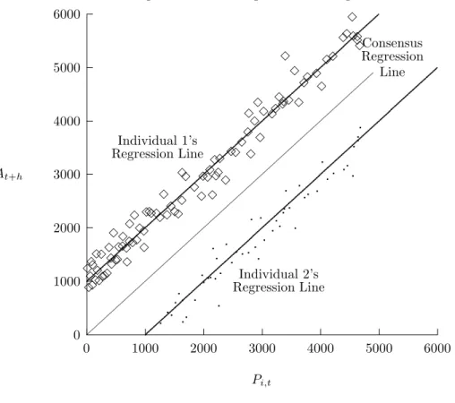
Figure 2.1 Misleading Consensus Regression

Individual 1’s Regression Line Individual 2’s Regression Line Consensus Regression Line ✸ ✸ ✸ ✸ ✸ ✸ ✸ ✸ ✸ ✸ ✸ ✸ ✸ ✸ ✸✸✸ ✸ ✸ ✸ ✸ ✸✸ ✸ ✸ ✸✸✸✸✸ ✸ ✸✸✸ ✸✸✸✸✸ ✸ ✸✸✸✸✸ ✸✸ ✸_✸✸✸✸✸_✸ ✸ ✸ ✸ ✸ ✸✸✸ ✸ ✸ ✸ ✸ ✸ ✸✸✸✸✸✸✸ ✸ ✸ ✸✸✸_✸ ✸✸ ✸ ✸✸ ✸ ✸✸✸✸

micro-homogeneity does not hold. Therefore, conclusions about individual behavior based on consensus regressions are likely to be misleading even in the unlikely event that the consensus parameters are consistently estimated. To see this, notice that in equation (11), if ¯∆ = 1/NN_i₌₁∆i=I, the consensus forecast error obtained by averaging heterogeneousirrational predictions is equivalent to the unbiased consensus forecast error in (7) obtained by averaging heterogeneous rational predictions. Thus, the consensus forecast error and residuals from the consensus unbiasedness regression (2) are I(0) and consensus parameter estimates are super-consistent, leading to the false conclusion that the forecasters produce unbiased forecasts. This logical extreme of Keane and Runkle’s second point is demonstrated in Figure 2.1 for the case of two individuals with stationary forecast errors and exactly oﬀsetting biases, i.e., ∆1i = ∆1j = Id1, and ∆2i = diag(2)−∆2j. For this example, the ∆i average to unity, so the

consensus forecast is unbiased even though each forecaster produces diﬀerent biased forecasts.

The literature on forecast combination has long recognized that consensus forecasts are generally more accurate than individual forecasts, both because aggregation combines the private and public information used by forecasters, expanding the consensus information set, and because the consensus may average out individual forecast errors produced by the various “mispeciﬁed” models. However, the

(11)

increased accuracy of consensus forecasts does not imply that consensus regressions should be used to evaluate the rationality of individual forecasts.

Because micro-homogeneity always holds if all forecasters are rational and always fails when indi-viduals produce systematically diﬀerent biased forecasts, a test of micro-homogeneity is useful to avoid both inconsistent consensus parameter estimates and misleading acceptance of the unbiasedness hy-pothesis. When micro-homogeneity does not hold, it is meaningless to interpret consensus regressions as informative about the rationality of such heterogeneous individual forecasts.

Theil (1954) studied the properties of aggregated regressions in general. Because he was not concerned with the information problems unique to testing the rational expectations hypothesis, he simply assumed that both consensus and individual parameters could be estimated consistently. He defined aggregation bias as the difference between the mathematical expectation of the macro (consensus) coefficient and the average of the “corresponding” micro coefficients. He showed that coefficients in macro (consensus) relationships will generally depend on complicated combinations of corresponding and noncorrespond-ing micro coefficients. For instance,αc in equation (2) will be a function of not only the individualαi, but also a weighted average of theβi, whileβc will be a weighted average of theβi. Therefore, what he meant by aggregation bias was that individual behavioral parameters generally could not be mapped to a single corresponding macro parameter. Theil showed that a sufficient condition for perfect linear aggregation is the equality of all individual coefficient vectors, i.e., micro-homogeneity. The restrictive-ness of this sufficient condition led Theil to conclude that macro parameters are not useful in studying micro behavior. He was so disturbed by this result that he wondered whether we should “abolish these [macro] models altogether” (Theil 1954, p. 180). Thus, while Theil assumed consistency of consensus and individual parameters estimates and used micro-homogeneity as a condition for economic inter-pretation, we use micro-homogeneity as a pretest both for consistent estimation and valid hypothesis testing.

In summary, individual-rational predictions, based on both public and private information, will differ due to heterogeneous information. For stationary survey forecasts of stationary realizations, although micro-homogeneity holds, informational heterogeneity leads to PIB. However, for integrated survey forecasts which are cointegrated with realizations, parameter estimates in consensus regressions are super-consistent. It follows that consensus regressions do not suffer from PIB, and consensus forecasts can be used in unbiasedness tests. This obviates Keane and Runkle’s first concern. In contrast, when micro-homogeneity does not hold, consensus parameter estimates are generally inconsistent. In the

(12)

extreme version of Keane and Runkle’s second point, where individual forecast biases are oﬀsetting, consensus parameters are consistently estimated, yet consensus unbiasedness tests lead to misleading acceptance of the unbiasedness hypothesis. It follows that Keane and Runkle’s second concern about the use of consensus forecasts holds even under integration. Thus, micro-homogeneity serves as a useful pretest to avoid both inconsistent consensus parameter estimates and false acceptance of the unbiased-ness hypothesis.

2.2 Is Pooling a Valid Alternative to Consensus Unbiasedness Tests?

The above-mentioned problems with consensus tests of the REH have led a number of authors to argue that researchers should use disaggregated data, either in pooled cross-section time-series regressions or in individual regressions (Figlewski and Wachtel 1981, 1983; Urich and Wachtel 1984; Keane and Runkle 1990; Batchelor and Dua 1991; Ehrbeck 1992).

Most authors appear to prefer pooling over individual regressions for reasons of increased degrees of freedom and possibly enhanced interpretability of estimated coefficients. The former rationale is espe-cially compelling for surveys such as the SPF, in which individuals’ forecasts frequently suffer from short time spans and typically contain large numbers of missing observations. (Recall that this consideration was also mentioned in Section (2.1) in connection with the alleged benefits of using consensus data.) Unfortunately, the cross-sectional observations in a forecast panel are not necessarily independent, so the effective number of degrees of freedom may be less than the number of observations minus the number of parameters. Therefore, the extent to which pooling increases the power of rationality tests is not obvious (Keane and Runkle, 1990).

Moreover, for stationary realizations and predictions, Zarnowitz (1985) argued that the pooled speci-ﬁcation is invalid because parameter estimates are biased. To analyze Zarnowitz’s critique, consider the pooled regression

At+h=αp+βpPi,t+εpi,t, i= 1, . . . , N;t= 1, . . . , T , (12)

where a pdenotes parameters or residuals from the pooled regression. Because each individual shares the same dependent variable, there is a cross-sectional dependence betweenPi,tandεpi,t. For instance, for a given period, sayt=τ, ifPi,τ is one unit greater thanPj,τ, thenεpi,τ must beβp×1 unit less than εpj,τ, implying a correlation coeﬃcient of minus one between forecast and error. Intuitively, individuals with unusually high forecasts have negative forecast errors and, therefore, negative regression residuals.

(13)

Since cov(Pi,τ, εpi,τ) < 0 (taken overi), summing these cross-sectional covariances over all t implies that,cov(Pi,t, εpi,t)<0. Given the assumption of stationary realizations and predictions,var(Pi,t) is a positive constant. Hence the last term in

plimβˆp=βp+

cov(Pi,t, εpi,t)

var(Pi,t) , (13)

is negative, and the estimate ofβp will be biased downward.

This apparently straightforward result is disputed by Keane and Runkle (1990, p. 721), who claim that Zarnowitz (1985) has not recognized that the pooled time-series cross-section regressions are √T consistent. Although they cite Chamberlain (1984) in support of their argument, his asymptotic analysis does not address the eﬀect of a constant within-period dependent variable on consistency of ˆβp. The reasoning in the previous paragraph holds no matter how large T is:cov(Pi,t, εpi,t) is the average ofT cross-sectional covariances, each of which is negative.

We conclude that for stationary realizations and predictions pooled coeﬃcients are inconsistent due to the constant cross-sectional realization. Furthermore, this result applies even if micro-homogeneity holds. Therefore, rationality tests must be conducted using either separate individual regressions or a seemingly unrelated system whose variance-covariance matrix incorporates an appropriate cross-section-time-series error structure. Finally, note that Zarnowitz’s critique does not apply if unbiasedness tests are conducted by regressing forecast errors on a constant. This formulation requires the maintained hypothesis that βp = βi = 1,∀i. In contrast, individual tests using (1) allow researchers to test this restriction.

Next, we examine whether the pooled estimator is still inconsistent when the target and prediction are integrated and cointegrated. Review of the calculation of cov(Pi,t, εpi,t) shows that the negative cross-sectional covariances remain when Pi,t is nonstationary for all i = 1, . . . , N. Hence, assuming stationary pooled residuals, the numerator of the bias term in (13) is the covariance of integrated forecasts and stationary residuals, while the denominator is the variance of the integrated forecasts. Thus, the numerator is O(1), while the denominator is O(T). This implies that the biasing eﬀect of the constant realization on βp vanishes as T approaches inﬁnity, for given N. Therefore, Zarnowitz’s critique of pooling applies only for the case of a stationary target.

In summary, for integrated and cointegrated predictions and realizations, PIB does not lead to incon-sistent consensus parameter estimates, and constant within-period realizations do not cause inconincon-sistent

(14)

pooled parameter estimates. Furthermore, parameter estimates in both consensus and pooled speciﬁca-tions are asymptotically equivalent (see Appendix A).

However, there remains another potential source of inconsistency of pooled estimators: micro-heterogeneity. For example, Pesaran and Smith (1995) conclude that when micro-homogeneity fails, the pooled re-gression is spurious, and therefore the pooled coefficients are inconsistent. (This result holds even if the realizations differ over the cross section.) To see this, assume that αi = 0 andβi represent the cointe-grating parameter in each individual regression. Let each individual’sβidiffer from the common pooled coefficient, βp, by a random variable φi, i.e.,βp=βi+φi, where φi ∼iid(0, σ2φ). In this case, we can write the relationship between an individual unbiasedness regression and the corresponding individual element in the pooled regression as

At+h = βiPi,t+εi,t,

= (βp−φi)Pi,t+εi,t, = βpPi,t+ (εi,t−φiPi,t),

= βpPi,t+εpi,t. (14)

Under these assumptions, the residual, εpi,t, contains two components. The ﬁrst, the residual from the individual unbiasedness regression, εi,t, is stationary by assumption, while the second, φiPi,t, is integrated by assumption. Hence the pooled regression does not cointegrate, and the pooled estimator is inconsistent. (See Phillips and Moon (1997, p. 25) for a counter example which requires that individual regressors and errors are each independently distributed over the cross section.)

So far we have seen that pooling stationary data leads to inconsistent parameter estimates due to a constant realization in each cross section. Recall that this conclusions does not depend on the heterogeneity of individual unbiasedness parameters. While pooling integrated and cointegrated series avoids the constant realization problem, micro-heterogeneity of slope parameters leads to a spurious pooled regression. In fact, under micro-heterogeneity, the pooled regression is misspeciﬁed, resulting in a more general type of inconsistency referred to as heterogeneity bias. Heterogeneity bias may occur even in stationary pooled regressions without constant realizations, or in nonstationary pooled regressions when cross-sectional independence of regressors and residuals allow for consistent estimates (Phillips and Moon, 1997, p. 26). In this more general context, Hsiao (1986, p. 5-8) illustrated several cases in which “a straightforward pooling of all N T observations, assuming identical parameters for all

(15)

cross-section units, would lead to nonsensical results, because it would represent an average of coeﬃcients that diﬀer greatly across individuals.”

By pooling individual unbiasedness regressions, researchers implicitly assume that no differences exist in the individual forecasters’ parameters, as could be allowed for via fixed or random effects. If this “representative agent” assumption fails, least squares parameter estimates from the misspecified pooled regression will necessarily diverge from the correctly specified individual regressions.

Recall that Keane and Runkle’s second critique of aggregating individual forecasts is that individual biases are obscured to the degree that they are offsetting. Thus, consensus tests may incorrectly fail to reject the null of unbiasedness. Keane and Runkle suggest that pooling avoids the problem of offsetting biases. However, as shown in Section 2.1, Keane and Runkle’s example implies that parameters in in-dividual unbiasedness regressions will differ across survey respondents. This micro-heterogeneity causes heterogeneity bias, and therefore pooling is not a solution to the problem of aggregation bias.

For example, assume that in equation (1), individual 1, who underpredicts, has coeﬃcients α1 >0,

β1 = 1, and individual 2, who overpredicts, hasα2 <0,β2 = 1. Then Figure 2.1 can be reused if we

relabel the “Consensus Regression Line” as the “Pooled Regression Line.” (Recall that this result holds asymptotically.) The pooled (or consensus) coeﬃcients would clearly lead to nonrejection of the unbi-asedness hypothesis, although each individual produces biased forecasts. Other examples of improper pooling could be illustrated. For instance, when α∗₁<0,α∗₂ >0,β∗₁ >1.0,β₂∗ <1.0, individual slopes also diﬀer, and as shown above, the pooled regression does not cointegrate.

In all of these examples, the clear implication is that pooling should not be undertaken without first testing for micro-homogeneity. This important point applies to panel data analysis in general and may not be widely recognized. At least some popular econometrics texts do not explicitly mention the need for testing micro-homogeneity before pooling. (See, for example, Judge (1988) and Johnston and Dinardo (1997).) Zellner (1962a) showed that it is possible to test the hypothesis that coefficient vectors are all the same. He recommended performing such tests whenever possible to place the interpretation of coefficient estimates on “firm ground” (Zellner 1962b, p. 117). Next, we conduct such tests as pre-tests for both aggregation and pooling.

(16)

3. TESTING MICRO-HOMOGENEITY IN SPF UNBIASEDNESS REGRESSIONS

We know of three studies which test for poolability in a REH context. Pearce (1984) used individual Livingston Survey forecasts of the Standard and Poor’s stock price index. He rejected unbiasedness using both pooled and individual regressions over a variety of samples classified by time period, forecast horizon, and professional affiliation. In particular, he rejected individual unbiasedness using a subsample of twelve forecasters (out of a maximum of 60 respondents for any given forecast period) who responded regularly over an eight-year period. He noted that for this subsample, micro-homogeneity is rejected in a SUR system. Urich and Wachtel (1984) applied analysis of variance tests for poolability in both unbiasedness and efficiency regressions involving forecasts of changes in the money supply. Although they explicitly noted that aggregation bias rendered the consensus coefficients inconsistent, they did not address the heterogeneity bias in the pooled specification. They interpreted their rejections of pooling as conveying information about the incremental explanatory power of the disaggregated system, i.e., efficiency, rather than the heterogeneity bias in the pooled regression. More recently, Batchelor and Dua (1991) rejected poolability of real GNP and GNP deflator forecasts (among others) from the Blue Chip Economic Indicators forecasting service. They also noted that using individual regressions avoids “biases due to the use of averaged or pooled data” (Batchelor and Dua 1991, p. 692).

None of the studies cited above incorporated any correction for cross correlation of disturbances. Urich and Wachtel’s (1984) variance-covariance matrix includes only a correction for time-dependent heteroscedasticity. In contrast, Batchelor and Dua (1991) correct only for individual forecaster horizon-dependent heteroscedasticity and serial correlation inherent in forecasts with a ﬁxed target date and therefore a successively shorter forecast horizon. In appendix B, we extend Zellner’s (1962a) Seemingly Unrelated Regression (SUR) test of micro-homogeneity to adapt a GMM covariance structure developed by Keane and Runkle (1990), which accounts for individual moving average errors and the possibility of contemporaneous and lagged dependencies across respondents’ forecast errors. Such dependencies are likely to arise in the presence of information lags and aggregate shocks to the forecast target series.

Below we conduct micro-homogeneity tests for coefficients in unbiasedness regressions. We consider a subset of the forecasts available in the Survey of Professional Forecasters for the period from 1968:4 to 1997:4. (See Zarnowitz (1985), Zarnowitz and Braun (1992), and Croushore (1993) for descriptions of the SPF.) Specifically, we test micro-homogeneity using zero-, one-, and four-quarter-ahead forecasts of nominal GDP, the GDP deflator, real GDP, real consumption expenditures, and real nonresidential

(17)

investment. Referring to the current survey period as quartert, survey respondents submit forecasts for quarterst+h, h= 0,1, . . . ,4. The most recent quarter for which data is available when respondents form their predictions is quarter t−1−(, where(is the publication lag, i.e., the length of time between the realization of the target series and the publication of that series by the Department of Commerce. When forming forecasts for quartert+h, forecasters know their own errors for quartert−1−(and earlier. Hence, rational h-step-ahead forecast errors may follow a moving average process of order k=(+h, and our GMM weighting matrix described in appendix B allows for ak-period memory. (See equations (B.2) and (B.3).) In this study, the publication lag,(, is equal to one quarter.

To test the REH or micro-homogeneity in the context of unbiasedness or eﬃciency regressions, it is necessary to specify both what survey respondents are trying to predict and what information is available to individuals when they form their forecasts. To insure that our time series of realizations have not been subject to unforecastable data revisions, we follow Keane and Runkle (1990), who argue that survey respondents are forecasting the realization reported by the Department of Commerce in its preliminary release, approximately 45 days after the end of the quarter. We collected these data from back issues of theSurvey of Current Business. We exclude from our analysis all forecasts that extend beyond the date at which (potentially unforecastable) major benchmark (e.g., deﬁnitional) changes occurred. These benchmark changes occurred in 1975:4, 1980:4, 1985:4, 1991:3 and 1995:4. Because of publication lag, we delete the(= 1 quarter following each major benchmark date, and forh-step-ahead forecasts, we exclude thehforecasts preceding the benchmark date.

In contrast to Keane and Runkle (1990), we do not delete the forecasts made for the annual benchmark quarters. Although the annual revisions do make use of data that was unavailable when the preliminary release is made, these revisions do not involve encompassing methodological or definitional changes, which are inherently unforecastable. Rather, Keane and Runkle (1990, p. 723) refer to these data revisions as “systematic.” Note that deleting forecasts made in each annual benchmark revision quarter and the subsequent quarter’s forecast would eliminate at least one half of the respondents forecasts! (We have conducted full sample micro-homogeneity tests for all five variables using zero-step-ahead forecasts, a minimum response level of 20 responses, and excluding both annual and major benchmark revision dates. We found no qualitative differences between the results we report in Table 1 and the results excluding the forecasts affected by annual revisions). We also exclude from our analysis the quarter (1990:2) in which the Philadelphia Federal Reserve Bank took over the survey from the National

(18)

Bureau of Economic Research. That quarter’s survey was sent to forecasters late in the third quarter of 1990.

We rebase the realizations and each forecast of the GDP deﬂator, real GDP, consumption, and nonresidential investment to a single (1958 = 100) base year. (See Bonham and Cohen (1992) for a discussion of problems with using nonrebased data.) Finally, because individual forecasters responded to the survey sporadically, a decision must be made regarding the minimum number of responses required for a forecast to be included in our tests. We selected only those respondents who made at least twenty forecasts, not necessarily consecutive.

It is well known that many macroeconomic series are well characterized by integrated processes (see Nelson and Plosser (1982)). To conduct inference based on regressions containing integrated series, we rely on the results of West (1988). West showed that standard inference (i.e., conventional normal asymptotic theory) can be used in cointegrating regressions which can be written in a form containing a single integrated regressor with drift; any additional regressor must be stationary. We choose five series whose first (or second) differences are stationary with a nonzero unconditional mean; we assume that forecasts of these series share these properties and are cointegrated with the realizations. (See Bonham and Cohen (1992) for cointegration test results for SPF forecasts of the GDP deflator.) Under these assumptions, individual unbiasedness regressions will meet the conditions of West (1988) and allow for standard inference in micro-homogeneity tests.

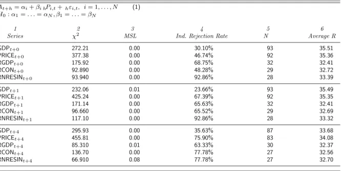
Table 1 presents test results for the null hypothesis of micro-homogeneity for zero-, one-, and four-quarter-ahead forecasts of nominal GDP, real GDP, the GDP deflator, real nonresidential investment, and real consumption. Micro-homogeneity is rejected at marginal significance levels (MSL) of approx-imately 1% or less for all forecast series except the four-quarter-ahead real nonresidential investment series. The marginal significance level for the micro-homogeneity test on the latter series is 0.08. It is interesting to note that in this case the rate of rejection of individual unbiasedness, reported in column four of Table 1, is almost 78%. (For our individual unbiasedness tests we estimate equation (1) using OLS with a Hansen (1982) type correction for M A(k) errors.) Thus, while micro-homogeneity comes close to being an acceptable maintained hypothesis for consensus or pooled regressions with this fore-cast, the explanation appears to be a biased “consensus” in the sense of dictionary definition 2 (see page 3). In fact, the individual rejection rates range from a low of almost 24% to a high of nearly 93%.

(19)

Table 1. Full Sample Micro-homogeneity Tests

At+h=αi+βi hPi,t+hεi,t, i= 1, . . . , N (1)

H0:α1=. . .=αN, β1=. . .=βN

1 2 3 4 5 6

Series χ2 _MSL _{Ind. Rejection Rate} _N _{Average R}

GDPt+0 272.21 0.00 30.10% 93 35.51 PRICEt+0 377.38 0.00 46.74% 92 35.36 RGDPt+0 175.92 0.00 68.75% 32 32.41 RCONt+0 92.890 0.00 48.28% 29 32.72 RNRESINt+0 93.940 0.00 92.86% 28 33.39 GDPt+1 232.06 0.01 23.66% 93 35.49 PRICEt+1 425.24 0.00 67.39% 92 35.35 RGDPt+1 171.14 0.00 65.63% 32 32.41 RCONt+1 96.660 0.00 65.52% 29 32.69 RNRESINt+1 117.10 0.00 92.86% 28 33.32 GDPt+4 295.93 0.00 35.63% 87 33.68 PRICEt+4 455.81 0.00 75.90% 83 34.08 RGDPt+4 85.310 0.01 63.33% 30 32.37 RCONt+4 136.70 0.00 77.78% 27 32.56 RNRESINt+4 66.910 0.08 77.78% 27 32.70

NOTE: Column 1 gives the target series (dependent variable in equation (1)): GDP, RGDP, and PRICE are nominal Gross Domestic Product (GNP prior to 1991:3), real GDP, and the GDP deﬂator; RCON and RNRESIN are real consumption expenditures and real nonresidential investment, respectively. RGDP, RCON, and RNRESIN were not part of the SPF until 1981:3. Column 2 is the value of the Wald test for

H0. Column 3 is the marginal signiﬁcance level of the test in column 2. Column 4 gives the percentage of the individual regression results which produce a rejection of the null of unbiasedness. Column 5 gives the number of survey respondents who meet our minimum response level of 20, and Column 6 gives the average number of responses per individual included in the test.

The statistical and economic significance of these rejections of micro-homogeneity may need qualifica-tion due to two characteristics of the data. First, there is typically a large number of missing observaqualifica-tions per forecaster. Unless these missing observations are random, our tests may suffer from sample selection bias. Second, the pool of forecasters shrinks markedly over the sample period. Thus, our results may be dominated by forecaster performance over the earlier part of the sample period.

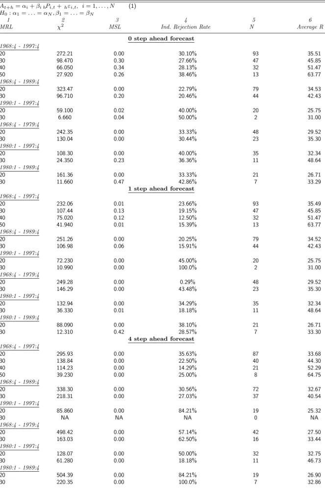
In addressing the first issue, we rule out interpolation methods for filling in missing forecasts. Even if we were to generate predictions of missing forecasts with an iterative method that uses only variables in the forecaster’s information set, we would still be imposing a specific forecast generating process on the individual, then using that pseudo-interpolated data to test his rationality. Clearly, this methodology is unacceptable. Instead, we investigate whether increasing the minimum response level (MRL) from 20 to 30, 40, and 50 observations produces different results. In other words, we eliminate survey respondents with the largest number of missing observations. Tables 2-6 show the results of varying the minimum response level for three different forecast horizons for each of the five variables tested in Table 1.

The thirty-eight (full sample) tests in which minimum response levels are raised to 30, 40, and 50 observations produce only nine nonrejections at the 5% level. Three of these are for the zero-quarter-ahead forecast of nominal GDP and two more are for the one-quarter-zero-quarter-ahead forecast of this variable (see Table 2). Interestingly, the marginal signiﬁcance levels remain at virtually zero for all minimum

(20)

Table 2. Further Micro-homogeneity Tests: Nominal GDP Subsample for Minimum Response Levels

H0:α1=. . .=αN, β1=. . .=βN

1 2 3 4 5 6

MRL χ2 _MSL _{Ind. Rejection Rate} _N _{Average R}

0 step ahead forecast

1968:4 - 1997:4 20 272.21 0.00 30.10% 93 35.51 30 98.470 0.30 27.66% 47 45.85 40 66.050 0.34 28.13% 32 51.47 50 27.920 0.26 38.46% 13 63.77 1968:4 - 1989:4 20 323.47 0.00 22.79% 79 34.53 30 96.710 0.20 20.46% 44 42.43 1990:1 - 1997:4 20 59.100 0.02 40.00% 20 25.75 30 6.660 0.04 50.00% 2 31.00 1968:4 - 1979:4 20 242.35 0.00 33.33% 48 29.52 30 130.04 0.00 30.44% 23 35.30 1980:1 - 1997:4 20 108.30 0.00 40.00% 35 32.34 30 24.350 0.23 36.36% 11 48.64 1980:1 - 1989:4 20 161.36 0.00 33.33% 21 26.71 30 11.660 0.47 42.86% 7 33.29

1968:4 - 1997:4 20 232.06 0.01 23.66% 93 35.49 30 107.44 0.13 19.15% 47 45.85 40 75.020 0.12 12.50% 32 51.47 50 41.940 0.01 15.39% 13 63.77 1968:4 - 1989:4 20 251.26 0.00 20.25% 79 34.52 30 106.98 0.06 15.91% 44 42.43 1990:1 - 1997:4 20 72.230 0.00 45.00% 20 25.75 30 10.990 0.00 100.0% 2 31.00 1968:4 - 1979:4 20 249.28 0.00 0.29% 48 29.52 30 146.29 0.00 43.48% 23 35.30 1980:1 - 1997:4 20 132.94 0.00 34.29% 35 32.34 30 36.330 0.01 18.18% 11 48.64 1980:1 - 1989:4 20 88.090 0.00 38.10% 21 26.71 30 12.310 0.42 28.57% 7 33.30

1968:4 - 1997:4 20 295.93 0.00 35.63% 87 33.68 30 138.84 0.00 22.50% 40 44.30 40 114.23 0.00 14.29% 21 52.29 50 39.230 0.00 25.00% 8 64.75 1968:4 - 1989:4 20 338.30 0.00 30.56% 72 32.67 30 218.31 0.00 27.03% 37 40.54 1990:1 - 1997:4 20 85.860 0.00 84.21% 19 25.32 30 NA NA NA 0 NA 1968:4 - 1979:4 20 498.42 0.00 57.14% 42 27.50 30 163.03 0.00 62.50% 16 33.44 1980:1 - 1997:4 20 128.07 0.00 50.00% 32 32.75 30 61.280 0.00 18.18% 11 46.73 1980:1 - 1989:4 20 504.39 0.00 84.21% 19 26.90 30 220.35 0.00 100.0% 7 32.86

NOTE: Column 1 gives the minimum number of responses for each forecaster (over the sample period under consideration) to be included in the test. Column 2 is the value of the Wald test forH₀. Column 3 is the marginal signiﬁcance level of the test in column 2. Column 4 gives the percentage of individual unbiasedness tests which reject the null of unbiasedness. Column 5 gives the size of the cross section, i.e. the number of individuals who meet the MRL. Column 6 gives the average number of survey responses at each point in time, averaged over the sample period. NA indicates that there were less than two respondents meeting the Minimum Response Level for this sample.

(21)

Table 3. Further Micro-homogeneity Tests: GDP Deﬂator Subsample for Minimum Response Levels

H0:α1=. . .=αN, β1=. . .=βN

1 2 3 4 5 6

MRL χ2 _MSL _{Ind. Rejection Rate} _N _{Average R}

1968:4 - 1997:4 20 377.38 0.00 46.74% 92 35.36 30 223.67 0.00 41.30% 46 45.98 40 190.49 0.00 43.75% 32 51.03 50 59.680 0.00 50.00% 12 64.33 1968:4 - 1989:4 20 310.45 0.00 37.50% 80 34.2 30 210.40 0.00 41.86% 43 42.72 1990:1 - 1997:4 20 101.51 0.00 88.89% 18 25.44 30 3.160 0.21 50.00% 2 31.00 1968:4 - 1979:4 20 268.25 0.00 34.04% 47 29.6 30 168.47 0.00 50.00% 22 35.5 1980:1 - 1997:4 20 320.27 0.00 56.25% 32 32.8 30 55.910 0.00 36.36% 11 47.3 1980:1 - 1989:4 20 244.26 0.00 25.00% 20 26.9 30 28.390 0.00 28.57% 7 32.9

1968:4-1997:4 20 425.24 0.00 67.39% 92 35.35 30 278.10 0.00 67.39% 46 45.98 40 254.18 0.00 75.00% 32 51.03 50 74.050 0.00 75.00% 12 64.33 1968:4 - 1989:4 20 363.45 0.00 63.75% 80 34.19 30 252.82 0.00 65.12% 43 42.72 1990:1 - 1997:4 20 142.05 0.00 72.22% 18 25.44 30 24.940 0.00 50.00% 2 31.00 1968:4 - 1979:4 20 518.57 0.00 59.57% 47 29.6 30 302.52 0.00 86.36% 22 35.5 1980:1 - 1997:4 20 378.10 0.00 59.38% 32 32.8 30 51.740 0.00 45.46% 11 47.27 1980:1 - 1989:4 20 312.12 0.00 40.00% 20 26.9 30 12.230 0.43 57.14% 7 32.86

1968:4-1997:4 20 455.81 0.00 75.90% 83 34.08 30 218.22 0.00 77.50% 40 44.1 40 83.280 0.00 85.00% 20 52.3 50 49.510 0.00 100.00% 8 64 1968:4 - 1989:4 20 320.57 0.00 75.71% 70 32.97 30 204.29 0.00 72.97% 37 40.62 1990:1 - 1997:4 20 453.10 0.00 56.25% 16 25.31 30 NA NA NA 0 NA 1968:4 - 1979:4 20 5.640 1.00 73.81% 42 27.57 30 1446.3 0.00 81.25% 16 33.5 1980:1 - 1997:4 20 438.32 0.00 76.67% 30 32.80 30 60.490 0.00 72.73% 11 45.27 1980:1 - 1989:4 20 428.54 0.00 77.78% 18 26.94 30 21.380 0.05 85.71% 7 32.43

(22)

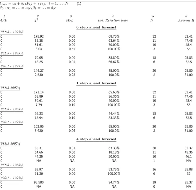
Table 4. Further Micro-homogeneity Tests: Real GDP Subsample for Minimum Response Levels

H0:α1=. . .=αN, β1=. . .=βN

1 2 3 4 5 6

MRL χ2 MSL Ind. Rejection Rate N Average R

1981:3 - 1997:4 20 175.92 0.00 68.75% 32 32.41 30 55.38 0.00 63.64% 11 47.45 40 51.61 0.00 70.00% 10 48.4 50 3.04 0.55 100.00% 3 55 1981:3 - 1989:4 20 79.05 0.00 38.89% 18 25.83 30 18.25 0.05 66.67% 6 32.5 1990:1 - 1997:4 20 144.27 0.00 85.00% 20 25.80 30 2.530 0.28 100.0% 2 31.00

1981:3-1997:4 20 171.14 0.00 65.63% 32 32.41 30 68.89 0.00 36.36% 11 47.45 40 59.61 0.00 40.00% 10 48.4 50 7.79 0.10 100.00% 3 55 1981:3 - 1989:4 20 95.23 0.00 44.44% 18 25.83 30 15.94 0.10 83.33% 6 32.5 1990:1 - 1997:4 20 162.06 0.00 95.00% 20 25.80 30 5.620 0.06 100.0% 2 31.00

1981:3-1997:4 20 85.31 0.01 63.33% 30 32.37 30 54.66 0.00 18.18% 11 45.36 40 44.25 0.00 20.00% 10 46.1 50 NA NA NA 1 NA 1981:3 - 1989:4 20 92.97 0.00 93.75% 16 25.88 30 61.26 0.00 100.00% 6 32 1990:1 - 1997:4 20 93.580 0.00 94.74% 19 25.37 30 NA NA NA 0 NA

(23)

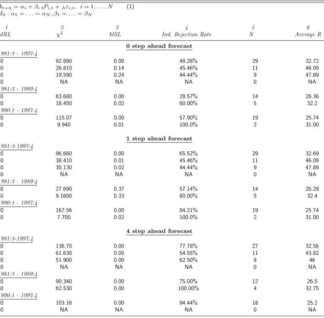
Table 5. Further Micro-homogeneity Tests: Real Consumption Subsample for Minimum Response Levels

H0:α1=. . .=αN, β1=. . .=βN

1 2 3 4 5 6

1981:3 - 1997:4 20 92.890 0.00 48.28% 29 32.72 30 26.810 0.14 45.46% 11 46.09 40 19.590 0.24 44.44% 9 47.89 50 NA NA NA 0 NA 1981:3 - 1989:4 20 63.680 0.00 28.57% 14 26.36 30 18.450 0.02 60.00% 5 32.2 1990:1 - 1997:4 20 115.07 0.00 57.90% 19 25.74 30 9.940 0.01 100.0% 2 31.00

1981:3-1997:4 20 96.660 0.00 65.52% 29 32.69 30 38.410 0.01 45.46% 11 46.09 40 30.130 0.02 44.44% 9 47.89 50 NA NA NA 0 NA 1981:3 - 1989:4 20 27.690 0.37 57.14% 14 26.29 30 9.1600 0.33 80.00% 5 32.4 1990:1 - 1997:4 20 167.56 0.00 84.21% 19 25.74 30 7.700 0.02 100.0% 2 31.00

1981:3-1997:4 20 136.70 0.00 77.78% 27 32.56 30 61.630 0.00 54.55% 11 43.82 40 51.900 0.00 62.50% 8 46 50 NA NA NA 0 NA 1981:3 - 1989:4 20 90.340 0.00 75.00% 12 26.5 30 62.530 0.00 100.00% 4 32.75 1990:1 - 1997:4 20 103.16 0.00 94.44% 18 25.2 30 NA NA NA 0 NA

(24)

Table 6. Further Micro-homogeneity Tests: Real Nonresidential Investment Subsample for Minimum Response Levels

H0:α1=. . .=αN, β1=. . .=βN

1 2 3 4 5 6

1981:3 - 1997:4 20 93.94 0.00 92.86% 28 33.39 30 43.05 0.00 81.82% 11 46.55 40 40.58 0.00 80.00% 10 47.4 50 NA NA NA 0 NA 1981:3 - 1989:4 20 34.75 0.12 85.71% 14 26.5 30 17.43 0.03 100.00% 5 32.6 1990:1 - 1997:4 20 67.710 0.00 94.74% 19 25.80 30 10.100 0.01 100.0% 2 31.00

1981:3 -1997:4 20 117.1 0.00 92.86% 28 33.32 30 60.02 0.00 81.82% 11 46.45 40 56.67 0.00 80.00% 10 47.3 50 NA NA NA 0 NA 1981:3 - 1989:4 20 58.32 0.00 92.86% 14 26.43 30 28.83 0.00 100.0% 5 32.6 1990:1 - 1997:4 20 105.96 0.00 100% 19 25.74 30 9.040 0.01 100.0% 2 31.00

1981:3-1997:4 20 66.91 0.08 77.78% 27 32.7 30 36.87 0.01 63.64% 11 44.09 40 33.68 0.01 70.00% 10 44.7 50 NA NA NA 0 NA 1981:3 - 1989:4 20 18.23 0.79 61.54% 13 26 30 8.22 0.41 60.00% 5 32 1990:1 - 1997:4 20 59.220 0.01 100.0% 18 25.28 30 NA NA NA 0 NA

(25)

response levels for the zero- and one-quarter-ahead forecast of the GDP deﬂator reported in Table 3. MSLs rise to nonrejection levels only for the 50 response level for real GDP in Table 4, where the number of respondents drops to only three. Thus, when there is a response level of 30 or more, there is less evidence against micro-homogeneity for forecasts of nominal GDP than for the deﬂator or real GDP.

One possible explanation of these results is that forecasts of nominal GDP are more uniformly un-biased than forecasts of either component factor, due to oﬀsetting forecast errors in each factor. This conjecture is borne out by results of the individual unbiasedness tests. With a minimum response level of 30 or more, the percentage of rejections reported in column four ranges from 28% to 38% for zero-quarter-ahead nominal GDP (Table 2), 41% to 50% for the zero-zero-quarter-ahead deﬂator (Table 3), and 64% to 100% for zero-quarter-ahead real GDP (Table 4). This pattern is also present in the other forecast horizons of these variables.

To summarize our ﬁndings on the eﬀect of missing observations, we conclude that, except for short horizon forecasts of nominal GDP, eliminating forecasters who respond less frequently does not result in a more homogeneous sample of forecasts or an increase in nonrejection of micro-homogeneity tests.

The second possible drawback to the use of the Survey of Professional Forecasters’ data is that the cross-sectional dimension of the survey has shrunk steadily since the survey began in 1968:4. The shrinking number of survey responses combined with individual missing observations can result in a very small number of observations at any given point in time near the end of the sample period. Figure 3.1 below illustrates the size of the cross section for the one-quarter-ahead deﬂator forecast at each point in time from 1968:4 to 1997:4. The cross section is counted after ﬁrst excluding individuals who do not meet the minimum response levels 20, 30, 40, and 50 forecasts over the entire sample period.

Are our test results driven by a disproportionate number of observations in the earlier part of the sample period? First, note that the higher we set the minimum response level, the smaller the decline in eligible forecasters over time. Thus, increasing the minimum response level serves two purposes: it not only reduces the number of missing observations per forecaster, but also signiﬁcantly attenuates the decline in the total number of forecasters over the sample period.

To investigate any remaining effects of the decline in the number of eligible forecasters on our test results, we begin by determining the dates at which the number of survey respondents falls below various thresholds, assuming a minimum response level of 20. The number of eligible survey respondents falls below 25 for the first time in 1980:1 and below 15 for the first time in 1990:1. These two dates determine

(26)

0 10 20 30 40 50

60 Figure 3.1: Cross-Sectional Sample Size

1968:4 1972:4 1976:4 1980:4 1984:4 1988:4 1992:4 1996:4 MRL = 20 MRL = 30 ❜ ❜ ❜❜❜❜❜ ❜❜ ❜❜ ❜❜❜❜ ❜❜❜ ❜ ❜❜ ❜ ❜ ❜ ❜❜❜❜ ❜❜❜❜❜❜❜❜ ❜ ❜ ❜ ❜❜❜❜❜❜❜❜_❜❜❜ ❜❜ ❜❜❜❜❜❜❜❜❜❜❜❜❜❜❜❜❜❜❜❜❜❜❜❜_{❜❜❜❜❜❜❜} ❜❜❜ ❜❜❜❜❜_{❜❜❜❜❜❜❜❜❜❜❜❜❜❜❜❜❜❜❜} ❜❜❜❜❜❜❜ ❜ MRL = 40 MRL = 50 ✸✸ ✸✸✸✸✸✸✸✸✸✸✸✸✸✸✸✸✸✸✸✸✸✸✸✸✸✸✸✸✸✸✸✸✸✸✸_✸✸_✸✸✸✸✸✸✸_✸✸✸✸_✸✸✸✸✸✸✸✸✸✸✸✸ ✸✸ ✸✸✸✸✸✸✸✸✸✸✸✸✸✸✸ ✸✸✸✸✸✸✸✸✸✸✸✸✸✸✸✸✸✸✸✸✸✸✸✸✸✸✸✸✸✸✸_{✸✸✸✸✸✸✸} ✸

the break points for our subsample tests of nominal GDP and the deﬂator. For these variables, we conduct tests for all possible subsamples: 1968:4-1989:4, 1990:1-1997:4, 1968:4-1979:4, 1980:1-1997:4, and 1980:1-1989:4. For forecasts of real GDP, consumption, and nonresidential investment, which were introduced in the survey in 1981:3, we conduct subsample tests for 1981:3-1989:4 and 1990:1-1997:4. The results are presented in Tables 2-6.

Full sample testing over all variables, horizons, and minimum response levels produces forty-three rejections and ten nonrejections. In general, the nonrejections appear to be associated with shorter forecast horizons, possibly more forecast experience (i.e., a higher minimum response level), and the decade of the 1980s. Recall that, in the full sample, the variables producing the most nonrejections of micro-homogeneity are nominal GDP at zero and one-quarter-ahead horizons, for minimum response levels of 30, 40 and 50. Subsample tests for zero-step-ahead nominal GDP forecasts produce nonrejec-tions (for a minimum response level of 30) in all periods except the earliest (1968:4-1979:4). For the one-step-ahead forecast of nominal GDP, rejections occur in the 1980:1-1997:4 subperiod as well as the earliest subperiod.

Of the forty-three full sample rejections, twenty-six also satisfy minimum response levels of 20 or 30 in at least some subsamples. For these variables, we examine robustness of the full-sample rejections by conducting tests on these eligible subsamples. The 77 subsample tests produce only ten nonrejections. Interestingly, six out of the ten nonrejections are for the decade of the 1980s; the 1990:1-1997:4 subperiod produces three nonrejections and twenty-two rejections. Each of the three nonrejections has an eligible

(27)

cross section of only two forecasters. Thus, full sample rejections of micro-homogeneity do not appear to be an artifact of the overall decline in the number of forecasters in the 1990s. Therefore, once we specify a minimum response level, the nonrejections of micro-homogeneity for the full sample appear to occur in spite of, not because of, the steady decline in eligible forecasters over time.

In addition to our tests of the micro-homogeneity hypothesis, the fourth column of each table reports the percentage of individual unbiasedness tests which reject at the 5% level. We find widespread rejection of the unbiasedness hypothesis at the individual level. For the full sample results reported in Table 1, the percentage of rejections range from a low of 23.7% for one-step-ahead nominal GDP forecasts to a high of 92.9% for zero- and one-step-ahead real nonresidential investment forecasts. Our findings are consistent with the results of other researchers. For forecasts of changes in the GDP deflator, Zarnowitz (1985) rejected the unbiasedness hypothesis (at the 5% level) in over 26% of the contemporaneous forecasts, more than 46% of the one-quarter-ahead forecasts, and 58% of the four-quarter-ahead forecasts. For contemporaneous, one-quarter-ahead, and four-quarter-ahead forecasts of the changes in nominal GDP, the rejection rates were greater than twelve, ten, and eleven percent respectively. In an earlier paper, Bonham and Cohen (1992) rejected the null hypothesis of unbiasedness at the 5% significance level for 40% of the eighty survey respondents in their sample of contemporaneous price forecasts. The corresponding fraction of rejections for the one-quarter-ahead forecasts was 50%.

These results are consistent with our finding of widespread rejection of micro-homogeneity. A sig-nificant number of individual respondents to the Survey of Professional Forecasters do not produce unbiased predictions of the five series studied here, and the micro-homogeneity tests show that their forecasts differ systematically. Furthermore, rejection of micro-homogeneity suggests that parameter estimates in consensus unbiasedness regressions are likely to be inconsistent or lead to false acceptance of the unbiasedness hypothesis. Therefore pooled estimates may suffer from heterogeneity bias and thus do not represent a viable alternative to consensus estimates.

4. CONCLUSIONS AND EXTENSIONS

This paper investigates the usefulness of panels of survey forecasts for testing the unbiasedness prop-erty of the Rational Expectations Hypothesis. Survey data may be used in individual, consensus, or pooled regression speciﬁcations. Although these data are most commonly used in “consensus” form, a number of authors have criticized this speciﬁcation for introducing at least two kinds of bias. Figlewski and Wachtel (1983) argued that aggregation of individual-rational forecasts may lead to parameter

(28)

estimates which are inconsistent due to private information bias, and Keane and Runkle (1990) argued that averaging individual-irrational forecasts may lead to false acceptance of the unbiasedness hypoth-esis. The literature has turned to the pooled speciﬁcation in an attempt to avoid these two sources of bias. However, Zarnowitz (1985) argued that pooled unbiasedness parameters are inconsistent, due to constant cross-sectional realizations.

We show that the criticisms of consensus and pooled speciﬁcations are only valid when forecasts and realizations are stationary. When these series are integrated and cointegrated, the criticisms break down asymptotically provided micro-homogeneity obtains. Thus, micro-homogeneity is a crucial condition for the validity of both consensus and pooled tests of the unbiasedness hypothesis. Because micro-heterogeneity is a source of bias in both the consensus and pooled speciﬁcations, the attempt to avoid aggregation problems by pooling is misguided. While a few authors have conducted tests for poolability, we are unaware of any work which recognizes this close relationship between the presence of aggregation bias in consensus regressions and heterogeneity bias in pooled regressions.

To conduct such tests we extend Zellner’s (1962a) micro-homogeneity test to the case of Generalized Method of Moments (GMM) estimation and adapt a weighting matrix suggested by Keane and Runkle (1990), which accounts for the possibility that forecast errors follow moving average processes both individually and across respondents. We show that micro-homogeneity does not hold for forty-three out of fifty-three or eighty-one percent of the SPF’s forecasts of nominal GDP, the GDP deflator, real GDP, real consumption expenditures, and real nonresidential investment over various forecast horizons, sample periods, and minimum response levels. Thus, at least for these forecasts, unbiasedness should only be tested at the individual level. The ten nonrejections of micro-homogeneity tend to be associated with shorter forecast horizons, forecaster experience (i.e. a higher minimum response level), and the decade of the 1980s. (Five of the nine nonrejections are for various tests of nominal GDP forecasts.) Therefore, for these forecasts, consensus and pooled specifications may be used in testing the unbiasedness hypothesis. Since individual-rational expectations imply homogeneity in the panel, rejection of micro-homogeneity implies some degree of bias in the panel forecasts. Thus, we expect that individual un-biasedness tests will also produce rejections. Indeed, we reject individual unun-biasedness in anywhere from 24% to nearly 93% of our individual regressions. Studies by Zarnowitz (1985), Batchelor and Dua (1991), and Bonham and Cohen (1992) confirm our findings and provide evidence of both widespread bias in professional forecasts and considerable micro-heterogeneity. These findings imply that agents make use of different private and/or public information when forming their predictions. Therefore,