Challenges in Large-Scale Machine Learning Systems: Security and Correctness

(1)

University of South Carolina University of South Carolina

Scholar Commons

Theses and Dissertations Fall 2019

Challenges in Large-Scale Machine Learning Systems: Security

and Correctness

Emad Alsuwat

Follow this and additional works at: https://scholarcommons.sc.edu/etd

Part of the Computer Sciences Commons, and the Engineering Commons Recommended Citation

Recommended Citation

Alsuwat, E.(2019). Challenges in Large-Scale Machine Learning Systems: Security and Correctness. (Doctoral dissertation). Retrieved from https://scholarcommons.sc.edu/etd/5596

This Open Access Dissertation is brought to you by Scholar Commons. It has been accepted for inclusion in Theses and Dissertations by an authorized administrator of Scholar Commons. For more information, please contact [email protected].

(2)

CHALLENGES INLARGE-SCALE MACHINELEARNINGSYSTEMS: SECURITY AND

CORRECTNESS

by Emad Alsuwat

Bachelor of Computer Science Taif University, 2008

Master of Science

University of South Carolina, 2014

Submitted in Partial Fulﬁllment of the Requirements for the Degree of Doctor of Philosophy in

Computer Science and Engineering College of Engineering and Computing

University of South Carolina 2019

Accepted by:

Csilla Farkas, Major Professor Marco Valtorta, Major Professor

John Rose, Committee Member Chin-Tser Huang, Committee Member

Linyuan Lu, Committee Member

(3)

c

(4)

D

EDICATION

I am dedicating this dissertation to my beloved family. This work could not be done with you. I am very thankful for all of your support and encouragement along the way.

(5)

A

CKNOWLEDGMENTS

First and foremost I express my sincere gratitude for my advisors Prof. Csilla Farkas and Prof. Marco Valtorta. It has been an honor to be their PhD student. I am very thankful for their motivation, immense knowledge, and continuous support. I appreciate all the contributions of time and ideas to make my PhD dissertation experience productive and stimulating.

Besides my advisors, I would like to thank the rest of my dissertation committee mem-bers, Prof. John Rose, Prof. Chin-Tser Huang, and Prof. Linyuan Lu, for their insightful comments and encouragement.

I would like to thank my family for all their unlimited encouragement and love. I would like to sincerely thank my parents who raised me with a love of science and for providing me the support I need. I also would like to thank my brothers, sisters, wife and son for supporting me spiritually throughout my life.

Last but not the least, I would like to thank my friends for all their love and true friend-ship. My time at the University of South Carolina was made enjoyable in large part due to the many friends that became a part of my life. I am grateful for time spent with them and grateful for unforgettable memories.

(6)

A

BSTRACT

In this research, we address the impact of data integrity on machine learning algorithms. We study how an adversary could corrupt Bayesian network structure learning algorithms by inserting contaminated data items. We investigate the resilience of two commonly used Bayesian network structure learning algorithms, namely the PC and LCD algorithms, against data poisoning attacks that aim to corrupt the learned Bayesian network model.

Data poisoning attacks are one of the most important emerging security threats against machine learning systems. These attacks aim to corrupt machine learning models by con-taminating datasets in the training phase. The lack of resilience of Bayesian network struc-ture learning algorithms against such attacks leads to inaccuracies of the learned network structure.

In this dissertation, we propose two subclasses of data poisoning attacks against Bayes-ian networks structure learning algorithms: (1) Model invalidation attacks when an ad-versary poisons the training dataset such that the Bayesian model will be invalid, and (2) Targeted change attacks when an adversary poisons the training dataset to achieve a specific change in the structure. We also define a novel measure of the strengths of links between variables in discrete Bayesian networks. We use this measure to find vulnera-ble sub-structure of the Bayesian network model. We use our link strength measure to find the easiest links to break and the most believable links to add to the Bayesian net-work model. In addition to one-step attacks, we define long-duration (multi-step) data poisoning attacks when a malicious attacker attempts to send contaminated cases over a period of time. We propose to use the distance measure between Bayesian network models and the value of data conflict to detect data poisoning attacks. We propose a 2-layered

(7)

framework that detects both traditional one-step and sophisticated long-duration data poi-soning attacks. Layer 1 enforces “reject on negative impacts” detection; i.e., input that changes the Bayesian network model is labeled potentially malicious. Layer 2 aims to detect long-duration attacks; i.e., observations in the incoming data that conﬂict with the original Bayesian model.

Our empirical results show that Bayesian networks are not robust against data poisoning attacks. However, our framework can be used to detect and mitigate such threats.

(8)

T

ABLE OF

C

ONTENTS

DEDICATION . . . iii

ACKNOWLEDGMENTS . . . iv

ABSTRACT . . . v

LIST OFTABLES . . . xi

LIST OFFIGURES . . . xiv

CHAPTER 1 INTRODUCTION . . . 1

1.1 Introduction . . . 1

1.2 Running Example and Test Setup . . . 4

1.3 Research Tasks . . . 7

1.4 Dissertation Outline . . . 12

CHAPTER 2 LITERATURE REVIEW . . . 14

2.1 Bayesian Networks . . . 14

2.2 The Notion of D-separation . . . 15

2.3 Structure Learning in Bayesian Networks . . . 17

2.4 Prior to Posterior Updating . . . 19

(9)

2.6 Adversarial Machine Learning . . . 22

2.7 Defenses and Countermeasures for Data Poisoning attacks . . . 23

CHAPTER 3 OVERVIEW OF THEPROPOSED SYSTEM . . . 26

3.1 Overview of Adversarial Attacks Against Bayesian Network Models . . . . 26

3.2 Threat Model for Data Poisoning Attacks Against the PC Algorithm . . . . 26

CHAPTER 4 LINK STRENGTHS FROM DATA INDISCRETE BAYESIANNETWORKS 28 4.1 Introduction . . . 28

4.2 Deﬁnition of the Proposed Link Strengths Measure (L_S) . . . 28

4.3 Explanation . . . 29

4.4 Interpretation . . . 30

4.5 Practical usages . . . 30

4.6 Experimental Results . . . 31

4.7 Comparison with Previous Link Strength Measures . . . 31

CHAPTER 5 MODELINVALIDATION ATTACKS . . . 34

5.1 Overview of Model Invalidation Attacks . . . 34

5.2 Model Invalidation Attacks Based on the Notion of D-separation . . . 35

5.3 Model Invalidation Attacks Based on Marginal Independence Tests . . . 40

5.4 Empirical Results for Model Invalidation Attacks Based on the Notion of D-separation . . . 46

5.5 Empirical Results for Model Invalidation Attacks Based on Marginal Independence Tests . . . 47

(10)

6.1 Overview of Targeted Change Attacks . . . 53

6.2 Empirical Results for Targeted Change Attacks . . . 55

CHAPTER 7 ADVERSARIAL ATTACKSAGAINST THELCD ALGORITHM . . . . 58

7.2 Empirical Results . . . 59

7.3 Empirical Results of Model Invalidation Attacks Based on the Notion of D-separation . . . 60

7.4 Empirical Results of Model Invalidation Attacks Based on Marginal Independence Tests . . . 60

7.5 Which algorithm is more robust to data poisoning attacks: The PC Al-gorithm or the LCD AlAl-gorithm? . . . 63

CHAPTER 8 LONG-DURATIONDATAPOISONINGATTACKS . . . 65

CHAPTER 9 DETECTINGADVERSARIALATTACKS IN THECONTEXT OFBAYESIAN NETWORKS . . . 72

9.2 Problem Setting . . . 73

9.3 Framework for Detecting Data Poisoning Attacks . . . 78

CHAPTER 10 CONCLUSION AND FUTURE WORK . . . 84

10.1 Conclusion . . . 84

(11)

BIBLIOGRAPHY . . . 86

APPENDIXA COMPUTATIONS OFPOSTERIOR DISTRIBUTIONS . . . 93

A.1 Edges of the Chest Clinic Network . . . 93

APPENDIXB COMPUTATIONS OFLINK STRENGTHMEASURE (L_S) . . . 110

B.1 Using L_S on the Chest Clinic Network . . . 110

APPENDIXC COMPUTATION OFMUTUALINFORMATIONLINK STRENGTH . . 113

C.1 Experimental Results . . . 113

APPENDIXD CORRUPTED CASESUSED TO ADD LINKS TO CHESTCLINIC NETWORK . . . 127

(12)

L

IST OF

T

ABLES

Table 1.1 Selected tuples from the original datasetDB1 . . . 2

Table 1.2 DB′₁, which is equal toDB1except for three changes in bold font . . . . 3

Table 2.1 Conditional probability tables for a simple BN for modeling a travel-ing activity . . . 16

Table 4.1 A contingency table for two discrete variablesV ariable1andV ariable2 withiandj states, respectively. . . 29

Table 4.2 Posterior distributions for the Chest Clinic Network. . . 31

Table 4.3 Using L_S and MI to compute link strength of the original Chest Clinic Network . . . 33

Table 5.1 Posterior distributions for the Chest Clinic Network. . . 49

Table 5.2 The result of usingL_Sto rankB1edges from the weakest to the strongest. 51 Table 5.3 Posterior distributions for the set of edgesQ. . . 52

Table 5.4 L_Sresults. . . 52

Table 7.1 Summary of the required number of corrupt cases to contaminated the datasetDB1. . . 63

Table 8.1 Results of long-duration data poisoning attacks againstDSv_{. . . 71}

Table 9.1 Notations . . . 77

Table 9.2 Results of using FLoD to detect one-step data poisoning attacks. . . 81

(13)

Table A.1 The contingency table of the observed counts of P(B |S) . . . 94

Table A.2 The contingency table of the observed counts of P(L|S) . . . 96

Table A.3 The contingency table of the observed counts of P(T |A) . . . 98

Table A.4 The contingency table of the observed counts of P(E |T) . . . 100

Table A.5 The contingency table of the observed counts of P(E |L) . . . 102

Table A.6 The contingency table of the observed counts of P(X |E) . . . 104

Table A.7 The contingency table of the observed counts of P(D|E) . . . 106

Table A.8 The contingency table of the observed counts of P(D|B) . . . 108

Table B.1 Posterior distributions for the Chest Clinic Network. . . 110

Table C.1 The conditional probability for variableT . . . 113

Table C.2 The joint probability for variablesT andA . . . 114

Table C.3 The conditional probability for variableB . . . 115

Table C.4 The joint probability for variableB andS . . . 116

Table C.5 The conditional probability for variableL . . . 117

Table C.6 The joint probability for variablesLandS. . . 117

Table C.7 The conditional probability for variableE . . . 118

Table C.8 The joint probability for variablesE,T andL . . . 120

Table C.9 The joint probability for variablesE andT . . . 120

Table C.10 The joint probability for variablesE andL . . . 121

Table C.11 The conditional probability for variableD . . . 122

Table C.12 The joint probability for variablesD,E andB . . . 123

(14)

Table C.14 The joint probability for variablesDandE . . . 124

Table C.15 The conditional probability for variableX . . . 125

Table C.16 The joint probability for variablesX andE . . . 126

Table D.1 74 cases to be added toDB1to introduce the linkD−S . . . 127

Table D.2 13 cases to be added toDB1to introduce the linkB−L . . . 130

Table D.3 3 cases to be added toDB1 to introduce the linkA−E . . . 131

Table D.4 8 cases to be added toDB1 to break the unshielded colliderE . . . 131

Table D.5 17 cases to be added to DB1 to change the directions of the triple T −E−L . . . 132

(15)

L

IST OF

F

IGURES

Figure 1.1 The Bayesian learning outcome when feedingDB1to the PC algorithm 2

Figure 1.2 The Bayesian learning outcome when feedingDB1to the PC algorithm 3

Figure 1.3 The original Chest Clinic Network. . . 6

Figure 1.4 B1, the result of feedingDB1 to the PC algorithm with signiﬁcance level at0.05 . . . 6

Figure 1.5 The Bayesian network modelB3, the result of feedingDB1 to the LCD algorithm with signiﬁcance level at0.05 . . . 7

Figure 2.1 A simple BN for modeling a traveling activity . . . 15

Figure 2.2 An example of a serial Connection . . . 16

Figure 2.3 An example of a diverging connection . . . 16

Figure 2.4 An example of a converging connection . . . 17

Figure 3.1 Overview of how data poisoning attacks against Bayesian network structure learning algorithms work. . . 27

Figure 4.1 Results ofL_S on the Chest Clinic Network. . . 32

Figure 5.1 Three cases for the proof of Theorem 5.1. . . 35

Figure 5.2 Introducing a new converging connection in the tripleD−B −S. . . . 47

Figure 5.3 Introducing a new converging connection in the tripleB −S−L. . . . 48

Figure 5.4 Introducing a new converging connection in the tripleS−L−E. . . . 48

(16)

Figure 5.6 Breaking an existing converging connection in the tripleT −E−L. . . 49

Figure 5.7 The result of using17cases to break the v-structureT →E ←L. . . . 49

Figure 5.8 Results ofL_S on the learned model by the PC algorithmB1. . . 50

Figure 5.9 The result of removing the weakest link inB1,A→T . . . 51

Figure 5.10 The result of adding the most believable link toB1,B →L. . . 51

Figure 6.1 A targeted attack against modelB1 . . . 56

Figure 6.2 The modelB1after achievingstep 1(deletingS →L) . . . 56

Figure 6.3 The modelB1after achieving thetwo stepsof the targeted attack . . . . 57

Figure 7.1 The result of adding the edgeD−Sto the Bayesian modelB3 . . . 61

Figure 7.2 The result of adding the edgeB−Lto the Bayesian modelB3 . . . 61

Figure 7.3 The result of adding the edgeS−Eto the Bayesian modelB3 . . . 61

Figure 7.4 The result of adding the edgeA−Eto the Bayesian modelB3 . . . 62

Figure 7.5 The result of adding the edgeT −Lto the Bayesian modelB3 . . . 62

Figure 7.6 The result of deleting the weakest edge A−T from the Bayesian modelB3 . . . 63

Figure 7.7 The result of adding the most believable yet incorrect edgeD−S to the Bayesian modelB3 . . . 63

Figure 9.1 Framework . . . 80

Figure 9.2 The result of usingSLoDto detect a long-duration attack that aims to introduce the linkD → S in the Chest Clinic dataset,DSv. We present the case number inDS_tcas the variable on the X-axis and the value of our conﬂict measureConf(c, B1)as the variable on the Y-axis. A case is incompatible (conﬂicting) with the validated model B1 ifConf(c, B1)>0. . . 83

(17)

Figure A.2 Beta Distribution for P(L|S) . . . 97

Figure A.3 Beta Distribution for P(T |A) . . . 99

Figure A.4 Beta Distribution for P(E |T) . . . 101

Figure A.5 Beta Distribution for P(E |L) . . . 103

Figure A.6 Beta Distribution for P(X |E) . . . 105

Figure A.7 Beta Distribution for P(D|E) . . . 107

(18)

C

HAPTER

1 I

NTRODUCTION

1.1 INTRODUCTION

Machine learning algorithms, including Bayesian Network algorithms, are not secure against adversarial attacks. A machine learning algorithm is asecure learning algorithmif it func-tions well in adversarial environments [10]. Recently, several researchers addressed the problem of attacking machine learning algorithms [10, 16, 63, 50]. Data poisoning at-tacks are considered one of the most important emerging security threats against machine learning systems [43]. These attacks aim to corrupt the machine learning model by con-taminating the data in the training phase.

Data poisoning attacks against Support Vector Machines (SVMs) [16, 66, 67, 47, 42, 19, 32] and Neural Networks (NNs) [69] have been studied extensively. However, we found no research on evaluating the vulnerabilities of Bayesian network learning algo-rithms against adversarial attacks.

In this dissertation, we investigate data poisoning attacks against Bayesian network algorithms. We study two classes of attacks against Bayesian network structure learning algorithms: model invalidation attacks and targeted change attacks. For model invalidation attacks, an adversary poisons the training dataset such that the learned Bayesian model will be invalid. For targeted change attacks, an adversary poisons the training dataset to achieve a particular goal, such as masking or adding a link in a Bayesian network model [6] [8] [9]. For example, assume thatDB1 is a learning dataset, and the modelB1 is the learning

(19)

Table 1.1: Selected tuples from the original datasetDB1

X B D A S L T E

No Yes No Yes No No Yes No

No No No No No No Yes No

Yes No Yes No No No No No

No No No No No Yes No No

No No No No No No Yes No

No Yes No Yes No No Yes Yes . . .

. . . . . .

No No Yes No No Yes No No No No No Yes No No Yes No

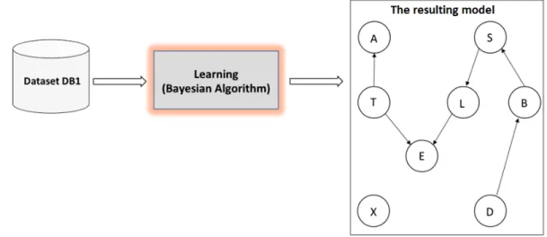
the learning outcome when feedingDB1to the PC learning algorithm.

Figure 1.1: The Bayesian learning outcome when feedingDB1 to the PC algorithm

Table 1.1 shows a sample of the originalDB1. Assume that the attacker has access to

DB1. If the attacker wants to corrupt the learned model, he/she may modify the data in

DB1. Table 1.2 shows the datasetDB

′

1 with changes of three data items.

Using the new corrupted datasetDB₁′, the learned Bayesian model is as shown in Fig-ure 1.2. In this model (FigFig-ure 1.2), the link from nodeT to nodeAis missing. Clearly, the attacker succeeded in corrupting the structure of the model.

(20)

Table 1.2: DB₁′, which is equal toDB1 except for three changes in bold font X B D A S L T E No Yes No No No No Yes No No No No No No No Yes No Yes No Yes No No No No No No No No No No Yes No No No No No No No No Yes No

No Yes No Yes No No No Yes . . .

. . . . . .

No No Yes No No Yes No No

No No No Yes No No No No

Figure 1.2: The Bayesian learning outcome when feedingDB1 to the PC algorithm

In this dissertation, we also aim to deﬁne machine learning security best practices with the goal of detecting and preventing these types of attacks. Succeeding in building a good defensive measure against these attacks will advance the research ﬁeld of adversarial ma-chine learning and minimize the risk of data poisoning attacks, which is one of the most important emerging security threats.

The main contributions of this dissertation are as follows: we propose two subclasses of data poisoning attacks against Bayesian network structure learning algorithms: (1) Model invalidation attacks when an adversary poisons the training dataset such that the Bayesian

(21)

network model will be invalid, and (2) Targeted change attacks when an adversary poisons the training dataset to achieve a specific change in the learned structure. We define a novel measure of strengths of links between variables in discrete Bayesian networks. We show how to use this measure to evaluate the robustness of Bayesian network models. That is, we use our link strength measure to find the easiest links to break and the most believable links to add to a given Bayesian network model. In addition to traditional one-step data poisoning attacks, we define long-duration data poisoning attacks when an attacker may spread the malicious workload over a period of time. We propose a 2-layered framework to detect data poisoning attacks against Bayesian network structure learning algorithms. Our 2-layered framework detects both one-step and long-duration data poisoning attacks. We use the distance between Bayesian network models,B1 andB2, denoted asds(B1, B2), to

detect malicious data input (Equation 2.3) for one-step attacks. For long-duration attacks, we use the value of data conﬂict (Equation 2.5) to detect potentially poisoned data. Our framework relies on ofﬂine analysis to validate the potentially malicious datasets.

We implement our approaches and apply them to the Chest Clinic Network. Our empir-ical results show that Bayesian network structure learning algorithms are vulnerable to data poisoning attacks. Moreover, even a small number of adversarial data may be sufﬁcient to corrupt the model. We show the effectiveness of our framework to detect both one-step and long-duration attacks. Our results indicate that the distance measure ds(B1, B2)

(Equa-tion 2.3) and the conﬂict measure Conf(c, B1) (Equation 2.5) are sensitive to poisoned

data.

1.2 RUNNINGEXAMPLE ANDTESTSETUP

In this dissertation, we demonstrate the robustness of Bayesian network structure learning algorithms against the proposed data poisoning attacks. We also develop detection methods against such adversarial attacks. The feasibility of such attacks and detection methods is investigated through empirical results on the Chest Clinic Network [34].

(22)

To set up the test, we ﬁrst present a canonical Bayesian network, the Chest Clinic Network (also called Visit to Asia network). The Chest Clinic Network was created by Lauritzen and Spielgelhalter in 1988 [34]. As shown in Figure 1.3, Visit to Asia is a simple, ﬁctitious network that could be used at a clinic to diagnose arriving patients. It consists of 8 nodes and 8 edges. The nodes are as follows:

1) (node A)shows whether the patient lately visited Asia; 2) (node S)shows if the patient is a smoker;

3) (node T)shows if the patient has Tuberculosis; 4) (node L)shows if the patient has lung cancer; 5) (node B)shows if the patient has Bronchitis;

6) (node E)shows if the patient has either Tuberculosis or lung cancer; 7) (node X)shows whether the patient X-ray is abnormal; and

8) (node D)shows if the patient has Dyspnea.

The edges indicate the causal relations between the nodes. A simple example for a causal relation is: Visiting Asia may cause Tuberculosis and so on. Lauritzen and Spielgelhalter’s complete description of this simple network is as follows:

Shortness-of-breath (dyspnoea) may be due to tuberculosis, lung cancer, or bronchitis, or none of them, or more than one of them. A recent visit to Asia increases the chances of tuberculosis, while smoking is known to be a risk factor for both lung cancer and bronchitis. The results of a single chest X-ray do not discriminate between lung cancer and tuberculosis, as neither does the presence or absence of dyspnoea [34].

(23)

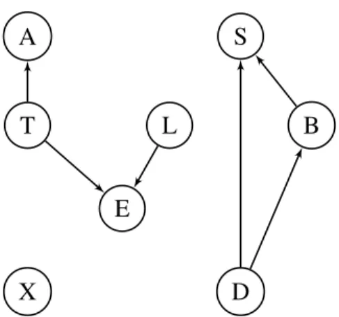
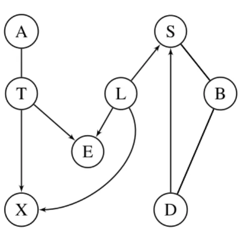
We implemented the Chest Clinic Network using HuginTM Research 8.1. Then we simulated dataset of 10,000 cases for our experiments by using HuginTM case genera-tor [38, 49]. We call this dataset DB1. Using the PC algorithm on dataset DB1 with 0.05signiﬁcance setting [38], the resulting structure is given in Figure 1.4. Also, Using the LCD algorithm on datasetDB1with0.05signiﬁcance setting [38], the resulting

struc-ture is given in Figure 1.5. While the networks that were learned by the PC and LCD algorithms belong to different Markov equivalence classes than the original Chest Clinic Network, we will use these networks of Figure 1.4 and Figure 1.5 as the starting points of our experiments.

A S

T L B

E

X D

Figure 1.3: The original Chest Clinic Network.

A S

T L B

E

X D

Figure 1.4: B1, the result of feeding DB1 to the PC algorithm with signiﬁcance level at 0.05

(24)

A S

T L B

E

X D

Figure 1.5: The Bayesian network modelB3, the result of feedingDB1 to the LCD

algo-rithm with signiﬁcance level at0.05

It is important to point out that proposed attacks require the existence of a triple in the attacked Bayesian network model and their ease depends on the link strength measure. Insertion or removal of edges in Bayesian networks is restricted by the topology of the model. For example, for shielding a collider, it is necessary to insert an edge between its parents. However, attacks must not violate the requirement that a Bayesian network is deﬁne as a directed acyclic graph. For example, we cannot insert a new edge fromE to S in the model B1 because it would create a cycle. We will use link strength measures

as a security analysis tool for checking the feasibility of the proposed attacks. Another important note is that proposed data poisoning attacks may inﬂuence the decision making process that uses the poisoned model. For example, an attack on the Chest Clinic Network that aims to mask the edge from smoking, node S, to lung cancer, node L, may impact decision making as the decision maker will no longer believe that smoking is a cause of lung cancer. However, analysis of the impact on high-level (abstract) decision making needs further evaluation. It is not the purpose of this dissertation.

1.3 RESEARCHTASKS

(25)

1. Adversarial Attacks against Bayesian Networks - the goal of this research task is to determine if adversarial attacks against Bayesian networks exist. The following subtasks have been completed:

a) Research publications.

b) Deﬁne two subclasses of data poisoning attacks against Bayesian network mod-els.

c) Develop the threat model. • Completed: 1a, 1b, 1c • Remaining: None

• Emad Alsuwat, Marco Valtorta, and Csilla Farkas,Bayesian structure learning attacks, Tech. report, University of South Carolina, SC, USA, 2018.

2. Link Strength Measure in Discrete Bayesian Networks - the goal of this research task is to deﬁne a new link strength measure between random variables in discrete Bayesian networks. The following subtasks have been completed:

a) Research and study existing link strength measures. b) Propose a new link strength measure deﬁnition. c) Test our proposed deﬁnition of link strength.

d) Implement our link strength measure and establish the results. e) Compare our link strength measure with existing measures.

• Completed: 2a, 2b, 2c, 2d, 2e • Remaining: None

• Emad Alsuwat, Marco Valtorta, and Csilla Farkas,How to generate the network you want with the pc learning algorithm, Proceedings of the 11th Workshop on Uncertainty Processing (WUPES’18), 2018, pp. 1 – 12.

(26)

3. Adversarial Attacks against Bayesian Networks - the goal of this research task is to study model invalidation attacks based on the notion of d-separation. The following subtasks have been completed:

a) Develop model invalidation attacks based on the notion of d-separation - creating a new converging connection (v-structure).

b) Develop an algorithm for attacks based on creating a new converging connection (v-structure).

c) Implement the algorithm and establish the results.

d) Develop model invalidation attacks based on the notion of d-separation - breaking an existing converging connection (v-structure).

e) Develop an algorithm for attacks based on breaking an existing converging con-nection (v-structure).

f) Implement the algorithm and establish the results. • Completed: 3a, 3b, 3c, 3d, 3e, 3f

• Remaining: None

• Emad Alsuwat, Hatim Alsuwat, Marco Valtorta, and Csilla Farkas, Cyber at-tacks against the pc learning algorithm, 2nd International Workshop on A.I. in Security, 2018, pp. 19 – 35.

4. Adversarial Attacks against Bayesian Networks - the goal of this research task is to study model invalidation attacks based on marginal independence tests. The follow-ing subtasks have been completed:

a) Develop model invalidation attacks based on marginal independence tests - re-moving the weakest edge.

(27)

b) Develop an algorithm for attacks based on removing the weakest edge. c) Implement the algorithm and establish the results.

d) Develop model invalidation attacks based on marginal independence tests - break-ing an existbreak-ing convergbreak-ing connection (v-structure).

e) Develop an algorithm for attacks based on adding the most believable yet incor-rect edge.

f) Implement the algorithm and establish the results. • Completed: 4a, 4b, 4c, 4d, 4e, 4f

• Remaining: None

5. Adversarial Attacks against Bayesian Networks - the goal of this research task is to study targeted change attacks. The following subtasks have been completed:

a) Develop targeted change attacks.

b) Develop an algorithm for attacks based on a speciﬁc goal. c) Implement the algorithm and establish the results.

• Completed: 5a, 5b, 5c • Remaining: None

(28)

• Emad Alsuwat, Hatim Alsuwat, Marco Valtorta, and Csilla Farkas, Data poi-soning attacks against Bayesian network structure learning algorithms, Inter-national Journal of General Systems, 2019, pp. 1-29.

6. Adversarial attacks against the LCD algorithm- the goal of this research task is to use our link strength measure to evaluate the robustness of the LCD algorithm against model invalidation attacks. The following subtasks have been completed:

a) Study the LCD algorithm thoroughly.

b) Contact the author of the LCD algorithm to ﬁx the R package for the LCD algo-rithm.

c) Use our link strength measure to study the robustness of the LCD algorithm. d) Implement our experiments and establish the results.

• Completed: 6a, 6b, 6c, 6d • Remaining: None

7. Adversarial Attacks against Bayesian Networks- the goal of this research task is to deﬁne long-duration data poisoning attacks against Bayesian network structure learning algorithms The following subtasks have been completed:

a) Develop long-duration data poisoning attacks. b) Develop an algorithm for the deﬁned attacks. c) Implement the algorithm and establish the results.

• Completed: 7a, 7b, 7c • Remaining: None

• Alsuwat, E., Alsuwat, H., Rose, J., Valtorta, M., Farkas, C.: Long duration data poisoning attacks on Bayesian networks. Tech. rep., University of South Carolina, SC, USA (2019)

(29)

8. Development of Detection framework for data poisoning attacks against Bayesian Networks Adversarial Attacks- the aim of this research task is to build a detec-tive framework for detecting both one-step and long-duration data poisoning attacks against Bayesian network structure learning algorithms. The following subtasks have been completed:

a) Research the existing defensive methods against data poisoning attacks. b) Identify a detective method.

c) Build framework

d) Develop algorithms for ﬁrst and second layers of detection. e) Implement algorithms and establish the results.

• Completed: 8a, 8b, 8c, 8d, 8e • Remaining: None

• Alsuwat, E., Alsuwat, H., Rose, J., Valtorta, M., Farkas, C.: Long duration data poisoning attacks on Bayesian networks, The 33rd Annual IFIP WG 11.3 Conference on Data and Applications Security and Privacy, 2019, pp. 3-22.

1.4 DISSERTATION OUTLINE

The rest of this dissertation is structured as follows:

In chapter 2, we present an overview of background information. In chapter 3, we present an overview of the proposed system

In chapter 4, we propose a novel link strengths measure between random variables in dis-crete Bayesian network.

In chapter 5, we identify model invalidation attacks against the PC algorithm. In chapter 6, we identify targeted change attacks against the PC learning algorithm. In chapter 7, we use our proposed link strength measure to investigate the robustness of the

(30)

LCD algorithm against such attacks.

In chapter 8, we present long-duration data poisoning attacks against Bayesian network structure learning algorithms.

In chapter 9, we develop detection framework for the identiﬁed data poisoning attacks against Bayesian network structure learning algorithms.

(31)

C

HAPTER

2 L

ITERATURE

R

EVIEW

2.1 BAYESIANNETWORKS

Bayesian Networks (BNs) are probabilistic graphical models in which vertices represent a set of random variables and arcs represent probabilistic dependencies between vertices. Formally (according to [45]), we sayBN = (G, P) is a Bayesian network, where G = (V, E)is a direct acyclic graph ( withV ={x1, x2, ..., xn}being the set of random variables

or nodes, andEbeing the set of edges or arcs) andP is a joint probability distribution of the random variables, if it satisﬁes the following Markov condition: every node is conditionally independent of its non-descendants given its parents.

The following factorization of the joint probability distribution (also known as global probability distribution) ofV = {x1, x2, ..., xn}into a product of local probability

distri-butions is equivalent to the Markov property for both discrete and continuous variables, as shown in equation 2.1 and 2.2 respectively [45].

P(V) = n ∏ i=1 P(xi |parent(xi)) (2.1) f(V) = n ∏ i=1 f(xi |parent(xi)) (2.2)

Example 2.1. [Traveling Activity]

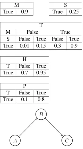
Figure 2.1 presents a Bayesian network for a traveling activity. This example shows a discrete Bayesian network with a domain of ﬁve Boolean variables, which include and are represented as follows:

(32)

A B

C

D E

Figure 2.1: A simple BN for modeling a traveling activity

1) S – the event that it is summer time; 2) M – the event that the person has money; 3) T – the event that the person is going to travel; 4) H – the event that the person is happy; and

5) P – the even that the person is going to meet new people.

Instead of enumerating the probability distributions of the five domain variables used in figure 2.1 (25 possible combinations), We define the joint probability distribution of this Bayesian network as indicated:

P(S, M, T, H, P) =P(S)×P(M)×P(T |S, M)×P(H |T)×P(P |T)

2.2 THE NOTION OF D-SEPARATION

In a Bayesian network, there are three basic connections among variables as follows [48]:

1. Serial connections(also calledpipelined influences): in a serial connection (shown in figure 2.2), changes in the certainty of A will affect the certainty B, which in turn will affect the uncertainty of C. Therefore this shows information may flow from node A through B to C, unless there is evidence about B (B is known, or B isinstantiated).

(33)

Table 2.1: Conditional probability tables for a simple BN for modeling a traveling activity

M S

True 0.9 True 0.25

T

M False True

S False True False True True 0.01 0.15 0.3 0.9 H T False True True 0.7 0.95 P T False True True 0.1 0.8 A B C

Figure 2.2: An example of a serial Connection B

A C

Figure 2.3: An example of a diverging connection

2. Diverging connections: in a diverging connection (shown in ﬁgure 2.3), changes in the certainty of A will affect the certainty B, which in turn will affect the uncertainty of C. Therefore this shows information may ﬂow from node A through B to C, unless there is evidence about B.

3. Converging connections (a.k.a. v-structure): in a converging connection (shown in ﬁgure 2.4), changes in the certainty of A cannot affect the certainty C through B, and

(34)

B

A C

Figure 2.4: An example of a converging connection

vice versa. Therefore this shows information cannot ﬂow between A and C through B, unless there is evidence about B.

The previously discussed three types of connections in a casual network are used in the deﬁnition ofd-separation[48]:

Deﬁnition 2.2. (d-separation)

Two distinct variables A and B in a causal network are d-separated ("d" for "directed graph") if for all paths between A and B, there is an intermediate variable V (distinct from A and B) such that either

• the connection is serial or diverging and V is instantiated, or

• the connection is converging, and neither V nor any of V’s descendants have received evidence.

2.3 STRUCTURE LEARNING INBAYESIANNETWORKS

There are three main approaches to learn the structure of Bayesian networks: constraint-based,score-based, orhybridalgorithms.

(I) Constraint-based algorithms count on conditional independence tests to determine the DAG of the learned Bayesian network. The Inductive Causation (IC) algo-rithm [64] was the ﬁrst constraint-based algoalgo-rithm, which introduced a framework for learning the structure of causal models. IC’s framework consists of three steps as follows:

(35)

(i) Find the skeleton (all pairs of dependent variables) (ii) Remove indirect dependencies (by deﬁning colliders)

(iii) Complete orienting the remaining undirected edges if any (avoiding cycles). All constraint-based algorithms, such as the PC algorithm [60, 61] and NPC algo-rithm [62], follow the theoretical framework introduced by the IC algoalgo-rithm.

(II) Score-based algorithms, such as AIC [1], BDe [56], K2 [21], and BIC algorithm [27], assign a score for each Bayesian network structure (this score indicates how well the Bayesian network structure ﬁts the data) and then perform a (usually greedy) search algorithm to select the structure with the highest score.

(III) Hybrid algorithms, such as CB [59] and EGS algorithm [22], rely on the idea of using both based algorithms and score-based algorithms. The use of constraint-based algorithms will reduce the search space (i.e., it will reduce the number of candidate DAGs). Thenceforth, score-based algorithms can be used to select the optimal DAG.

We will focus on the PC algorithm since it is an integral part of this paper. The PC al-gorithm(named after the authors, the ﬁrst letter of their ﬁrst names,Peter Spirtes andClark Glymour) is a constraint-based algorithm for learning the structure of a Bayesian network from data. The PC algorithm follows the theoretical framework of the IC algorithm to de-termine the structure of causal models [57, 53]. According to [61], the process performed by the PC algorithm to learn the structure of Bayesian networks can be summarized as follows:

(i) For every pair of variables, perform statistical tests for conditional independence. (ii) Determine the skeleton (undirected graph) of the learned structure by adding a link

(36)

(iii) Identify colliders (v-structures) of the learned structure (A→B←C). (iv) Identify derived directions.

(v) Randomly, complete orienting the remaining undirected edges without creating a new collider or a cycle.

For the implementation of this paper, we usedthe Hugin PC algorithm(byHuginT M De-cision Engine[49, 38]), "which is a variant of the original PC algorithm due to [61]" [29].

2.4 PRIOR TO POSTERIORUPDATING

Bayes’ theorem is a simple mathematical formula that inverts conditional probabilities (i.e., given the conditional probability of eventBgiven eventA, how to calculate the conditional probability of eventAgiven eventB). The statement of Bayes’ theorem is: For two events AandB,

P(A|B) = P(B |A)P(A)

P(B) ,

where

(i) P(A|B)is the conditional probability of eventAgiven eventB(called the posterior probability),

(ii) P(B | A)is the conditional probability of event B given eventA (called the likeli-hood),

(iii) P(A)is the marginal probability of eventA(called the prior probability), and (iv) P(B)is the marginal probability of eventB(P(B)>0) [45].

Unlike classical statistics, Bayesian statistics treats parameters as random variables whereas data is treated as ﬁxed. For Example, letθ be a parameter, andD be a dataset, then Bayes’ theorem can be expressed mathematically as follows:

P(θ |D) = P(D|θ)P(θ)

(37)

In equation 2.3, P(θ | D) is the posterior distribution, which is the ultimate goal for Bayesian statistics since it measures the uncertainty about the parametersθafter seeing the datasetD. P(D|θ) is thelikelihood, which describes how likely the dataset D is if the truth is parameterθ. P(θ)is theprior distribution, which is a marginal probability of our belief before seeing data.P(D)is themarginal probabilityofD, which is a normalization constant to ensures that the sum of the posterior distribution sums to 1 over all values of parameterθ[36]. Thus, sinceP(D)is constant, we can write Bayes’ theorem in one of the most useful form in Bayesian update and inference as follows:

P(θ |D)∝P(D|θ)×P(θ) (2.4)

P osterior∝Likelihood×P rior (2.5)

In Bayesian analysis, the results of the experiment could be used to update the belief about the parameterθ. In simple cases, we can compute the posterior distribution for the parameterθ by multiplying the prior distribution and the likelihood function as shown in equation 2.5. However, it is convenient mathematically for the prior and the likelihood to be conjugate. A prior distribution is a conjugate prior for the likelihood function if the posterior distribution belongs to the same distribution as the prior [54]. For example, the beta distribution is a conjugate prior for the binomial distribution (as a likelihood function) because the posterior distribution obtained by multiplying the prior and the likelihood be-longs to the same distribution as the prior (thus, both the prior and the posterior have beta distributions).

Let’s consider the effect of different priors on the posterior distribution. A completely uninformative prior is the beta distribution with parametersα= 1andβ= 1. The posterior distribution in this case is equivalent to the likelihood function since we have a completely uninformative prior. More informative priors will have a greater inﬂuence on the poste-rior distribution for a given sample size. On the other hand, larger sample sizes will give the likelihood function more inﬂuence on the posterior distribution for a given prior dis-tribution. In practice, this means that we can obtain a precise estimate of the posterior

(38)

distribution using smaller sample sizes when we use more informative priors. Similarly, we may need larger sample sizes when we use a weak or uninformative prior.

P(θ |D)∝Beta(α, β)×Binomial(n, θ) (2.6)

P(θ |D)∝Beta(y+α, n−y+β) (2.7)

Equation 2.7 is the formula that we are going to use in this paper for prior to posterior update. Starting with a prior distributionBeta(α, β), we add the count of successes,y, and the count of failures,n−y, from the datasetD (wheren is total number of entries inD) toαandβ, respectively. Thus,Beta(y+α, n−y+β)is the posterior distribution. For a theoretical justiﬁcation of the use of the beta distribution to model parameter uncertainty, see [45].

2.5 LINK STRENGTHS IN BAYESIANNETWORKS

The concept of link strength in Bayesian networks was introduced ﬁrst by Boerlage in 1992 [18]. In his thesis, Boerlage introduced the concepts of both connection strength and link strength in a binary Bayesian network model. Connection strength for any two variables A andB in a Bayesian network model B1 is deﬁned as measuring the strength

between these two variables by testing all possible paths between them in B1, whereas link strengthis defined as measuring the strength these two random variables taking into account only the direct edge A−B [18]. Methods for link strengths measurements are not studied sufficiently. Imme Ebert-Uphoff in her 2009 paper [24] presented a tutorial on how to measure connection strengths and link strengths in discrete Bayesian networks. Ebert-Uphoff concluded that there is a limited literature on link strengths, and there is more need to apply and use link strengths measures in structure learning and other purposes [24]. However, to the authors’ best knowledge, there are no more recent publications that address link strengths measurements in discrete Bayesian networks. In this paper, we define a novel and not computationally expensive link strengths measure in discrete Bayesian networks.

(39)

2.6 ADVERSARIAL MACHINELEARNING

Adversarial machine learning is the research field that studies the design of efficient ma-chine learning algorithms in adversarial environments [28]. Attacks against mama-chine learn-ing systems have been organized by [11, 10, 28] accordlearn-ing to three features: Influence, Security Violation, and Specificity. First, influence of the attacks on machine learning models can be either causative or exploratory. Causative attacks aim to corrupt the training data whereas exploratory attacks aim to corrupt the classifier at test time. Second, security violation of machine learning models can be a violation of integrity, availability, or privacy. An integrity violation is an attack that aims to misclassify false positives with the goal of gaining unauthorized access to the system. An availability violation is an attack that aims to misclassify both false positives and false negatives and leads to denial of service. A privacy violation is an attack in which an adversary is able to reap confidential information from a machine learning model. Third, specificity of the attacks against machine learning models can be either targeted, or indiscriminate. Targeted attacks aim to corrupt machine learning models to misclassify a particular class of false positives whereas indiscriminate attacks have the goal of misclassifying all false positives.

Evasion attacks [63, 13, 26, 33, 31] and Data poisoning attacks [16, 41, 40, 2] are two of the most common attacks on machine learning systems [28]. Evasion attacks are exploratory attacks at the testing phase. In an evasion attack, an adversary attempts to pollute the data for testing the machine learning classifier; thus causing the classifier to misclassify adversarial examples as legitimate ones. Data poisoning attacks are causative attacks, in which an adversary attempts to corrupt the machine learning classifier itself by contaminating the data on training phase.

In this dissertation, we study the resilience of two commonly used Bayesian network al-gorithms, namely the PC algorithm and the LCD algorithm, against data poisoning attacks. Since no study has been performed on evaluating the vulnerabilities of these algorithms against poisoning attacks, we will just explore the line of data poisoning research on

(40)

dif-ferent machine learning ﬁelds.

There has been a long line of work on poisoning attacks of support vector machines (SVMs) [16, 66, 67, 47, 42, 19, 32]. In Neural Networks (NNs), there has been a recent study of data poisoning attacks in which the authors investigated the process of data gener-ation poisoning and proposed two poisoning methods, including a direct gradient method and a generative method [69].

2.7 DEFENSES AND COUNTERMEASURES FORDATA POISONING ATTACKS

In this section, we will give a brief overview of adversarial machine learning research; focusing on data poisoning. Recent surveys on adversarial machine learning can be found in [10, 25, 35].

2.7.1 DATAPOISONINGATTACKS

As machine learning algorithms have been widely used in security-critical settings such as spam filtering and intrusion detection, adversarial machine learning has become an emerging field of study. Attacks against machine learning systems have been organized by [11, 10, 28] according to three features: Influence, Security Violation, and Specificity. Influence of the attacks on machine learning models can be either causative or exploratory. Causative attacks aim to corrupt the training data whereas exploratory attacks aim to cor-rupt the classifier at test time. Security violation of machine learning models can be a violation of integrity, availability, or privacy. Specificity of the attacks can be either tar-geted or indiscriminate. Tartar-geted attacks aim to corrupt machine learning models to mis-classify a particular class of false positives whereas indiscriminate attacks have the goal of misclassifying all false positives.

Evasion attacks and Data poisoning attacks are two of the most common attacks on machine learning systems [28]. Evasion attacks [26, 33, 31] are exploratory attacks at the testing phase. In an evasion attack, an adversary attempts to pollute the data for testing the

(41)

machine learning classifier; thus causing the classifier to misclassify adversarial examples as legitimate ones. Data poisoning attacks [40, 2, 16, 42, 32, 69] are causative attacks, in which adversaries attempt to corrupt the machine learning classifier itself by contaminating the data in the training phase.

Data poisoning attacks have been studied extensively during the last decade [43, 6, 16, 42, 32, 15, 14, 17, 12, 69]. However, attacks against Bayesian network algorithm have not been studied. In our previous work, we were addressed data poisoning attacks against Bayesian network algorithms [8, 9, 6]. We studied how an adversary could corrupt the Bayesian network structure learning algorithms by inserting contaminated data into the training phase. We showed how our novel measure of strengths of links for Bayesian net-works [9] can be used to do a security analysis of attacks against Bayesian network struc-ture learning algorithms. However, our approach did not consider long-duration attacks.

2.7.2 DEFENSES ANDCOUNTERMEASURES

Data sanitization is a best practice for security optimization in the adversarial machine learning context [20]. It is often impossible to validate every data source. In the event of a poisoning attack, data sanitization adds a layer of protection for training data by removing contaminated samples from the targeted training data set prior to training a classifier. Reject on Negative Impact is one of the widely used method for data sanitization [10, 20, 35]. Reject on Negative Impact defense assesses the impact of new training sample additions, opting to remover or discard samples that yield significant, negative effects on the observed learning outcomes or classification accuracy [10, 20]. The base training set is used to train a classifier, after which, the new training instance is added and a second classifier is trained [10]. In this approach, classification performance is evaluated by comparing error rates (accuracy) between the original and the new, retrained classifier resulting from new sample integration [35]. As such, if new classification errors are substantially higher

(42)

compared to the original or baseline classiﬁer, it is assumed that the newly added samples are malicious or contaminated and are therefore removed in order to maximize and protect classiﬁcation accuracy [10].

(43)

C

HAPTER

3 O

VERVIEW OF THE

P

ROPOSED

S

YSTEM

3.1 OVERVIEW OF ADVERSARIALATTACKS AGAINSTBAYESIANNETWORK

MODELS

Data integrity is a key requirement for correct machine learning applications, such as Bayesian network structure learning algorithms. In this research, we study how an ad-versary could corrupt the PC structure learning algorithm. An attacker may attempt to corrupt the machine learning model by poisoning the input dataset with the ultimate goal of inﬂuencing the output model. In this research, we propose a threat model to investigate both attacks that aim to arbitrarily invalidate the learning outcome and attacks that aim to achieve a speciﬁc goal. We use this threat model to study the resilience of Bayesian network algorithms, namely the PC algorithm, against data poisoning attacks.

Like all security problems, the problem of adversarial attacks against Bayesian net-works is to design a security prevention and detection model against these attacks. Our ongoing work is about developing prevention methods against these deﬁned attacks.

3.2 THREATMODEL FOR DATAPOISONINGATTACKS AGAINST THE PC ALGORITHM

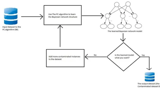
In this section, we present the general framework of how attackers can use exploratory at-tacks to corrupt the learned Bayesian model by the PC algorithm. The attacker ﬁrst uses the PC algorithm to learn the structure of the Bayesian network model. If the learned structure is what the adversarial opponent wants, then the “poisoned" datasetDB2 is

(44)

pro-duced. Otherwise, the user adds contaminated cases to the learning dataset and relearn the Bayesian model using the PC algorithm until the desired model is obtained. This process is illustrated in Figure 3.1.

Figure 3.1: Overview of how data poisoning attacks against Bayesian network structure learning algorithms work.

In this dissertation, we study the resilience of two of the most commonly used Bayesian network algorithms, namely the PC algorithm and the LCD algorithm, against data poison-ing attacks. To the authors’ best knowledge, no study has been performed on evaluatpoison-ing the vulnerabilities of Bayesian network structure learning algorithms against poisoning attacks. We present the two subclasses of data poisoning attacks against the Bayesian network al-gorithms: 1) Model invalidation attacks and 2) Targeted change attacks.

(45)

C

HAPTER

4 L

INK

S

TRENGTHS FROM

D

ATA IN

D

ISCRETE

B

AYESIAN

N

ETWORKS

4.1 INTRODUCTION

We introduce a novel link strengths measure between two random variables in a discrete Bayesian network model (denoted as L_S). It is essential to not only study the existence of a link in a causal model but also define a reliable link strengths measure that is useful in Bayesian reasoning [18, 24]. The new defined link strengths measure assigns a number to every link in a Bayesian network model. This number represents the lowest confidence of all possible combinations of assignments of posterior distributions. The defined link strengths measure will be used to rank edges from the most to the least believable edge, rank edges from the weakest to the strongest edge, and justify a plausible process in any causal model.

4.2 DEFINITION OF THEPROPOSED LINK STRENGTHSMEASURE (L_S)

In this section, we present the deﬁnition of our new link strength measure (we named it L_S). Our novel approach is as follows:

Deﬁnition 4.1. The link strengths measure (L_S) is deﬁned as

L_S(V ariable1 →V ariable2) = min y∈Y(pdf(

y+α

α+n+β);α, β, y, n) (4.1) whereY ={n11, n12, . . . , n1j, n21, n22, . . . , n2j, . . . , ni1, ni2, . . . , nij},pdf is the

(46)

4.3 EXPLANATION

Given a discrete dataset DB1 and a Bayesian network structure B1 learned by the PC

algorithm usingDB1, for every linkV ariable1 → V ariable2 inB1, build a contingency

table [39] for the two discrete variables V ariable1 and V ariable2 with i and j states,

respectively (as shown in table 4.1).

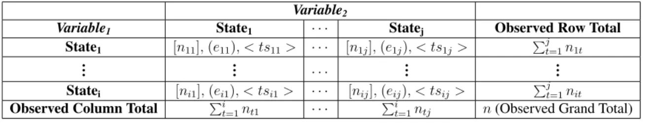
Table 4.1: A contingency table for two discrete variablesV ariable1 andV ariable2withi

andj states, respectively.

Variable2

Variable1 State1 · · · Statej Observed Row Total State1 [n11],(e11), < ts11> · · · [n1j],(e1j), < ts1j > ∑jt=1n1t .. . ... · · · ... ... Statei [ni1],(ei1), < tsi1> · · · [nij],(eij), < tsij> ∑j t=1nit Observed Column Total ∑it=1nt1 · · ·

∑i

t=1ntj n(Observed Grand Total)

The above contingency table (Table 4.1) is structured as follows: 1. [nij]is the cell’s observed counts obtained from datasetDB1,

2. (eij) is the cell’s expected counts, calculated as follows:

Observed Row Total×Observed Column Total Observed Grand Total (denoted as n) 3. < tsij >is the cell’s chi-square test statistic, calculated as follows:

(nij −eij)2

eij

To measure the strength of links of a causal model, we perform the following two steps: (1) We compute the posterior distributions for each linkV ariable1 → V ariable2 as

fol-lows:

(47)

whereV ariable2 |V ariable1is all possible combinations of discrete states ofV ariable2

andV ariable1, and then

(2) We use our link strengths measure as presented in equation 4.1.

Note that _α₊y+_nα₊_β in equation 4.1 is obtained by simply substitutingαwithy+αandβwith n−y+β in _α₊α_β.

4.4 INTERPRETATION

For any two random variables in a causal model (V ariable1 with i states and V ariable2

withj states), there arei×j combinations of assignments of posterior distributions. For every posterior distribution, we have a prior distribution that is a conjugate prior for the likelihood function. For instance, a posterior distribution in the formBeta(y+α, n−y+

β)has a Beta-distributed prior, Beta(α, β), which is a conjugate prior for the likelihood function,Binomial(n, θ). Considering alli×j posterior distributions for the two random V ariable1 andV ariable2, we can measure the uncertainty of that link by measuring how

peaked the posterior distributions (Beta distributions in our experiments) are; thus, we can identify the link strength based on the uncertainty level. The more peaked the posterior distribution is, the more certainty we have about the posterior distribution probability. The peak of a beta distribution,Beta(α′, β′), is reached at its mean,_α_′α₊′_β_′. Thus, the peak of the posterior distribution is reached at _n₋y−_y₊α_β. In the deﬁned link strengths measure, we deﬁne the link strength for any link between two random variables in a causal model as the value of the smallest peak. This point is the point at which the model has seen the fewest number of cases; thus, it is the most critical point through which this link can be manipulated.

4.5 PRACTICAL USAGES

We use this measure to identify weak edges (i.e., low values ofL_S). These edges are the easiest to remove from a given causal model. We also use theL_Svalue to identify location

(48)

Table 4.2: Posterior distributions for the Chest Clinic Network.

Link

Posterior Distributions (Beta Distributions)

P(T

|

A)

Beta(10,99) Beta(106,9789) Beta(99,10) Beta(9789,106)

P(L

|

S)

Beta(481,4510) Beta(47,4966) Beta(4510,481) Beta(4966,47)

P(B

|

S)

Beta(3019,1972) Beta(1514,3899) Beta(1972,3019) Beta(3899,1514)

P(E

|

T)

Beta(115,1) Beta(523,9365) Beta(1,115) Beta(9365,523)

P(E

|

L)

Beta(527,1) Beta(111,9365) Beta(1,527) Beta(9365,111)

P(D

|

B)

Beta(3638,895) Beta(725,4746) Beta(895,3638) Beta(4746,725)

P(D

|

E)

Beta(520,118) Beta(3843,5523) Beta(118,520) Beta(5523,3843)

P(X

|

E)

Beta(624,14) Beta(454,8912) Beta(14,624) Beta(8912,454)

for new edges to be added. We claim that the highestL_S value, the most believable the new edge is.

4.6 EXPERIMENTALRESULTS

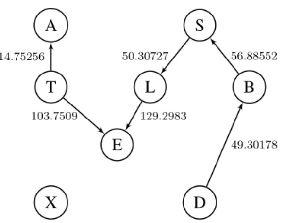
In this section, we will evaluate the proposed link strength measure (L_S) on the original Chest Clinic Network. Given the Chest Clinic network model as shown in Figure 1.3 and the datasetDB1, we followed thetwo stepspresented in section 4.

Table 4.2 contains the posterior distributions (Beta Distributions) calculated in step 1 as follows:

Figure 4.1 shows the ﬁnal link strength evaluation (L_S) which is calculated instep 2 as follows:

We observe that the edgeT →Ais the weakest edge in Chest Clinic network with the score14.75256. Also, we can see that the edgeE →Dis the second weakest edge with the score25.73502and so on. The strongest edge in Chest Clinic network is the edgeL →E with the score129.2983.

4.7 COMPARISON WITHPREVIOUS LINK STRENGTH MEASURES

In this section, we will compare our link strength measure(L_S)with Mutual Information link strengths measure. Shannon in [58] introduced the concept of Mutual Information

(49)

A S T L B E X D 14.75256 50.30727 56.88552 129.2983 103.7509 70.69412 25.73502 49.30178

Figure 4.1: Results ofL_S on the Chest Clinic Network.

(M I) in the context of communication theory and Pearl in [52] proposed its expanded use to measure connection strength in Bayesian Networks; it is deﬁned as:

M I(X, Y) =∑ x,y

P(x, y)log2(

P(x, y)

P(x)P(y)) (4.2)

M Imeasures the how edge in a causal model are related to each others by (1) detecting any sort of relationship and (2) employing straightforward interpretation of the amount of data shared between the datasets (3) while remaining insensitive to dataset size, as characteristic of p-value testing [55]. This simplified M I calculation reflects and measures connection strength between X and Y based on the degree or strength of influence the state of X affects the state of Y through the comparison of U(Y) and U(Y|X). Put another way, the MI formula seeks to determine the amount of uncertainty in Y that can be reduced by knowledge of state of X if nothing else is known [24]. Therefore, the M I between two datasets (X and Y) is typically estimated from statistical analysis of the (x, y)pairs between the two datasets [55].

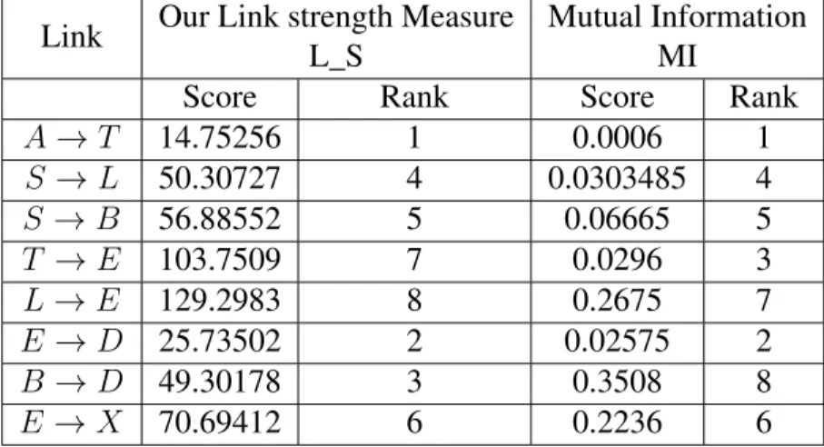
The following table (Table 4.3) presents the results of using our link strength (L_S) and MI link strength to compute strengths of links of the Chest Clink Network. Note that, we

(50)

rank the edge in the columnrankfrom the weakest to the strongest edge. For more technical details about how to use MI link strength measure, we refer the reader to Appendix C. Table 4.3: Using L_S and MI to compute link strength of the original Chest Clinic Network

Link Our Link strength Measure L_S

Mutual Information MI

Score Rank Score Rank

A→T 14.75256 1 0.0006 1 S →L 50.30727 4 0.0303485 4 S→B 56.88552 5 0.06665 5 T →E 103.7509 7 0.0296 3 L→E 129.2983 8 0.2675 7 E →D 25.73502 2 0.02575 2 B →D 49.30178 3 0.3508 8 E →X 70.69412 6 0.2236 6

Both link strengths measures agree on the fact that the edge A → T is the weakest link in the Chest Clinic Network. However, our link strength measure functions better since it is able to identify the deterministic edges. That is, deterministic edges T → E andL → E are hard edges to break. In addition, MI measure computes the link strength measure using the conditional probability tables whereas our link strength measure uses a given dataset to compute the strengths of links, which makes our link strength efﬁcient for security application as it is sensitive to changes in data.

(51)

C

HAPTER

5 M

ODEL

I

NVALIDATION

A

TTACKS

5.1 OVERVIEW OF MODELINVALIDATIONATTACKS

A model invalidation attackagainst the PC algorithm is a malicious active attack in which adversarial opponents try to corrupt the original model in any way. We demonstrate ad-versarial attacks to decrease the validation status of the model using the least number of changes.

In such an event, adversaries create some formal disturbance in the model. For example, they will try to add imprecise or incorrect data to change the model validation status so that the model is rendered invalid. We distinguish between two ways to invalidate Bayesian network models:

1) Attacks based on the notion of d-separation and 2) Attacks based on marginal independence tests.

In what follows, we present an item list and short description for all the algorithms that are going to be presented in this chapter of the dissertation:

Algorithm Description

Algorithm 1 Creating a New Converging Connection Algorithm 2 Breaking an Existing Converging Connection

Algorithm 3 Edge Deleting

Algorithm 4 Removing a Weak Edge

Algorithm 5 Edge adding

(52)

5.2 MODELINVALIDATION ATTACKS BASED ON THE NOTION OF D-SEPARATION

Based on the deﬁnition of d-separation, adversaries may attempt to introduce a new link in any triple(A−B−C)in the BN model. This newly inserted link(A−C)will introduce a v-structure in the Bayesian model, thus change the independence relations.

Theorem 5.1. Let B1 and B2 be two Markov equivalent BNs, and let < A, B, C > be

a path in B1. If a new link is added to B1 creating B1′, then B′1 and B2 are not Markov equivalent.

B

A C

(a) Adding the dashed link to the serial connection.

B

A C

(b) Adding one of the dashed links to the diverging connection.

B

A C

(c) Adding one of the dashed links and shielding colliderB. Figure 5.1: Three cases for the proof of Theorem 5.1.

Proof Sketch. Adding a new edge to the path< A, B, C >in Bayesian network modelB1

affects the Markov equivalence class ofB1(two Bayesian networks areMarkov equivalent

if and only if they have the same skeleton and the same v-structures (unshielded collid-ers) [3]). Any sound learning algorithm will try to avoid the occurrence of a cycle; thus, in