Evaluating German Business Cycle Forecasts Under an Asymmetric Loss Function

(1)

Department Economics and Politics

Evaluating German Business Cycle

Forecasts Under an Asymmetric Loss

Function

Jörg Döpke

Ulrich Fritsche

Boriss Siliverstovs

DEP Discussion Papers

Macroeconomics and Finance Series

5/2009

(2)

Under an Asymmetric Loss Function

by

Jörg Döpke (University of Applied Sciences Merseburg)1

Ulrich Fritsche (Hamburg University and DIW Berlin)2

Boriss Siliverstovs (KOF, ETH Zurich)3

December 2008

Abstract

Based on annual data for growth and inflation forecasts for Germany covering the time span from 1970 to 2007 and up to 17 different forecasts per year, we test for a possible asymmetry of the forecasters' loss function and estimate the degree of asymmetry for each forecasting institution using the approach of Elliot et al. (2005). Furthermore, we test for the rationality of the forecasts under the assumption of a possibly asymmetric loss function and for the features of an optimal forecast under the assumption of a generalized loss function. We find only limited evidence for the existence of an asymmetric loss functions of German forecasters. As regards the rationality of the forecasts the results depend on the underlying assumption of the test. The rationality of inflation forecasts is more doubtful than those of growth forecasts.

Keywords: Business cycle forecast evaluation, asymmetric loss function, and rational expectations.

JEL-Classification: C53, E42

1_{The authors thank Gerit Vogt, participants at the 3}rd_{Dresden Workshop on Business Cycles and Macroeconomics 2008,}

and at the 9th_{Macroeconometric Workshop in Halle for helpful comments on a previous draft of this paper. Corresponding}

author: Jörg Döpke, University of Applied Sciences Merseburg, D-06217 Merseburg/Germany. Phone: +49-(0)3461 462441. E-mail: [email protected].

2_{Ulrich Fritsche, Hamburg University, Faculty Economics and Social Sciences and German Institute of Economic}

Research, von-Melle-Park 9, D-20146 Hamburg/Germany, Phone: +49-(0)40 42838 2098, E-Mail:

[email protected] .

3_{Boriss Siliverstovs, KOF Swiss Economic Institute, Eidgenössische Technische Hochschule Zürich (ETHZ) (Federal}

(3)

1. Introduction

The assumption that economic agents behave rationally when they form their expectations is a central assumption in economics and finance. Consequently, a large body of literature has

investigated the accuracy and rationality of forecasts, including several studies regarding German business cycle forecasts (see, e.g., Fildes and Stekler, 2002, for a survey and Döpke and Fritsche, 2006 for an overview of related papers for German data). Virtually all these studies, however, regardless of whether made explicitly or implicitly, analyse the issue under the assumption of a symmetric loss function; i.e., the notion that over- and underestimations are equally costly to the respective forecaster. While this assumption has been more or less undisputed for a long period of time, it may be criticised for very good economic reasons.

Consider possible customers of business cycle forecasters: For example, for a single firm, there is

a priori absolutely no reason why the costs of underpredicting demand in terms of a loss of sales or

reputation should be exactly equal to the costs of overpredicting demand in terms of additional cost and storage (Elliot et al., 2005, 2008). On a macroeconomic level, it is very likely that e.g. central banks have asymmetric preferences regarding inflation, perhaps in the direction of more caution against inflation acceleration. Alan Blinder summarises his experience as a central bank officer, claiming that a central bank “take (s) far more political heat it tightens preemptively to avoid higher inflation than it eases preemptively to avoid higher unemployment” (Blinder, 1998). Furthermore, while a overestimation of a budget deficit may foster the career of a finance minister, an

underestimation may end it. Or, as famous German economist and politician Ludwig Erhardt put it: ”If it gets better than expected, even the false prophet will be forgiven” (quoted according to, e.g., Miersch, 2008). Furthermore, international or supranational institutions like IMF, World Bank, or

(4)

the European Commission face agency problems regarding their relationships with clients or

member states – which, in turn, could justify asymmetric loss functions (Artis and Marcellino: Elliott et al., 2005; Christodoulakis and Mamatzakis 2008, 2009). An additional line of argumentation, which may point to the possibility of an asymmetric loss, is the political economy of business cycle forecasts (see Döpke 2000 for related arguments). In this view, individual forecasters represent competing political points of view and use the forecasts as instruments to achieve their political goals. Hence, under- and overestimations of growth and inflation are likely to be unequally costly in the eyes of the forecaster, since they give different incentives for good or bad policies. All in all, a certain scepticism regarding the symmetry assumption is therefore well justified. We will therefore analyse signs for asymmetric loss functions for those institutions publishing regular forecasts for the German economy.

Consequently, several approaches have been developed to incorporate more general loss function into forecasting evaluations. Based on influential work by Chistofferson and Diebold (1997),

Granger (1999), and Batchelor and Peel (1998), among others, Elliott et al. (2005, 2008) have proposed to estimate the degree of asymmetry of the loss function and to test for a significant degree of asymmetry. Moreover, Patton and Timmerman (2007) analysed the properties of an optimal forecast under a generalised loss function and discussed how to test for these properties. We make use of these approaches to re-evaluate the issue of rationality of the German business cycle forecasts; namely growth and inflation forecasts covering the time span from 1970 to 2007 and up to 17

different forecasts.

(5)

respect: some forecasters seem to have incentives for pessimistic forecasts; others, for too-optimistic forecasts. Over and above this, the results appear to be not fully robust against the choice of the instruments warranted to estimate the loss function with an Instrumental Variable (IV) estimator.

Furthermore, we check whether the usual results concerning the rationality of the forecasts still hold, when the assumption regarding the loss function is relaxed. In a nutshell, we find that neither a specifically asymmetric loss function nor the assumption of a generalized loss function alter the findings obtained under a symmetric loss function by very much, though the results of the test proposed by Elliot et al. (2005) give some contrary results for inflation forecasts.

The remainder of the paper is organised as follows: Section 2 describes the data and presents some general statistics on forecast accuracy. Section 3 describes the econometric method proposed by Elliot et al. (2005) to back out the parameter of asymmetry of a loss function and statistical testing for the existence of asymmetry and discusses the results for the data set at hand. Section 4 tests for the rationality of the forecasts under different assumptions: a symmetric loss function, an specific asymmetric loss function, and a generalised loss function. The final section summarises and concludes.

2. Data and descriptive statistics

(6)

forecasts regarding the German economy. Details on the data set under investigation can be found in Döpke and Fritsche (2006). For all institutions, we have collected the growth and inflation forecasts. The growth forecast is the predicted growth rate of real GNP (for the time span 1983 to 1989) and of real GDP (for all other years). In case of published interval forecasts the average is used. The

numbers refer to West Germany up to 1992, and to the whole of Germany from 1993 to present. As a measure of the inflation forecast we use the predicted change of the deflator of private

consumption when this figure was available. In some cases, however, no explicit reference was given whether a mentioned inflation forecast referred to the consumption deflator or to the CPI/ HICP. In such cases we assume that no distinction between the figures was intended by the

forecaster and used the available inflation forecast. As regards the actual outcome, it is possible to refer to the last available revised data or to the first published ("real-time") data. As it is common in the analysis of business cycle forecasts, we make use of the latter type of numbers i.e. we compare the forecasts made at the end of a certain year "x" or at the beginning of the following year "x+1" with the first published figure for the year "x+1”.

To give a first impression of some forecast properties and the forecast errors, Table 1 presents a couple of standard measures of forecast accuracy for each institution separately. In particular, we calculate the following statistics:4

i. The mean error

∑

= + = T t t e T ME 1 1 1

, where et+1= yt+1− yˆt+1 is the forecast error in each period,

defined as actual (in t+1) minus predicted (in t for period t+1) value of the variable y. Thus, a positive (negative) value of the mean error corresponds to an under (over-) estimation of the growth rate. Subscript t is the time index.

(7)

∑

₌

t

T 1

iii. The root mean squared error

∑

= + = T t t e T RMSE 1 2 1 1 .

iv. A version of Theil's coefficient, which compares the RMSE of the forecast under

investigation with the RMSE of a “naive” forecast. In our case, the naïve forecast is given by a “no change” forecast in terms of growth rates, i.e. for the following year the same growth or inflation rate than in the previous year is predicted. A value greater than one for the coefficient indicates that the forecast is worse than the naïve forecast.

v. The first order autocorrelation coefficient of the forecast errors.

 Insert Table 1 here 

Turning to our results, the findings in Table 1 confirm the findings of a lot of previous studies. To begin with, the mean error of the growth forecasts is negative in all but one case suggesting on average a slight tendency of the forecasters to be too optimistic. The absolute and root mean squared errors indicate the magnitude of the forecast errors, which is, as has often been documented by various authors (see Döpke and Fritsche 2006 and the literature cited therein), substantial and exceeds by far the expectations on forecast accuracy by public opinion. As far as the growth

forecasts are concerned, however, Theil’s coefficient suggests that the forecasts still contain valuable information when compared to a “no change”-forecast. By contrast, this does not hold for the

(8)

fact that inflation is typically a quite persistent process – empirically even often indistinguishable from a random walk process – whose “optimal” forecast is often found to be close to or identical with the last observation. This is further supported by the first order correlation coefficient reported in the last column of Table 1: while the respective numbers for the growth forecasts are usually small with alternating signs, the autocorrelation of the inflation forecast errors is consistently positive and frequently quite large.

3. Estimating loss function asymmetry parameters and testing for asymmetry

The analysis by Elliot et al. (2005) starts from the general loss function:

Lp ,,=[1−2⋅1yt1− yt10∣yt1− yt1∣p] (1)

In this loss function the parameter p represents the underlying assumption of the subsequent analysis. In particular, p=1 stand for a linear-linear (lin-lin) loss function, while in case of p=2 the calculations are based on a quadratic-quadratic (quad-quad) loss function. Furthermore, the loss function consists of a parameter  . It represents the degree of asymmetry of the loss function. In particular, =0.5 yields a symmetric loss function, while 0.5 represents the case of forecasters' incentives to issue optimistic forecasts. Finally, 0.5 stands for the case of too-pessimistic forecasts. Thus, a particular set of parameters leads to well-known loss function. For example L1,1/2,=yt1− yt1

2

yields a symmetric quadratic loss function (Elliot et al. 2005: 1110). The key problem addressed by Elliot et al. (2005) is, of course, that the value of this

(9)

Elliot et al. (2005) establish conditions for optimality of forecasts, which, in turn, deliver the moment condition for the IV estimator. By observing the sequence of forecasts, the authors propose a GMM estimator that yields the following expression to estimate the asymmetry parameter of the loss function out of the moment condition:

 _T=

[

1 T

∑

t= T−1 _t

_∣

y_t_₁− y_t_₁

_∣

p0−1

]

'  S−1

[

1 T

∑

t= T−1 _t1y_t_₁− y_t_₁0∣y_t_₁− y_t_₁∣p0−1

]

[

1 T

∑

t= T−1 _t

_∣

y_t_₁− y_t_1∣p0−1

]

'_S−1

[

1 T

∑

t= T−1 _t∣y_t_₁− y_t_₁∣p0−1

]

(2) with . S= 1 T  '1yt1− yt10−t 2 ∣yt1− yt1∣ 2p0−2

as a weighting matrix. Since S depends on _T , estimation has to be performed iteratively, assuming S = I in the first round since the identity matrix is a consistent starting point and using v_t as instrument(s). Hence, the estimation is based on considerations that have led to the GMM estimator proposed by Hansen (see Hansen and West, 2002, for a survey and a discussion of its relation to macroeconomic applications). Elliot et al. (2005) show that the estimator of _T is asymptotically normal and, hence, renders it possible to test for the hypothesis =0.5 i.e. for loss function symmetry.

For the proposed GMM estimator appropriate instruments are warranted. Following Elliot et al. (2005: 461), our instruments are: i) a constant; ii) a constant and a lagged forecast error; iii) a

constant and the lagged variable to be predicted (i.e. the growth and inflation rate, respectively); and iv) a constant, the lagged forecast error, and the lagged variable to be predicted. The estimation

(10)

results for the data set under investigation are given in Table 2.

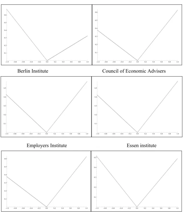
Αs regards the growth forecasts and the calculations based on the assumption of a lin-lin loss function the findings revealed in Table 2 suggest only very limited evidence for asymmetric loss functions. Only in case of the Berlin Institute do the results point to a loss function giving incentives for too-pessimistic forecasts. Depending on the number instruments there are also some weak (significant at the 10 % level) hints for a loss function of the Council of Economic Advisers fostering too-optimistic forecasts. These results may support some conventional wisdom regarding these institutions: the Berlin Institute has long been seen as the most pronouncedly Keynesian among German institutes. Thus, being pessimistic might be plausible to achieve a more activist economic policy. By contrast, the Council of Economic Advisers has widely be seen as very supply-side oriented and the opposite behaviour may be seen as plausible. However, such interpretations are surely exaggerated since other institutes with strong opinions (Trade Union Institute or Employers Institute, for example) show no similar results. The test results are also illustrated by visual

inspection of the estimated loss functions given in Figure 1.

 Insert Figure 1 here 

Without the mentioned exceptions all loss functions look quite symmetric, representing the fact that virtually all estimated  parameters are very close to 0.5.

(11)

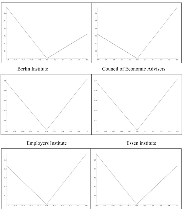
Turning to the inflation forecasts, there are more hindsights to asymmetric loss functions. The Joint Forecast as well as the Council of Economic Advisers have incentives to overestimate inflation, while the Berlin Institute is more likely to underestimate it. Again, visual inspection of the estimated loss functions in Figure 1 confirms the picture given by the formal statistical tests.

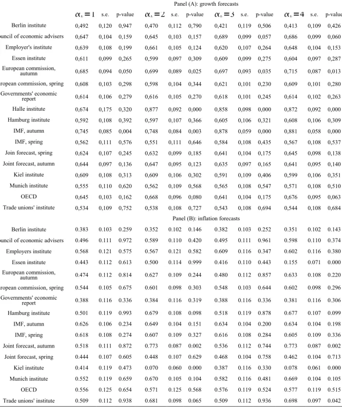
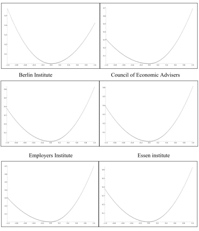
Based on the assumption of a quad-quad loss-function for growth forecasts the broad picture remains more or less unchanged; i.e., there is hardly any convincing evidence for a significant degree of asymmetry across the board of the forecasting institutions (Table 3).

There are some differences from the lin-lin case, however. First, the Berlin Institute appears to have a symmetric loss function in this case. The autumn forecast of the European Commission, the autumn forecast of the IMF; that of the Halle Institute and, again, the forecast of the Council of Economic Advisers show a significant degree of asymmetry, all pointing to incentives to too-optimistic forecasts. Of course, the results for the Halle Institute should be taken with particular caution, due to the very small number of observations (the Institute was founded in 1992).

(12)

As regards the inflation forecasts, four institutions show significant asymmetry: the Joint Forecast in autumn, the Kiel Institute, the Hamburg Institute, and the Trade Unions Institute. All four have a value for the asymmetry parameter, giving incentives for too-high inflation predictions. While this result might meet expectations in all other cases, it might come as a surprise in case of the Trade Unions Institute. However, in all four cases the results have to be taken with great cautiousness since they are not robust against the choice of the instruments (see section 4.2.2 on this issue).

4. Testing for rationality and optimality of a forecast under different loss

functions

4.1 Testing for rationality under a symmetric loss function

Testing the rationality of a forecasts under a symmetric loss function is typically based on two requirements for the forecast: first, the forecast should be unbiased; i.e., no systematic errors should occur – the expected value of the forecast error should not be different from zero. Second, the

forecast should make efficient use of all information available at the forecasting date; i.e., an optimal forecast one should be unable to find any variable, which helps to forecast the errors. In a nutshell, former studies of the rationality of German business cycle forecasts have typically found them unbiased, but not necessarily efficient

To obtain a first insight into the rationality of the forecasts under investigation, we present rationality tests based on a version of the Mincer-Zarnowitz equation (Batchelor and Peel, 1998). In particular, a standard rationality test can be based on estimating the equation:

(13)

y_t__n− y_t__{n ,t}=a₀a₁ y_t__{n ,t}−y_tu_t__n ₍₄₎

As Batchelor and Peel (1998), referring to Christofferson and Diebold (1997) argue, under the null hypothesis of rationality and assuming a symmetric loss function, forecast errors should be

orthogonal to all information known at t, and in particular to the expected change in y. Thus, if the forecast is rational, a₀=0, a₁=0 holds. This is tested with a standard F-test. The results of this task are given in Table 4.

The results, documented in Table 4, give little hints of departures from rationality. In case of the growth forecasts only the Halle Institute shows a significant rejection of the null hypothesis of forecast rationality. This comes as no real surprise, since the Halle Institute was not (re-)founded before 1991, joining the forecast club in 1993. The resulting very short sample reminds to be extremely cautious in interpreting this result. Turning to the inflation forecasts, four institutions show a significant rejection of the null hypothesis. Again, the Halle Institute is among them, but this might be due to the very short sample. Since the IMF forecasts are delivered relatively early as compared to the other forecasts, the non-rationality of these forecasts might be a result of the long forecast horizon. The other results remain to be explained.

(14)

4.2 Rationality testing under an asymmetric loss function

4.2.1 The Batchelor / Peel (1998) approach

One approach to test for forecast rationality under an asymmetric loss function has been proposed by Batchelor and Peel (1998). They start from a so-called linex loss function, which takes the form:

L=

2[expet−et−1] (3)

where  and  are constants and e is the forecast error as described above. The parameter

 determines the degree of asymmetry, while  is a scaling factor. The form of the loss function and the impact of  on the asymmetry of the loss function is illustrated in Figure 3.

 Insert Figure 3 here 

For 0 , losses are approximately exponential for e0 and approximately linear for e0 . If the forecast error is defined as in our case, this defines a situation where underestimations are more costly than overestimations. Conversely, with 0 the function is exponential to the left of the origin of e , and linear to the right. Asymptotically for =0 ,the function coincides with the standard quadratic case.

The standard rationality test resulting in equation (1) may be extended as follows: Batchelor and Peel (1998) argue that under the a linex loss function the optimal forecast has a clearly defined bias.

(15)

expression for the linex loss function. Thus, to test for rationality, an additional term in the test equation is warranted that reflects the expected value of the conditional error variance:

yt1− yt1,t=a0a1 yt1,t−yt

2 Ett21ut1 (4)

Again the null of a rational forecast is represented by the parameter restriction a0=0, a1=0 .

Thus, in empirical testing, Batchelor and Peel (1998) suggest to estimate an ARCH-in-Mean model, tracing back to Engle, Lilian and Roberts (1987). In their original paper, they suggest a GARCH(1,1) model, but argue that the test for rationality does not depend on a specific form of the ARCH-in-Mean term. Hence, in our case, we start with the presumably most simple GARCH(1,1) and use other models only in cases where this model does not fit well to the data. It turned out that, in most cases, using the log for the ARCH-in-Mean term helps to achieve convergence. All in all, the test is performed by estimating the following equations:

yt1− yt1,t=a0a1 yt1,t−yta2Ett21ut1

ut1~N0,t21

_t2_₁=c₁c₂u_t2_₁

c₃_t2

(5)

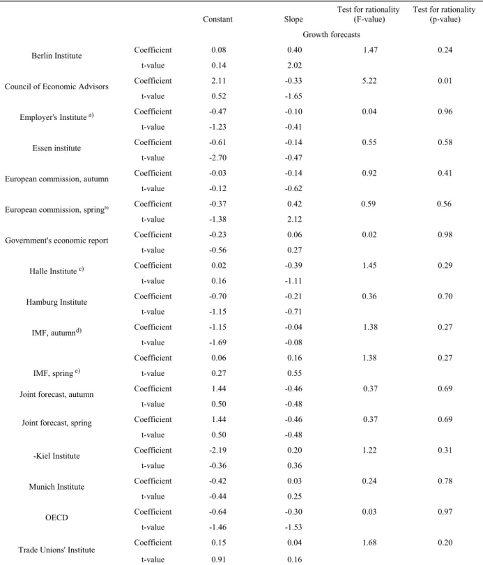
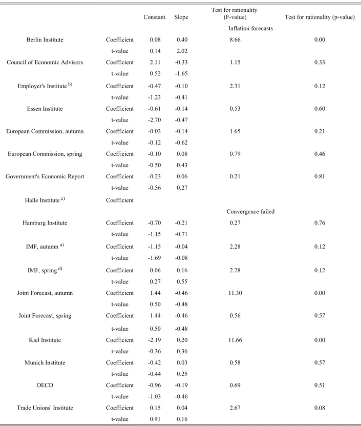
As in the original contribution of Batchelor and Peel (1998) the ARCH-in-Mean terms turn out to be insignificant in most of the cases under investigation here. However, the presence of this term might alter the estimates of the other coefficients in the equation and, thus, the results of testing for

(16)

rationality, namely a₀=0, a₁=0 . The results presented in Table 5 suggest that in virtually all cases the null of rationality cannot be rejected for the growth forecasts considered in this paper. The results changes, when considering the inflation forecast errors; however, again the results do not differ qualitatively from the case of a symmetric loss function.

 Insert Table 5 here  4.2.2 The Elliot et al. (2005) approach

Elliot et al. (2005) suggest a test of the joint null hypothesis of forecast rationality and the underlying loss function. Under the null hypothesis the test statistic is:

[

]

[

]

2 1 1 1 1 1 1 1 1 ' 1 1 1 1 1 1 ~ ˆ ) 0 ˆ ( 1 ˆ ˆ ) 0 ˆ ( 1 1 0 0 − − + + + + − + = − − + + + + − + = _Χ                     ₋ _< ₋ ₋ ⋅       ₋ _< ₋ ₋ =

∑

d p t t T t t T t t p t t T t t T t t y y y y S y y y y T J α υ α υ τ τ τ τ (6)

Hence, a rejection of the hypothesis might be due to irrationality of the forecast or due to the rejection of the functional form of the loss function. The results for our data at hand are given in Table 6.

In case of growth forecasts and the lin-lin setting, the null hypothesis has to be rejected only in very few cases. In particular, for the IMF (autumn forecast), the OECD, and the Council of Economic Advisers the hypothesis is not supported by the data. However, in none of the three cases, the result

(17)

the forecasts or the necessity of a different loss function are not convincing. By contrast, the results for the inflation forecasts lead to a rejection of the null hypothesis for virtually any of the institutions under investigation. Given the point estimates of the asymmetry parameter reported in Section 3, one might suspect that the rejection is due to the failure of the rationality hypothesis rather than due to the assumption of a particular loss function, but formally the test does not tell anything about this. However, the results reported for similar tests based on the assumption of a quad-quad loss function yield a similar picture: again, there are very few results, if any at all, pointing to the rejection of the null for the growth forecasts, but the inflation forecasts fail to achieve rationality under this

particular loss function. Hence, all in all, the rationality of growth forecasts is generally supported by the J-test while the rationality of the inflation forecasts is much more in doubt. It is noteworthy that the the null of rationality is frequently rejected, when the lagged forecast errors are used as

instruments which implies that the orthogonality condition between actual and lagged forecast errors does not hold. This finding corresponds to the high positive autocorrelation of the inflation forecast errors reported in Table 1.

4.2.3 Testing the properties of an optimal forecast under a general loss function

Recently, Patton and Timmerman (2007) have proposed a set of tests for forecast optimality under a generalized loss function. Under the joint hypothesis that the forecasts are optimal, the loss function is solely a function of the forecast error, and the dynamics of the predicted variable show no dynamics beyond the conditional mean, the forecast errors should be homoscedastic (Patton and Timmermann 2007: 12). This hypothesis may easily be tested using the procedure proposed by Engle (1982). In particular, the following equation is estimated:

(18)

et2=a0a1et2−1aLet2−Lut (7)

and the hypothesis a₁=a₂==a_L=0 is tested. If rejected, the test result implies that either the forecast is not optimal or one of the other assumptions (no dynamics beyond the conditional mean and loss function depending solely on the forecast errors) does not hold. The results for the German business cycle forecasts are presented in Table 7.

With the exception of three forecasting institutions and only in the case of their respective inflation forecast we are never able to reject the hypothesis – even at the 10 per cent level. According to that criterion there is no evidence for heteroscedastic forecast errors. Hence, the forecasts have to be considered as optimal insofar as the loss function is solely a function of the forecast errors.

To test the assumption of no dynamics beyond the conditional mean directly; however, it is

warranted to model the conditional mean. We do this by estimating a simple ARMA(1,1) model of output growth and inflation respectively.5_{In both cases, the model removes all autocorrelation up to}

5 _{The results for the estimation for output growth yields} yt=0.99978

274.5

yt−1−0.9775

−5.11

ut−1ut _{(t-values in brackets). A}

test for remaining autocorrelation yields a p-value of 0.66. The respective equation for inflation gives the following results yt=0.939719.84

yt−10.3137

2.30

ut−1ut

(19)

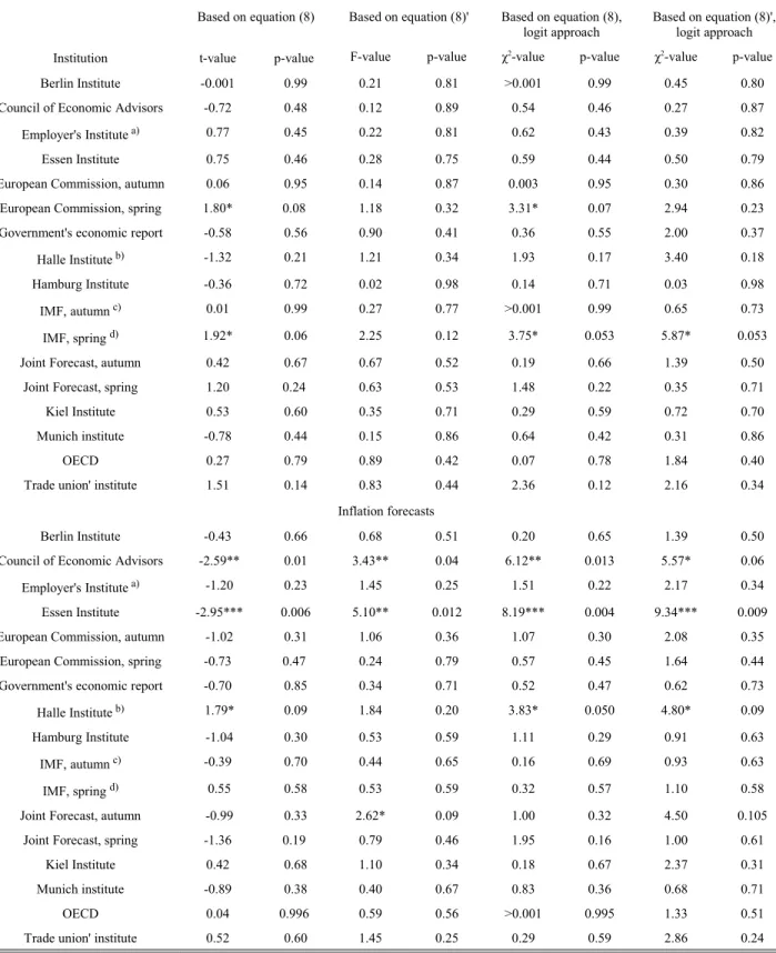
significance of the squared residuals of these equations. Thus, we cannot confirm any evidence against the optimality of the forecasts under investigation. Furthermore, Patton and Timmermann (2007) suggest to rely on a quantile-related approach. This test relies on an indicator function:

I_t_₁=1y_t_₁ y_t_₁ . With this variable at hand, the following equations are estimated respectively:

I_t_₁=a₀a₁y_t_₁u_t_₁ (8)

It1=a0a1yt1a2Itut1 (8')

The null hypothesis is given by a₁=0 and a₁=a₂=0 , respectively. If rejected, the test implies either the rejection of conditional variance dynamics in the data generating process of GDP growth or inflation, or a rejection of the optimality of the forecast at hand and any loss function which is at least homogeneous in the forecast error. The results for the German data set are given in Table 8. As mentioned in Patton and Timmermann (2007: 9) it is also possible to estimate equation (8) and (8’) using a logit-approach. We have done so; the results are also presented in Table 8. All in all, we find evidence against the optimality of the forecast errors in very few cases only. In particu-lar, the output forecasts appear to be rational. As regards the inflation forecast there are two cases with a significant violation of the optimality requirements in case of OLS estimation. However, even in these cases the finding is not confirmed by the logit estimation.

(20)

5. Conclusion

The paper analyses the degree of asymmetry of German business cycle forecasts, namely growth and inflation forecasts covering the time span from 1970 to 2007 and up to 17 different forecasts. We find the forecasts to be mostly symmetric with only few exceptions. The point estimates of the degree of asymmetry are not systematic in any respect: some forecasters seem to have incentives for too-pessimistic forecasts, some others for too-optimistic forecasts. The results appear to be not fully robust against the choice of the instruments warranted to estimate the loss function with a GMM approach. We also investigate the rationality of the forecasts at hand. To this end, we do not

exclusively rely on the assumption of a symmetric loss function, but make use of approaches based on an asymmetric or even flexible loss function. In a nutshell, we find that neither a specifically asymmetric loss function nor the assumption of a generalized loss function alter the findings ob-tained under a symmetric loss function by very much, though the results of the test proposed by Elliot et al. (2005) give some contrary results for inflation forecasts.

Given the results of this paper, some further research may be required. First, is must be checked, whether data with a higher frequency may alter the results. Having more data may help the estimate the asymmetry parameter with greater precision and, hence, lead to more cases with a significant degree of asymmetry. Second, it may be worthwhile to try to estimate the asymmetry parameter for government in order to compare it with the values for the forecasters. It is plausible to assume that the political authorities have different loss functions than do forecasters; which may, in turn, explain some of the bad image of business cycle forecasts in the public opinion.

(21)

References

Artis, M., and M. Marcelino (2001). Fiscal Forecasting: The track record of the IMF, OCED, and

EC. Econometrics Journal 4: 20-36.

Batchelor, R., and D. Peel (1998). Rationality testing under asymmetric loss. Economics Letters 61: 49-54.

Blinder, A.S.(1998). Central Banking in Theory and Practice. Cambridge: MIT Press.

Christodoulakis, G., and M. Mamatzakis (2008). An Assessment of the EU Growth Forecasts under Asymmetric Preferences, Journal of Forecasting, 27: 483-492.

Christodoulakis, G., and M. Mamatzakis (2009). Assessing the Prudence of Economic Forecasts in the EU, Journal of Applied Econometrics, forthcoming.

Christoffersen, P.F., and F.X. Diebold, (1997). Optimal Prediction under Asymmetric Loss.

Econo-metric Theory 13: 808-817.

Döpke, J. (2000). Haben Konjunkturprognosen einen politischen Bias? Schmollers Jahrbuch -

Zeits-chrift für Wirtschafts- und Sozialwissenschaften 120 (2000): 587-620.

Döpke, J., and U. Fritsche (2006). Growth and inflation forecasts in Germany: a panel-based assess-ment of accuracy and dispersion. Empirical Economics 31: 777-798.

Elliot, G, I. Komunjer, and A. Timmermann (2005). Estimation and testing of forecast rationality un-der flexible loss. Review of Economic Studies 72: 1107-1125.

Elliot, G, I. Komunjer, and A. Timmermann (2008). Biases in Macroeconomic Forecasts: Irrational-ity or Asymmetric Loss? Journal of European Economic Association, 2008, 6(1), 122-15. Engle, R. F., Lilien, D. M., and R. P. Robins (1987). Estimating time-varying premia in the term

structure: the ARCH-M model. Econometrica 55: 391-407.

Engle, R.F. (1982). Autoregressive Conditional Heteroskedasticity With Estimates of the Variance of U.K. Inflation. Econometrica 50, 987-1008.

Fildes, R., and Stekler, H.O. (2002). The state of macroeconomic forecasting. Journal of

Macroeco-nomics 24: 435-468.

Granger, C.W.J. (1999). Outline of Forecast Theory Using Generalized Cost Functions. Spanish

Economic Review 1: 161-173.

Hansen, B.E., and K.D. West (2002). Generalized Methods of Moments and Macroeconomics.

Journal of Business & Economics Statistics 20: 460-490.

Miersch, M. (2008). Wir prognostizieren uns zu Tode.

http://debatte.welt.de/kommentare/103709/wir+prognostizieren+uns+zu+tode

Patton, A.J., and A. Timmermann (2007). Testing forecast optimality under unknown loss. Journal of American Statistical Association, 2007: 102, 1172-1184.

(22)

Table 1: Descriptive Statistics for forecast errors, 1970 to 2007

Institution Mean error Mean absolute _error _{squared error}Root mean _coefficientTheil's

Autocorrelation coefficient of forecast

error (p-value) Growth forecasts

Berlin Institute 0.04 1.02 1.47 0.61 0.08 (0.63)

Council of Economic Advisors -0.29 1.01 1.42 0.59 0.03 (0.85)

Employer's Institute a) _-0.27 _1.17 _1.67 _0.69 _{-0.25 (0.15)}

Essen Institute -0.23 1.00 1.31 0.54 0.11 (0.53)

European Commission, autumn -0.42 1.18 1.62 0.67 -0.03 (0.87)

European Commission, spring -0.19 0.78 1.08 0.45 0.14 (0.40)

Government's Economic Report -0.21 0.95 1.37 0.57 -0.14 (0.41)

Halle Institute b) -0.29 0.68 0.92 0.38 -0.37 (0.20)

Hamburg Institute -0.15 0.95 1.34 0.56 -0.08 (0.66)

IMF, autumn c) _-0.63 _1.33 _1.77 _0.73 _{0.01 (0.97)}

IMF, spring d) _-0.12 _0.86 _1.19 _0.50 _{0.29* (0.08)}

Joint Forecast, autumn -0.32 1.19 1.61 0.67 -0.01 (0.96)

Joint Forecast, spring _-0.20 _0.80 _1.14 _0.47 _{-0.01 (0.97)}

Kiel Institute -0.20 1.04 1.50 0.62 0.03 (0.87)

Munich Institute -0.09 0.93 1.29 0.53 -0.13 (0.45)

OECD -0.30 1.05 1.53 0.63 -0.08 (0.63)

Trade Union' Institute -0.08 1.13 1.55 0.64 -0.05 (0.75)

Inflation forecasts

Berlin Institute 0.19 0.70 0.93 0.94 0.36** (0.03)

Council of Economic Advisors 0.03 0.71 0.94 0.96 0.47*** (0.003)

Employer's Institute a) _-0.03 _0.52 _0.74 _0.75 _{0.20 (0.24)}

Essen Institute 0.09 0.60 0.83 0.84 0.55*** (0.001)

European Commission, autumn 0.07 0.68 0.93 0.95 0.56*** (0.0003)

European Commission, spring -0.02 0.37 0.47 0.48 0.25 (0.12)

Government's Economic Report 0.16 0.59 0.88 0.89 0.38** (0.019)

Halle Institute b) _0.02 _0.50 _0.69 _0.70 _{0.22 (0.46)}

Hamburg Institute 0.03 0.64 0.92 0.93 0.47*** (0.004)

IMF, autumn c) _-0.10 _0.67 _0.91 _0.92 _{0.31* (0.07)}

IMF, spring d) -0.15 0.58 0.83 0.84 0.42** (0.017)

Joint Forecast, autumn 0.02 0.77 1.03 1.05 0.58*** (0.002)

Joint Forecast, spring _0.05 _0.44 _0.58 _0.59 _{0.22 (0.20)}

Kiel Institute 0.19 0.76 1.15 1.17 0.62*** (>0.001)

Munich Institute -0.03 0.59 0.84 0.85 0.24 (0.16)

OECD -0.04 0.56 0.76 0.78 0.19 (0.29)

Trade Union' Institute 0.02 0.78 1.05 1.07 0.55*** (0.004)

Notes: a) 1972 to 2007; b) 1993 to 2007; c) 1973 to 2007; d) 1971 to 2007. e) p-value refers to a two sided test of the null hypothesis of an autorcorrelation coefficient equal to zero. *** (**, *) denotes rejection of the null at the 1 (5, 10) percent level.

(23)

Panel (A): growth forecasts

_k=1 s.e. p-value __k₌2 s.e. p-value __k₌3 s.e. p-value __k₌4 s.e. p-value Berlin institute 0.324 0.077 0.022 0.319 0.077 0.0018 0.324 0.077 0.0018 0.318 0.077 0.0017 Council of Economic Advisers 0.595 0.081 0.241 0.595 0.081 0.241 0.639 0.079 0,079 0.639 0.079 0,079 Employer's Institute 0.571 0.084 0.393 0.575 0.084 0.372 0.573 0.084 0.383 0.578 0.083 0.351 Essen Institute 0.568 0.081 0.407 0.568 0.081 0.407 0.578 0.081 0.340 0.578 0.081 0.339 European Commission, autumn 0.541 0.082 0.621 0.542 0.082 0.611 0.547 0.082 0.563 0.550 0.082 0.545 European Commission, spring 0.486 82 0.869 0.486 0.082 0.869 0.486 0.082 0.869 0.486 0.082 0.869 Governments' Economic Report 0.514 0.082 0.869 0.514 0.082 0.866 0.515 0.082 0.854 0.516 0.082 0.850 Halle Institute 0.571 0.132 0.589 0.572 0.132 0.588 0.585 0.132 0.519 0.586 0.132 0.515 Hamburg Institute 0.432 0.081 0.407 0.432 0.081 0.403 0.428 0.081 0.373 0.427 0.081 0.370 IMF, autumn 0.588 0.084 0.296 0.588 0.084 0.296 0.624 0.083 0.136 0.624 0.083 0.136 IMF, spring 0.444 0.083 0.502 0.441 0.083 0.475 0.444 0.083 0.496 0.441 0.083 0.472 Join Forecast, spring 0.514 0.082 0.869 0.514 0.082 0.869 0.514 0.082 0.869 0.514 0.082 0.869 Joint Forecast, autumn 0.486 0.082 0.869 0.486 0.082 0.866 0.485 0.082 0.857 0.485 0.082 0.851 Kiel Institute 0.486 0.082 0.869 0.486 0.082 0.869 0.486 0.082 0.862 0.486 0.082 0.861 Munich institute 0.459 0.082 0.621 0.459 0.082 0.620 0.459 0.082 0.619 0.459 0.082 0.618 OECD 0.568 0.081 0.407 0.571 0.081 0.383 0.580 0.081 0.326 0.585 0.081 0.294 Trade Unions' Institute 0.486 0.082 0.869 0.486 0.082 0.866 0.485 0.082 0.857 0.484 0.082 0.857

Panel (B): inflation forecasts

Berlin institute 0.378 0.080 0.127 0.333 0.077 0.031 0.378 0.080 0.125 0.327 0.077 0.025 Council of Economic Advisers 0.649 0.078 0.058 0.704 0.075 0.007 0.678 0.077 0.021 0.714 0.074 0.004 Employer's Institute 0.514 0.084 0.866 0.515 0.084 0.861 0.515 0.084 0.859 0.515 0.084 0.856 Essen Institute 0.514 0.082 0.869 0.533 0.082 0.688 0.517 0.082 0.832 0.535 0.082 0.671 European Commission, autumn 0.568 0.081 0.407 0.602 0.080 0.206 0.568 0.081 0.406 0.606 0.080 0.189 European Commission, spring 0.432 0.081 0.407 0.428 0.081 0.374 0.432 0.081 0.406 0.428 0.081 0.374 Governments' Economic Report 0.432 0.081 0.407 0.416 0.081 0.297 0.432 0.081 0.407 0.414 0.081 0.291 Halle Institute Hamburg Institute 0.568 0.081 0.407 0.588 0.081 0.274 0.569 0.081 0.400 0.588 0.081 0.274 IMF, autumn 0.441 0.085 0.490 0.427 0.085 0.392 0.441 0.085 0.490 0.427 0.085 0.389 IMF, spring 0.528 0.083 0.738 0.531 0.083 0.711 0.528 0.083 0.738 0.531 0.083 0.711 Join Forecast, spring 0.649 0.078 0.058 0.702 0.075 0.007 0.650 0.078 0.056 0.710 0.075 0.005 Joint Forecast, autumn 0.405 0.081 0.241 0.388 0.080 0.160 0.397 0.080 0.199 0.382 0.080 0.139 Kiel Institute 0.432 0.081 0.407 0.412 0.081 0.276 0.429 0.081 0.382 0.392 0.080 0.178 Munich institute 0.541 0.082 0.621 0.546 0.082 0.578 0.541 0.082 0.614 0.546 0.082 0.575 OECD 0.600 0.089 0.264 0.622 0.089 0.169 0.603 0.089 0.250 0.630 0.088 0.141 Trade Unions' Institute 0.514 0.082 0.869 0.519 0.082 0.819 0.515 0.082 0.856 0.523 0.082 0.780

(24)

Table 3: Evidence for an asymmetric loss function, quad-quad loss function

Panel (A): growth forecasts

_k=1 s.e. p-value __k₌2 s.e. p-value __k₌3 s.e. p-value __k₌4 s.e. p-value Berlin institute 0,492 0,120 0,947 0,470 0,112 0,790 0,421 0,119 0,506 0,413 0,109 0,426 Council of economic advisers 0,647 0,104 0,159 0,645 0,103 0,157 0,689 0,099 0,057 0,686 0,099 0,060 Employer's institute 0,639 0,108 0,199 0,661 0,105 0,124 0,620 0,107 0,264 0,648 0,104 0,153 Essen institute 0,611 0,099 0,265 0,599 0,097 0,309 0,609 0,099 0,275 0,604 0,097 0,287 European commission,

autumn 0,685 0,094 0,050 0,699 0,089 0,025 0,697 0,093 0,035 0,715 0,087 0,013 European commission, spring 0,608 0,103 0,298 0,598 0,104 0,344 0,621 0,101 0,230 0,609 0,101 0,280

Governments' economic report 0,614 0,106 0,279 0,616 0,105 0,270 0,618 0,101 0,245 0,614 0,102 0,263 Halle institute 0,674 0,175 0,320 0,877 0,092 0,000 0,858 0,098 0,000 0,872 0,092 0,000 Hamburg institute 0,592 0,108 0,392 0,597 0,107 0,366 0,605 0,106 0,321 0,608 0,106 0,309 IMF, autumn 0,745 0,085 0,004 0,748 0,084 0,003 0,878 0,059 0,000 0,881 0,058 0,000 IMF, spring 0,562 0,111 0,576 0,551 0,111 0,646 0,584 0,108 0,435 0,567 0,108 0,537 Join forecast, spring 0,624 0,107 0,245 0,632 0,099 0,185 0,641 0,104 0,175 0,645 0,098 0,138 Joint forecast, autumn 0,644 0,097 0,136 0,647 0,095 0,123 0,635 0,097 0,165 0,641 0,095 0,140 Kiel institute 0,609 0,108 0,313 0,609 0,106 0,302 0,591 0,109 0,406 0,599 0,106 0,351 Munich institute 0,555 0,110 0,620 0,562 0,109 0,568 0,565 0,108 0,547 0,571 0,108 0,510 OECD 0,645 0,103 0,162 0,668 0,096 0,080 0,641 0,104 0,175 0,676 0,095 0,063 Trade unions' institute 0,534 0,109 0,752 0,538 0,108 0,727 0,543 0,108 0,694 0,544 0,108 0,684

Panel (B): inflation forecasts

Berlin institute 0.383 0.103 0.259 0.352 0.102 0.146 0.382 0.103 0.252 0.351 0.102 0.143 Council of economic advisers 0.496 0.111 0.972 0.589 0.110 0.420 0.495 0.111 0.961 0.598 0.110 0.374 Employers institute 0.568 0.121 0.575 0.567 0.121 0.582 0.609 0.116 0.347 0.602 0.116 0.380 Essen institute 0.443 0.112 0.613 0.500 0.114 0.999 0.416 0.110 0.443 0.155 0.071 0.000 European commission,

autumn 0.474 0.112 0.814 0.627 0.109 0.244 0.480 0.112 0.857 0.633 0.108 0.220 European commission, spring 0.544 0.105 0.675 0.601 0.098 0.303 0.548 0.103 0.644 0.602 0.098 0.296

Governments' economic

report 0.388 0.116 0.336 0.384 0.116 0.319 0.388 0.116 0.336 0.381 0.116 0.306 Hamburg institute 0.501 0.119 0.993 0.679 0.108 0.098 0.518 0.119 0.878 0.677 0.107 0.099 IMF, autumn 0.626 0.106 0.234 0.649 0.104 0.151 0.634 0.104 0.200 0.634 0.104 0.198 IMF, spring 0.618 0.108 0.274 0.607 0.109 0.327 0.616 0.108 0.284 0.605 0.109 0.336 Joint forecast, autumn 0.518 0.111 0.872 0.773 0.087 0.002 0.536 0.112 0.744 0.773 0.087 0.002 Joint forecast, spring 0.444 0.107 0.605 0.448 0.107 0.629 0.468 0.104 0.758 0.462 0.104 0.713 Kiel institute 0.414 0.119 0.473 0.070 0.060 0.000 0.387 0.116 0.330 0.078 0.061 0.000 Munich institute 0.552 0.119 0.659 0.670 0.105 0.104 0.582 0.116 0.481 0.669 0.104 0.105 OECD 0.556 0.125 0.654 0.571 0.125 0.568 0.576 0.119 0.524 0.577 0.119 0.515 Trade unions' institute 0.509 0.112 0.938 0.681 0.098 0.065 0.509 0.112 0.936 0.698 0.097 0.042

(25)

1970 to 2007

Constant Slope

Test for rationality (F-value)

Test for rationality (p-value) Growth forecasts Berlin Institute 0.015 (0.06) 0.081 (0.48) 0.118 0.89

Council of Economic Advisors

-0.293 (-1.20) 0.031 (0.18) 0.825 0.45 Employer's Institute a) -0.398 (-1.41) -0.247 (-1.47) 1.758 0.19 Essen Institute (-0.89)-0.199 (0.62)0.107 0.727 0.49

European Commission, autumn (-1.64)-0.456 (-0.16)-0.027 1.388 0.26

European Commission, spring

-0.140 (-0.77)

0.142 (0.86)

0.808 0.46

Government's Economic Report

-0.253 (-1.09) -0.142 (-0.84) 0.818 0.45 Halle Institute b) -0.332 (-1.35) -0.352 (-1.37) 1.397 0.28 Hamburg Institute -0.190 (-0.83) -0.075 (-0.45) 0.408 0.67 IMF, autumn c) -0.660 (-2.08) 0.007 (0.04) 2.55 0.09 IMF, spring d) _(-0.34)-0.067 _(1.79)0.295 1.756 0.19

Joint Forecast, autumn

-0.349 (-1.27)

-0.009 (-0.05)

0.829 0.45

Joint Forecast, spring

-0.202 (-1.04) -0.005 (-0.03) 0.594 0.58 Kiel Institute -0.221 (-0.87) 0.027 (0.16) 0.416 0.66 Munich Institute -0.116 (-0.53) -0.127 (0.76) 0.399 0.67 OECD -0.345 (-1.32) -0.082 (-0.49) 0.895 0.42

Trade Unions' Institute

-0.086 (-0.33) -0.055 (-0.32) 0.098 0.91 a)1972 to 2007; b) 1993 to 2007; c) 1973 to 2007; d) 1971 to 2007.

(26)

Table 4: continued

Constant Slope

Test for rationality (p-value) Inflation forecasts Berlin Institute 0.096 (0.67) 0.356 (2.31) 3.296 0.049

Council of Economic Advisors

-0.012 (-0.86) 0.459 (3.12) 4.874 0.01 Employer's Institute a) _(-0.50)-0.061 _(1.20)0.196 0.865 0.43 Essen Institute (0.10)0.012 (3.86)0.536 7.617 0.002

European Commission, autumn

0.001 (0.01)

0.547 (4.00)

8.030 0.001

European Commission, spring

-0.022 (-0.28)

0.259 (1.56)

1.302 0.28

Government's Economic Report

0.073 (0.53) 0.376 (2.45) 3.459 0.04 Halle Institute b) 0.046 (0.23) 0.219 (0.76) 0.321 0.73 Hamburg Institute -0.016 (-0.11) 0.458 (3.12) 4.875 0.014 IMF, autumn c) _(-0.89)-0.127 _(1.86)0.289 2.344 0.11 IMF, spring d) _(-0.52)-0.068 _(2.66)0.413 4.11 0.025

Joint Forecast, autumn

-0.038 (-0.27)

0.563 (4.23)

8.973 0.001

Joint Forecast, spring

0.042 (0.43) 0.221 (1.33) 1.011 0.374 Kiel Institute 0.015 (0.10) 0.581 (4.67) 11.278 0.0001 Munich Institute -0.054 (-0.39) 0.231 (1.44) 1.134 0.33 OECD -0.041 (-0.30) 0.194 (1.08) 0.656 0.524

Trade Unions' Institute (-0.09)-0.014 (3.92)0.547 7.96 0.002

(27)

Table 5: Test for rationality of the forecasts under an asymmetric loss function

(Batchelor/Peel approach), 1970 to 2007

Constant Slope

Test for rationality (p-value) Growth forecasts

Berlin Institute Coefficient 0.08 0.40 1.47 0.24

t-value 0.14 2.02

Council of Economic Advisors Coefficient 2.11 -0.33 5.22 0.01

t-value 0.52 -1.65

Employer's Institute a) Coefficient -0.47 -0.10 0.04 0.96

t-value -1.23 -0.41

Essen institute Coefficient -0.61 -0.14 0.55 0.58

t-value -2.70 -0.47

European commission, autumn Coefficient -0.03 -0.14 0.92 0.41

t-value -0.12 -0.62

European commission, springb) Coefficient -0.37 0.42 0.59 0.56

t-value -1.38 2.12

Government's economic report Coefficient -0.23 0.06 0.02 0.98

t-value -0.56 0.27

Halle Institute c) Coefficient 0.02 -0.39 1.45 0.29

t-value 0.16 -1.11

Hamburg Institute Coefficient -0.70 -0.21 0.36 0.70

t-value -1.15 -0.71

IMF, autumnd) Coefficient -1.15 -0.04 1.38 0.27

t-value -1.69 -0.08

IMF, spring e)

Coefficient 0.06 0.16 1.38 0.27

t-value 0.27 0.55

Joint forecast, autumn Coefficient 1.44 -0.46 0.37 0.69

t-value 0.50 -0.48

Joint forecast, spring Coefficient 1.44 -0.46 0.37 0.69

t-value 0.50 -0.48

-Kiel Institute Coefficient -2.19 0.20 1.22 0.31

t-value -0.36 0.36

Munich Institute Coefficient -0.42 0.03 0.24 0.78

t-value -0.44 0.25

OECD Coefficient -0.64 -0.30 0.03 0.97

t-value -1.46 -1.53

Trade Unions' Institute Coefficient 0.15 0.04 1.68 0.20

t-value 0.91 0.16

a)1972 to 2007; b) 1993 to 2007; c) 1973 to 2007; d) 1971 to 2007. e) Convergence could only be achieved after eliminating the year 1975 by a dummy variable in the mean equation.

(28)

Table 5: continued

Constant Slope

Test for rationality

(F-value) Test for rationality (p-value) Inflation forecasts

Berlin Institute Coefficient 0.08 0.40 8.66 0.00

t-value 0.14 2.02

Council of Economic Advisors Coefficient 2.11 -0.33 1.15 0.33

t-value 0.52 -1.65

Employer's Institute b) _Coefficient _-0.47 _-0.10 _2.31 _0.12

t-value -1.23 -0.41

Essen Institute Coefficient -0.61 -0.14 0.53 0.60

t-value -2.70 -0.47

European Commission, autumn Coefficient -0.03 -0.14 1.65 0.21

t-value -0.12 -0.62

European Commission, spring Coefficient -0.10 0.08 0.79 0.46

t-value -0.50 0.43

Government's Economic Report Coefficient -0.23 0.06 0.21 0.81

t-value -0.56 0.27 Halle Institute c) _Coefficient

Convergence failed

Hamburg Institute Coefficient -0.70 -0.21 0.27 0.76

t-value -1.15 -0.71

IMF, autumn a) Coefficient -1.15 -0.04 2.28 0.12

t-value -1.69 -0.08

IMF, spring d) _Coefficient _0.06 _0.16 _2.28 _0.12

t-value 0.27 0.55

Joint Forecast, autumn Coefficient 1.44 -0.46 11.30 0.00

t-value 0.50 -0.48

Joint Forecast, spring Coefficient 1.44 -0.46 0.56 0.57

t-value 0.50 -0.48

Kiel Institute Coefficient -2.19 0.20 11.66 0.00

t-value -0.36 0.36

Munich Institute Coefficient -0.42 0.03 0.58 0.57

t-value -0.44 0.25

OECD Coefficient -0.96 -0.19 0.69 0.51

t-value -1.03 -0.46

Trade Unions' Institute Coefficient 0.15 0.04 2.67 0.08

t-value 0.91 0.16

(29)

2007

J-test k=2 p-value J-test k=3 p-value J-test k=4 p-value Panel (A): Growth forecasts

Berlin Institute 0,57 0,45 0,03 0,87 0,69 0,71

Council of Economic Advisers 0,01 0,93 5,90 0,02 5,90 0,05

Employers Institute 0,76 0,39 0,35 0,56 1,44 0,49

Essen Institute 0,00 0,98 2,38 0,12 2,39 0,30

European Commission, autumn 0,51 0,48 2,65 0,10 3,35 0,19

European Commission, spring 0,05 0,83 0,05 0,83 0,08 0,96

Government Report 0,48 0,49 2,01 0,16 2,45 0,29

Halle Institute 0,01 0,91 1,11 0,29 1,16 0,56

Hamburg Institute 0,13 0,72 1,24 0,27 1,36 0,51

IMF, autumn 0,00 0,98 4,88 0,03 4,89 0,09

IMF, spring 1,08 0,30 0,27 0,60 1,19 0,55

Joint Forecast, autumn 0,45 0,50 1,60 0,21 2,25 0,33

Joint Forecast, spring 0,02 0,89 0,02 0,90 0,04 0,98

Kiel Institute 0,04 0,84 1,02 0,31 1,19 0,55

Munich Institute 0,03 0,88 0,11 0,74 0,13 0,94

OECD 0,90 0,34 2,83 0,09 3,80 0,15

Trade Unions' Institute 0,43 0,51 1,63 0,20 2,50 0,29

Panel (b): Inflation forecasts

Employer's Institute 0,57 0,45 0,87 0,35 1,14 0,56

Essen Institute 10,90 0,00 4,11 0,04 11,32 0,00

IMF, autumn 3,22 0,07 0,00 0,97 3,32 0,19

IMF, spring 1,75 0,19 0,00 0,97 1,77 0,41

Kiel Institute 4,33 0,04 0,92 0,34 6,94 0,03

OECD 2,69 0,10 0,39 0,53 3,44 0,18

(30)

Table 6, cont: Joint test for forecast rationality and loss function (J-test), quad-quad function, 1970 to 2007

J-test k=2 p-value J-test k=3 p-value J-test k=4 p-value Panel (A): Growth forecasts

Employers Institute 1,62 0,20 0,86 0,36 1,96 0,38

Essen Institute 0,28 0,60 1,79 0,18 1,81 0,40

Halle Institute 1,49 0,22 1,31 0,25 1,58 0,45

IMF, autumn 0,07 0,79 5,54 0,02 5,59 0,06

IMF, spring 2,59 0,11 1,02 0,31 2,89 0,24

Kiel Institute 0,00 0,99 3,63 0,06 3,72 0,16

OECD 0,43 0,51 1,28 0,26 2,07 0,36

Trade Unions' Institute 0,09 0,77 2,07 0,15 2,08 0,35

Panel (B): Inflation forecasts

Employer's Institute 1,33 0,25 1,81 0,18 2,02 0,36

Essen Institute 6,82 0,01 3,92 0,05 10,11 0,01

Government Report 3,46 0,06

1,27E-005

1 4,67 0,1

IMF, autumn 2,96 0,09 0,21 0,65 3,38 0,18

IMF, spring 2,66 0,1 1,73 0,19 3,15 0,21

Kiel Institute 8,7 0 1,37 0,24 10,37 0,01

OECD 0,93 0,34 0,21 0,65 0,93 0,63

(31)

Institution F-value p-value Growth forecasts

Berlin Institute 0.37 0.70

Council of Economic Advisors 0.01 0.99

Employer's Institute a) 0.01 0.99

Essen Institute 0.38 0.68

European Commission, autumn 0.60 0.56

European Commission, spring 0.001 0.99

Government's Economic Report 0.24 0.79

Halle Institute b) 0.07 0.80

Hamburg Institute 0.16 0.85

IMF, autumn c) 0.25 0.78

IMF, spring d) _0.13 _0.88

Joint Forecast, autumn 0.27 0.77

Joint Forecast, spring 0.15 0.86

Kiel Institute 0.24 0.79

Munich Institute 0.02 0.98

OECD 1.01 0.37

Trade Unions' Institute 0.70 0.60

Inflation forecasts

Berlin Institute 0.46 0.63

Council of Economic Advisors 0.70 0.51

Employer's Institute b) 0.12 0.88

Essen Institute 3.00 0.06

European Commission, autumn 1.82 0.18

European Commission, spring 0.89 0.42

Government's Economic Report 3.11* 0.05

Halle Institute c) 3.25* 0.08

Hamburg Institute 0.28 0.76

IMF, autumn a) 0.11 0.90

IMF, spring d) 2.12 0.14

Joint Forecast, autumn 0.75 0.48

Joint Forecast, spring 0.35 0.71

Kiel Institute 3.12* 0.06

Munich Institute 0.06 0.94

OECD 0.64 0.53

Trade union' institute 2.29 0.12

*** (**, *) denotes rejection of the null hypothesis at the 1 (5,10) percent level. a) 1973 to 2007; 1972 to 2007; c) 1993 to 2007; d) 1971 to 2007

(32)

Table 8: Test for forecast optimality under a generalized loss function, 1970 to

2007

Growth forecasts

Based on equation (8) Based on equation (8)' Based on equation (8), logit approach

Based on equation (8)', logit approach Institution t-value p-value F-value p-value χ2_-value _p-value _χ2_-value _p-value

Berlin Institute -0.001 0.99 0.21 0.81 >0.001 0.99 0.45 0.80

Council of Economic Advisors -0.72 0.48 0.12 0.89 0.54 0.46 0.27 0.87

Employer's Institute a) 0.77 0.45 0.22 0.81 0.62 0.43 0.39 0.82

Essen Institute 0.75 0.46 0.28 0.75 0.59 0.44 0.50 0.79

European Commission, autumn 0.06 0.95 0.14 0.87 0.003 0.95 0.30 0.86

European Commission, spring 1.80* 0.08 1.18 0.32 3.31* 0.07 2.94 0.23

Government's economic report -0.58 0.56 0.90 0.41 0.36 0.55 2.00 0.37

Halle Institute b) -1.32 0.21 1.21 0.34 1.93 0.17 3.40 0.18

Hamburg Institute -0.36 0.72 0.02 0.98 0.14 0.71 0.03 0.98

IMF, autumn c) 0.01 0.99 0.27 0.77 >0.001 0.99 0.65 0.73

IMF, spring d) 1.92* 0.06 2.25 0.12 3.75* 0.053 5.87* 0.053

Joint Forecast, autumn 0.42 0.67 0.67 0.52 0.19 0.66 1.39 0.50

Joint Forecast, spring 1.20 0.24 0.63 0.53 1.48 0.22 0.35 0.71

Kiel Institute 0.53 0.60 0.35 0.71 0.29 0.59 0.72 0.70

Munich institute -0.78 0.44 0.15 0.86 0.64 0.42 0.31 0.86

OECD 0.27 0.79 0.89 0.42 0.07 0.78 1.84 0.40

Trade union' institute 1.51 0.14 0.83 0.44 2.36 0.12 2.16 0.34

Inflation forecasts

Berlin Institute -0.43 0.66 0.68 0.51 0.20 0.65 1.39 0.50

Council of Economic Advisors -2.59** 0.01 3.43** 0.04 6.12** 0.013 5.57* 0.06

Employer's Institute a) -1.20 0.23 1.45 0.25 1.51 0.22 2.17 0.34

Essen Institute -2.95*** 0.006 5.10** 0.012 8.19*** 0.004 9.34*** 0.009

European Commission, autumn -1.02 0.31 1.06 0.36 1.07 0.30 2.08 0.35

European Commission, spring -0.73 0.47 0.24 0.79 0.57 0.45 1.64 0.44

Government's economic report -0.70 0.85 0.34 0.71 0.52 0.47 0.62 0.73

Halle Institute b) 1.79* 0.09 1.84 0.20 3.83* 0.050 4.80* 0.09

Hamburg Institute -1.04 0.30 0.53 0.59 1.11 0.29 0.91 0.63

IMF, autumn c) -0.39 0.70 0.44 0.65 0.16 0.69 0.93 0.63

IMF, spring d) 0.55 0.58 0.53 0.59 0.32 0.57 1.10 0.58

Joint Forecast, autumn -0.99 0.33 2.62* 0.09 1.00 0.32 4.50 0.105

Joint Forecast, spring -1.36 0.19 0.79 0.46 1.95 0.16 1.00 0.61

Kiel Institute 0.42 0.68 1.10 0.34 0.18 0.67 2.37 0.31

Munich institute -0.89 0.38 0.40 0.67 0.83 0.36 0.68 0.71

OECD 0.04 0.996 0.59 0.56 >0.001 0.995 1.33 0.51

Trade union' institute 0.52 0.60 1.45 0.25 0.29 0.59 2.86 0.24

(33)

Figure 1: Estimated asymmetric (lin-lin)-loss-functions (α

k

= 3), growth forecasts

Berlin Institute Council of Economic Advisers

Employers Institute Essen institute

(34)

Figure 1, cont.

Government report Halle Institute

Hamburg institute IMF, autumn

(35)

Joint forecast, autumn Kiel Institute

Munich Institute OECD

(36)

Figure 1b: Estimated asymmetric (lin-lin)-loss-functions (α

k

= 3), inflation

forecasts

(37)

Figure 1b, cont.

(38)

Figure 1b, cont.

Joint forecast, spring Kiel Institute

(39)

Figure 2: Estimated asymmetric (quad-quad)-loss-functions (α

k

= 3), growth

forecasts

(40)

Figure 2, cont.

(41)

Figure 2, cont.

(42)

Figure 2b: Estimated asymmetric (quad-quad)-loss-functions (α

k

= 3), inflation

forecasts

(43)

Figure 2b , cont.

Government Report Halle Institute

(44)

Figure 2b, cont.

(45)

-1 -0,8 -0,6 -0,4 -0,2 0 0,2 0,4 0,6 0,8 1 0 0,1 0,2 0,3 0,4 0,5 0,6 0,7 0,8 δ= -1 δ = 1