Abstract—As a multi-label classification task, audio tagging aims to predict the presence or absence of certain sound events in an audio recording. Existing works in audio tagging do not explicitly consider the probabilities of the co-occurrences between sound events, which is termed as the label dependencies in this study. To address this issue, we propose to model the label dependencies via a graph-based method, where each node of the graph represents a label. An adjacency matrix is constructed by mining the statistical relations between labels to represent the graph structure information, and a graph convolutional network (GCN) is employed to learn node representations by propagating information between neighboring nodes based on the adjacency matrix, which implicitly models the label dependencies. The generated node representations are then applied to the acous-tic representations for classification. Experiments on Audioset show that our method achieves a state-of-the-art mean average precision (mAP) of 0.434.
Index Terms—Audio tagging, label dependencies, graph con-volutional network, representation learning
I. INTRODUCTION
A
UDIO tagging [1] is the task of predicting the presence or absence of sound events within an audio clip, which has many applications such as information retrieval [2] and music tagging [3]. Compared to single-label audio classification [4], [5], one of the challenges in audio tagging is to deal with the multiple labels in an audio recording.Recently, convolutional neural networks (CNNs) [6]–[11] and convolutional recurrent neural networks (CRNNs) [12]– [14] provide the state-of-the-art results in audio tagging tasks, which show powerful ability to learn acoustic representations from manually-design features, such as log mel spectrograms. In most previous methods, each sound event type is con-sidered independently, so that audio tagging is treated as a binary classification problem for each sound event type. As a result, the intrinsic relationships between sound events are ignored in these methods. As sound events often co-occur in an audio clip, (e.g. when the sound event piano appears,
guitar is more likely to appear than babycry), it would be beneficial to take into account the dependencies among labels. Meanwhile, labels often conform to the ontology structure of This paper was partially supported by Shenzhen Science & Tech-nology Fundamental Research Programs (No: JCYJ20170817160058246 & JCYJ20180507182908274) and the collaboration research project funded by PKU-HKUST ShenZhen-HongKong Institution.
H. Wang, Y. Zou and D. Chong are with the School of Electronic and Computer Engineering, Peking University, Shenzhen 518055, China (e-mail: [email protected]; [email protected]; [email protected]). (*Corresponding author: Yuexian Zou.)
W. Wang is with the Centre for Vision, Speech and Signal Processing, University of Surrey, Surrey GU27XH, UK (e-mail: [email protected]).
the abstract sound categories [15]. For example,snakecan be categorized either as a general category ofanimal or a more specific category ofwild animal. Some approaches have been proposed to capture the relationships among labels for audio classification. In [16], graph Laplacian regularization was introduced to model the co-occurrence of sound events, and Xu et al.[17] proposed a deep neural network (DNN)-based hierarchical learning method for acoustic scene classification. In addition, SONYC Urban Sound Tagging (SONYC-UST) [18] containing 8 coarse-grained classes and 23 fine-grained classes was presented for the DCASE 2019 Urban Sound Tagging Challenge [19]. For large-scale multi-label datasets (e.g. Audioset [21]), which contain numerous categories, the hierarchical structures are not clearly pre-defined. However, the implicit label dependencies could be explored to achieve better classification performance.
In this paper, we model the label dependencies via a graph, which has been proven to be effective in capturing the relationships among labels [22]–[24]. The main contribution of this paper is that the implicit dependencies between labels are modeled via GCN with the statistical relations between labels. This is different from two contemporary works [15], [20] brought to our attention where the ontology based domain knowledge is used for the graph construction, rather than the statistical relations exploited in our work. More specifically, each edge in the graph represents the relationships between two nodes, and the adjacency matrix is constructed by the conditional probabilities between labels within the dataset to represent the graph structure information. GCN is employed to learn node representations using the graph structure informa-tion, which are then applied to the acoustic representations as the label-wise weights for classification. A single layer GCN learns the representations of each node by aggregating the information of its immediate neighbors. While in multi-layer GCN, information is propagated from more neighbors, hence implicitly modeling the label dependencies. In addition, re-weighting schemes are proposed to alleviate the over-fitting and over-smoothing problems for the adjacency matrix.
II. GRAPHCONVOLUTIONALNETWORK
Graph convolutional network (GCN) was presented for semi-supervised learning on graph-structured data [25]. The main idea of GCN is to learn the node representations by aggregating the information of neighboring nodes on a graph
G = (V,E), with n nodes vi ∈ V, edges (vi, vj) ∈ E. Let A ∈ Rn×n be the adjacency matrix of G, each GCN layer takes the node representations H(l) ∈ Rn×c from the
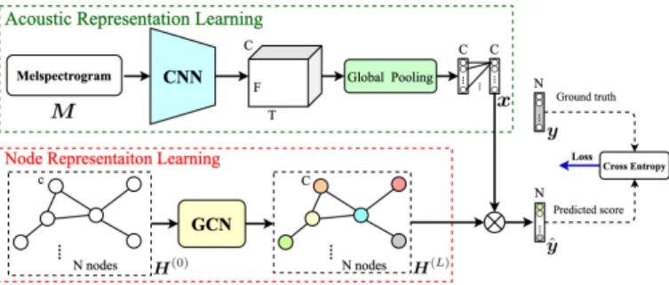
Fig. 1. Overall architecture of our AT-GCN model. Node representations are initially obtained by the word embeddings of the labels and the final node representations learned by GCN are applied to the acoustic representations for classification.
previous layer as inputs and outputs updated node repre-sentations H(l+1) ∈ Rn×c0, where c and c0 indicate the
dimensions of node features in thel-th layer and the(l+ 1)-th layer, respectively. A multi-layer GCN follows the layer-wise propagation rule between the nodes [25]:
H(l+1)=h ˜ D− 1 2A˜D˜− 1 2H(l)W(l) (1) Here, D˜− 1 2A˜D˜−12
is the normalized symmetric adjacency matrix. A˜ = A+IN is the adjacency matrix with added
self-connections (IN is the identity matrix) and D˜ is the
diagonal degree matrix, whereD˜ii=PjA˜ij.W(l)∈Rc×c 0
is a trainable weight matrix, and h(·) denotes an activation function.
III. PROPOSEDMETHOD
In this section, we present a graph-based method to model the label dependencies for audio tagging. The graph structure is constructed by the statistical relations between the labels, and GCN is employed to learn node representations on the graph. The generated node representations are then applied to the acoustic representations for classification, as detailed next.
A. GCN for Audio Tagging
The overall architecture of our proposed model (AT-GCN) is shown in Fig. 1, and CNN10 [11] is used as the baseline model in our experiments. See [11] for details about CNN10.
Acoustic representation learning The aim of acoustic rep-resentation learning module is to extract the acoustic feature from the input log mel spectrogram, and our proposed AT-GCN has the same acoustic representation learning module as CNN10 [11]. Specifically, convolutional layers are applied to the spectrogram M ∈ Rt×f, followed by a global pool-ing layer and a fully-connected layer. Followpool-ing [11], both maximum and average operations are used for global pooling. Let fcnn, fgp, ffc be the operations of the convolutional layers, the global pooling layer and the fully-connected layer, respectively. The acoustic feature x∈RC (where C denotes the dimensionality of the acoustic feature) can be obtained by
x=ffc(fgp(fcnn(M;θcnn)) ;θfc) (2) Here,θcnnandθfc denote the model parameters of the convo-lutional layers and the fully-connected layer, respectively.
Fig. 2. An example of the graph to model the label dependencies. Each node represents a label and each edge represents the relationships between two nodes, which is determined by the conditional probabilities. Note that the edges with small values of the probabilities are filtered by a re-weighting scheme and not shown in the figure.
Node representation learning GCN is employed to learn node representations in our method. As in (1), the stacked multiple GCN layers are applied where each GCN layer takes the node representationsH(l)from the previous layer as inputs and outputs new node representationsH(l+1). The input node representations H(0) ∈RN×c of the first GCN layer are the
word embeddings of the labels, whereN denotes the number of labels and c is the dimensionality of the embeddings. For the last layer (assuming that the number of layers is L), the output isH(L)∈RN×C, whereC equals the dimensionality of the acoustic feature. The predicted score yˆ ∈ RN is then obtained by applying the last node representations to the acoustic representations [28].
ˆ
y=σH(L)x (3) where σ(·) is the sigmoid function to restrict yˆ(i) ∈ (0,1). For the given ground truth of the labels within an audio clip
y∈RN (where y(i)={0,1}denotes whether labeliappears or not), the loss Lis calculated using binary cross-entropy:
L=
N X
i=1
y(i)logyˆ(i)+1−y(i)log1−yˆ(i) (4)
B. Construction of the Graph Structure
The graph structure determines the information propaga-tion between nodes, however, there is no pre-defined graph structure in any audio tagging datasets. In our work, an adjacency matrix is constructed via mining the conditional probabilities between labels within the dataset to represent the graph structure information, as shown in Fig. 2.
Firstly, we count the occurrence of label pairs in the training set and get the matrix X ∈ RN×N (where N indicates the
number of labels, and Xij denotes the co-occurring times of
label Li and Lj). Then, the occurrence times of the labels
in the training set are counted and the conditional probability matrix can be calculated by
Pij=Xij/Ti (5) where Ti denotes the occurrence times of label Li in the training set, Pij = P(Lj|Li) means the probability of label
Lj when label Li appears. Note that Pij is not equal to Pji
Pij, if Pij ≥τ
whereAis the re-weighted adjacency matrix.
Another potential problem is over-smoothing, i.e. as the GCN layer deepens, the node features may be over-smoothed and nodes from different clusters may become indistinguish-able [26], [27]. Thus, we adjust the information propagation among nodes in GCN by another re-weighting scheme:
A0ij=
(
pAij/PNj=1
i6=j Aij, if i6=j
1−p, if i=j (7)
whereA0is the re-weighted and normalized adjacency matrix, andpdetermines the weights assigned to a node itself and its neighbors. Whenp→0, the neighboring information tends to be ignored. On the contrary, whenp→1, the information of a node itself will not be considered.
The proposed algorithm is summarized in Algorithm 1.
Algorithm 1 AT-GCN
Input: The log mel spectrogramM; The initial node repre-sentationsH(0);
Output: The predicted scoreyˆ;
1: Calculate the adjacency matrixAusing equation (5)-(7); 2: Extract the acoustic representationxusing equation (2); 3: forl= 0, . . . , L−1do
4: Get the node representations of the next layerH(l+1)
using equation (1); 5: end for
6: Calculate ˆyaccording to equation (3); 7: returnyˆ;
IV. EXPERIMENTS
A large-scale multi-label dataset (Audioset [21]) is used in our experiments to evaluate our method, which is one of the most challenging datasets for audio tagging [1]. Log mel spectrograms are extracted from the audio signals as the input of the networks. The details are as follows.
A. Dataset, Metrics and Preprocessing
Dataset Audioset [21] is a large-scale dataset with over 2 million 10-second audio clips from YouTube videos, with a total of 527 categories. The training set consists of 2,063,839 audio clips including a balanced subset of 22,160 audio clips. The evaluation set consists of 20,371 audio clips. Following [14], both the balanced and unbalanced training sets are used for training, with one part taken as our validation set. The evaluation set is used as the test set in our experiments.
MetricsMean average precision (mAP), mean area under the curve (mAUC) and d-prime are used as our evaluation metrics.
DeepRes (2019) [5] - 0.392 0.971 2.682 CNN10∗(2019) [11] - 0.422 0.970 2.653 AT-GCN (ours) 1-layer 0.428 0.971 2.711 2-layers 0.434 0.974 2.736 3-layers 0.430 0.972 2.715
∗The listed results of Multi-level attention [9], TAL Net [14] and CNN10
[11] are obtained under the same experimental setups as AT-GCN (e.g. using preprocessing and data augmentation). The original Multi-level attention [9] and TAL Net [14] did not use data augmentation.
TABLE II
ACCURACY COMPARISONS ON DIFFERENT CONSTRUCTION METHODS OF THE ADJACENCY MATRIX
Construction Method mAP mAUC d-prime AT-GCN w/ method in [15], [28] 0.431 0.973 2.727
AT-GCN w/ method in [20] 0.429 0.971 2.701 AT-GCN w/o scheme 0.132 0.907 1.872 AT-GCN w/ scheme in (6) 0.267 0.952 2.360 AT-GCN w/ scheme in (7) 0.188 0.932 2.113 AT-GCN w/ scheme in (6) & (7) 0.434 0.974 2.736
These metrics are calculated on individual classes and then averaged across all classes.
PreprocessingLimited by the computation resource, the pre-extracted log mel spectrograms [14] with window size 50ms and hop length25ms are used in our experiments instead of the raw audio signals, which have lower time domain resolution than those used in [11]. The number of Mel bands is set to 64and the size of a log mel spectrogram is 400×64.
B. Implementation Details
AT-GCNThe node representation learning module of our AT-GCN1consists of two GCN layers with output dimensionality of 256 and 512. It was proven that the performance is hardly impacted by the different initial label representations [28], and following [28], the word embeddings of 300-dim GloVe2 [29] are used as the initial label representations in our experiments. The dimensionality of the acoustic representation is set to512 for a fair comparison with CNN10 [11], and the hyperparametersτ in (6) and p in (7) are set to0.3 and0.2 empirically based on the validation set. PReLU [30] with the negative slope of0.2 is used as the activation function in (1).
Training details In the training phase, the Adam [31] is employed as the optimizer with a learning rate of 0.001. Batch size is set to64 and training takes600,000 iterations. Following [11], data augmentation methods mixup [32] and SpecAugment [33] are applied in our experiments to prevent the system from over-fitting and improve the performance.
1https://github.com/WangHelin1997/AT-GCN 2https://github.com/stanfordnlp/GloVe
Fig. 3. Accuracy comparisons of different values ofτ andpfor AT-GCN with two GCN layers (metric: mAP). Note that whenτ= 1.0,D˜−
1 2A˜D˜−12
in (1) becomes the identity matrix. AT-GCN degenerates to a structure almost identical to CNN10, but with an extra fully-connected layer (as a GCN layer degenerates to a fully-connected layer). As a consequence, the mAP result (42.3%) by AT-GCN is slightly different from that of CNN10 (42.2%).
C. Experimental Results and Analysis
Table I demonstrates the performance of our proposed AT-GCN and other state-of-the-art methods on the Audioset. The results indicate that the proposed AT-GCN outperforms all the compared methods, which confirms the effectiveness of modeling the label dependencies. A single layer GCN learns the node representations by aggregating the information of the immediate neighbors guided by the graph structure information. The results show that AT-GCN with one GCN layer achieves a better performance than the baseline model (CNN10) owing to these statistical relations, which is similar to [16]. While in multi-layer GCN, information is propagated from more neighbors, which implicitly models the deep label dependencies and offers more performance gain. However, increasing the number of GCN layers may lead to over-smoothing [34], which may mix the features of too many nodes and make them indistinguishable. It can be observed that AT-GCN with two GCN layers provides a good trade-off in these aspects and achieves the best performance.
In order to analyze the impacts of the formulation of the adjacency matrix, ablation experiments are carried out. As shown in Table II, AT-GCN does not perform well when no re-weighting scheme is applied because of the over-fitting and over-smoothing problems, which are discussed in Section III-B. In [15], [28], a threshold is set to filter the noisy edges and other edges are treated equally, which is achieved by binarizing the adjacency matrix. However, our proposed re-weighting schemes retain the information of the other edges by only re-weighting the noisy edges and obtain better performance. Both the re-weighting schemes in (6) and (7) improve the performance, and a higher performance can be achieved with the combination of them. In addition, we have tested another construction method of the adjacency matrix [20], which utilizes the ontology rather than the statistical relations. Our proposed method achieves better performance, which shows that the label dependencies are more important in the large-scale multi-label dataset (i.e.Audioset).
In addition, we vary the values of the hyperparameters τin (6) and p in (7) to analyze the effects, and show the results in Fig. 3. As the values of τ and p increase, the accuracy is boosted and then drops, which achieves the peek accuracy when τ = 0.3 and p = 0.2. τ is the threshold to filter the
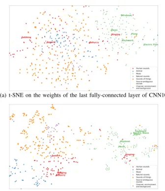
(a) t-SNE on the weights of the last fully-connected layer of CNN10
(b) t-SNE on the last node representations learned by AT-GCN Fig. 4. Visualization of the last node representations learned by AT-GCN and the learned weights of the last fully-connected layer of CNN10 on Audioset. Note that Audioset [21] contains527classes (527 dots in the figure) with
7general categories (the same color dots in the figure). Here,9classes are marked as examples.
edges, and the small values of τ mean the edges of small probabilities (i.e. noisy edges) are filtered. However, when too many edges are filtered, the correlated neighbors will be ignored as well which decreases the accuracy.pdetermines the balance between a node itself and its neighbors when updating the node features. If p is too small, the nodes of the graph cannot get sufficient information from correlated nodes. On the other hand, it will lead to over-smoothing ifpis too large. Furthermore, the t-SNE [36] is adopted to visualize the last node representations (i.e. H(L) in (3)) learned by our proposed AT-GCN as well as the weights of the last fully-connected layer of CNN10, with the results shown in Fig. 4. It can be observed that CNN10 can learn some meaningful relationships among the labels, such as the cluster pattern of the general categorymusic. However, the other cluster patterns are not clear and the semantic related labels (e.g. sobbingand
babycry) are not close in the label space. In contrast, AT-GCN shows less divergence in the label space and exhibits more clear cluster patterns. Specifically, the semantic related labels (such aspianoandkeyboard,sobbingandbabycry) tend to be much closer in the label space than CNN10, which shows the effectiveness of modeling the label dependencies.
V. CONCLUSION
In this paper, a novel audio-tagging method (AT-GCN) has been proposed where the implicit dependencies between the labels are modeled by a graph convolutional network. Our proposed method achieves the state-of-art performance on the Audioset.
[3] Z. Fu, G. Lu, K. M. Ting, and D. Zhang, “A survey of audio-based music classification and annotation,”IEEE Transactions on Multimedia, vol. 13, no. 2, pp. 303–319, 2010.
[4] H. Park and C. D. Yoo, “CNN-Based Learnable Gammatone Filterbank and Equal-Loudness Normalization for Environmental Sound Classifi-cation,”IEEE Signal Processing Letters, 2020.
[5] L. Ford, H. Tang, F. Grondin, and J. Glass, “A Deep Residual Network for Large-Scale Acoustic Scene Analysis,” inProc. Interspeech 2019, 2019, pp. 2568–2572. [Online]. Available: http://dx.doi.org/10.21437/ Interspeech.2019-2731
[6] K. Choi, G. Fazekas, and M. Sandler, “Automatic tagging using deep convolutional neural networks,”arXiv preprint arXiv:1606.00298, 2016. [7] S. Hershey, S. Chaudhuri, D. P. Ellis, J. F. Gemmeke, A. Jansen, R. C. Moore, M. Plakal, D. Platt, R. A. Saurous, B. Seybold et al., “CNN architectures for large-scale audio classification,” in2017 IEEE International Conference on Acoustics, Speech and Signal Processing (ICASSP). IEEE, 2017, pp. 131–135.
[8] E. Cakır, T. Heittola, and T. Virtanen, “Domestic audio tagging with convolutional neural networks,”IEEE AASP Challenge on Detection and Classification of Acoustic Scenes and Events (DCASE 2016), 2016. [9] C. Yu, K. S. Barsim, Q. Kong, and B. Yang, “Multi-level
atten-tion model for weakly supervised audio classificaatten-tion,”arXiv preprint arXiv:1803.02353, 2018.
[10] Q. Kong, C. Yu, Y. Xu, T. Iqbal, W. Wang, and M. D. Plumbley, “Weakly labelled audioset tagging with attention neural networks,”IEEE/ACM Transactions on Audio, Speech, and Language Processing, vol. 27, no. 11, pp. 1791–1802, 2019.
[11] Q. Kong, Y. Cao, T. Iqbal, Y. Wang, W. Wang, and M. D. Plumbley, “PANNs: Large-Scale Pretrained Audio Neural Networks for Audio Pattern Recognition,”arXiv preprint arXiv:1912.10211, 2019. [12] K. Choi, G. Fazekas, M. Sandler, and K. Cho, “Convolutional recurrent
neural networks for music classification,” in2017 IEEE International Conference on Acoustics, Speech and Signal Processing (ICASSP). IEEE, 2017, pp. 2392–2396.
[13] Y. Xu, Q. Kong, W. Wang, and M. D. Plumbley, “Large-scale weakly su-pervised audio classification using gated convolutional neural network,” in2018 IEEE International Conference on Acoustics, Speech and Signal Processing (ICASSP). IEEE, 2018, pp. 121–125.
[14] Y. Wang, J. Li, and F. Metze, “A comparison of five multiple instance learning pooling functions for sound event detection with weak labeling,” in ICASSP 2019-2019 IEEE International Conference on Acoustics, Speech and Signal Processing (ICASSP). IEEE, 2019, pp. 31–35. [15] Y. Sun and S. Ghaffarzadegan, “An ontology-aware framework for
audio event classification,” inICASSP 2020-2020 IEEE International Conference on Acoustics, Speech and Signal Processing (ICASSP). IEEE, 2020, pp. 321–325.
[16] K. Imoto and S. Kyochi, “Sound event detection using graph Lapla-cian regularization based on event co-occurrence,” in ICASSP 2019-2019 IEEE International Conference on Acoustics, Speech and Signal Processing (ICASSP). IEEE, 2019, pp. 1–5.
[17] Y. Xu, Q. Huang, W. Wang, P.J.B. Jackson, and M. D. Plumbley, ”Fully DNN-based multi-label regression for audio tagging”, inWorkshop on Detection and Classification of Acoustic Scenes and Events (DCASE 2016), Budapest, Hungary, 3rd Sept 2016.
[18] M. Cartwright, A. E. M. Mendez, J. Cramer, V. Lostanlen, G. Dove, H.-H. Wu, J. Salamon, O. Nov, and J. P. Bello, “SONYC Urban Sound Tagging (SONYC-UST): a multilabel dataset from an urban acoustic sensor network,” in2019 Workshop on Detection and Classification of Acoustic Scenes and Events (DCASE 2019), 2019, p. 35.
[19] J. P. Bello, C. Silva, O. Nov, R. L. Dubois, A. Arora, J. Salamon, C. Mydlarz, and H. Doraiswamy, “SONYC: A System for Monitoring, Analyzing, and Mtigating Urban Noise Pollution,”Communications of the ACM, vol. 62, no. 2, pp. 68–77, Feb 2019.
[20] H. Shrivaslava, Y. Yin, R. R. Shah, and R. Zimmermann, “MT-GCN for multi-label audio tagging with noisy labels,” inICASSP 2020-2020 IEEE International Conference on Acoustics, Speech and Signal Processing (ICASSP). IEEE, 2020, pp. 136–140.
on Computer Vision and Pattern Recognition, 2016, pp. 2977–2986. [24] C.-W. Lee, W. Fang, C.-K. Yeh, and Y.-C. Frank Wang, “Multi-label
zero-shot learning with structured knowledge graphs,” inProceedings of the IEEE Conference on Computer Vision and Pattern Recognition, 2018, pp. 1576–1585.
[25] T. N. Kipf and M. Welling, “Semi-supervised classification with graph convolutional networks,”arXiv preprint arXiv:1609.02907, 2016. [26] Z. Wu, S. Pan, F. Chen, G. Long, C. Zhang, and P. S. Yu, “A
comprehen-sive survey on graph neural networks,”arXiv preprint arXiv:1901.00596, 2019.
[27] Q. Li, Z. Han, and X.-M. Wu, “Deeper insights into graph convolu-tional networks for semi-supervised learning,” in Thirty-Second AAAI Conference on Artificial Intelligence, 2018.
[28] Z.-M. Chen, X.-S. Wei, P. Wang, and Y. Guo, “Multi-label image recognition with graph convolutional networks,” inProceedings of the IEEE Conference on Computer Vision and Pattern Recognition, 2019, pp. 5177–5186.
[29] J. Pennington, R. Socher, and C. D. Manning, “Glove: Global vectors for word representation,” in Proceedings of the 2014 Conference on Empirical Methods in Natural Language Processing (EMNLP), 2014, pp. 1532–1543.
[30] A. L. Maas, A. Y. Hannun, and A. Y. Ng, “Rectifier nonlinearities improve neural network acoustic models,” inProc. ICML, vol. 30, no. 1, 2013, p. 3.
[31] D. P. Kingma and J. Ba, “Adam: A method for stochastic optimization,” arXiv preprint arXiv:1412.6980, 2014.
[32] H. Zhang, M. Cisse, Y. N. Dauphin, and D. Lopez-Paz, “mixup: Beyond empirical risk minimization,”arXiv preprint arXiv:1710.09412, 2017. [33] D. S. Park, W. Chan, Y. Zhang, C.-C. Chiu, B. Zoph, E. D. Cubuk,
and Q. V. Le, “SpecAugment: A simple data augmentation method for automatic speech recognition,”arXiv preprint arXiv:1904.08779, 2019. [34] G. Li, M. Muller, A. Thabet, and B. Ghanem, “DeepGCNs: Can GCNs Go as Deep as CNNs?” in Proceedings of the IEEE International Conference on Computer Vision, 2019, pp. 9267–9276.
[35] Y. Wang, Y. Sun, Z. Liu, S. E. Sarma, M. M. Bronstein, and J. M. Solomon, “Dynamic graph CNN for learning on point clouds,” Acm Transactions On Graphics (TOG), vol. 38, no. 5, pp. 1–12, 2019. [36] L. V. D. Maaten and G. Hinton, “Visualizing data using t-SNE,”Journal