with Partial Occlusions
Rudolph Triebel1,2and Wolfram Burgard1
1Department of Computer Science, University of Freiburg, Georges-K¨ohler-Allee 79, 79108 Freiburg, Germany
{triebel,burgard}@informatik.uni-freiburg.de
2Autonomous Systems Lab, ETH Zurich, Tannenstraße 3, 8092 Zurich, Switzerland
Summary. In this paper we present an approach to label data points in 3d range scans and to use these labels to learn prototypical representations of objects. Our approach uses associative Markov networks (AMNs) to calculate the labels and a clustering operation to determine the prototypes of homogeneously labeled regions. These prototypes are then used to replace the original regions. In this way, we obtain more accurate models and additionally are able to recover the structure of partially occluded objects. Our approach has been implemented and evaluated on 3d data of a building acquired with a mobile robot. The experimental results demonstrate that our algorithm can robustly identify objects with the same shape and can use the prototypes of these objects for highly accurate mesh completion in case of occlusions.
1 Introduction
Recently, the problem of acquiring three-dimensional models using mobile robots has become quite attractive and a variety of robot systems have been developed that are able to acquire three-dimensional data using laser range scanners [17, 10, 6, 21, 7, 13, 19]. Most of these approaches deal with the problem of how to improve the localization of the robot or how to reduce the huge amount of data by piecewise lin-ear approximations. In this paper we consider the problem of classifying data points in three-dimensional range scans into known classes. The general motivation behind this is to achieve the ability to learn maps that are annotated with symbolic labels. In the past, it has been shown that such information can be utilized to find compact rep-resentations of the maps [19], but also to improve the process of joining partial maps into one big map, usually called map registration by only considering associations between points belonging to corresponding objects [18, 13]. However, a problem arises when these annotated objects are only seen from a partial view or are occluded by other objects. Even if the annotations or labels are correct, corresponding objects can not be found robustly because the entire shape of the objects is not available.
In this paper, we present a supervised learning approach to learn the shape of objects in data points obtained from 3d range scans. Our algorithm applies associa-tive Markov networks (AMNs) [15] to robustly determine segmentations of the data points into different classes. We then perform a clustering operation of the individual segments and calculate a prototype for each segment. In a final step, we replace the individual segments by their prototypes. As a result, we obtain accurate models and even are able to complete partially scanned objects, which frequently appear in the case of occlusions.
The problem of extracting features from range data has been studied intensively in the field of mobile robotics. For example, Buschka and Saffiotti [4] describe a virtual sensor that is able to identify rooms from range data. Additionally, Simmons and Koenig [9] use a pre-programmed routine to detect doorways from range data. Althaus and Christensen [1] use line features to detect corridors and doorways. Also several authors focused on the problem of extracting planar structures from range scans using the expectation maximization algorithm (EM) [10, 12, 19]. Furthermore, there has been work on employing features extracted from three-dimensional range scans to improve the scan alignment process [18, 13]. The approaches described above either operate on two-dimensional scans, consider single features such as pla-narity, or apply pre-programmed routines to identify the features in range scans.
In the context of learning annotated 3D maps from point cloud data several au-thors use the so-called spin images [8, 5] to recognize objects. Vandapel et al. [20] extract saliency features and apply EM to learn a Gaussian Mixture Model classi-fier. Another popular object description technique are shape distributions [14]. In contrast to these approaches, our algorithm classifies the data by also taking into account the potential labels of neighboring data points. This is modeled in a mathe-matical framework known as Markov random fields and improves the segmentation by eliminating false classifications. The recent work by Anguelov et al. [2] applies a similar approach to label data points. However, this technique does not cluster the segments and also cannot complete objects which have been scanned partially only. Fr¨uh and Zakhor [6] generate large-scale 3d-models of urban scenes and apply linear interpolation to deal with partial occlusions. In contrast to this method, our approach extracts object prototypes from range data and uses these prototypes to more accu-rately recover the structure of the scene in the case of occlusions.
This paper is organized as follows. In Section 2, we introduce our scan-point classification technique and an efficient approach to the learning problem. Then, Sec-tion 3 describes our algorithm to handle occlusions in the data sets. Finally, SecSec-tion 4 presents experimental results illustrating the usefulness of our approach.
2 Point Classification using Markov Networks
The first part of our object recognition algorithm consists of a classification for a set of given data points based on a parameter set that was learned from a hand-labeled training data set. For this classification we use an associative Markov network (AMN) [15] which is an instance of a relational Markov network (RMN). RMNs and
AMNs utilize undirected graphical models to represent the conditional probability P(y|x) where y is the set of labels and x the set of features associated to each data point. This is done by defining functions that assign a positive value to each clique in the graph and its associated labeling. These functions are called clique potentials and reflect how well a given labeling fits to a specified clique of graph nodes. In AMNs, the maximum size of a clique is 2, so that only node potentialsϕ(xi,yi) and edge potentialsψ(xi j,yi,yj) exist. Here, we introduce the feature vector xi jof features extracted from the edge between nodes i and j. Likewise, yidenotes the label of node i. Note that the edge feature vector xi jdoes not necessarily have the same size as the node features xi.
Assuming that the network consists of N nodes and a set E = {(i,j)|i,j ∈ {1, . . . ,N},i , j} of edges, the overall conditional probability represented by the AMN can then be formulated as
P(y|x)= 1 Z N Y i=1 ϕ(xi,yi) Y (i j)∈E ψ(xi j,yi,yj). (1)
where Z =Py′QiN=1ϕ(xi,yi′)Q(i j)∈Eψ(xi j,y′i,y′j). Usually, Z is denoted as the parti-tion funcparti-tion and represents the sum of potentials for all possible labelings y′.
It remains to describe the potentialsϕandψ. As mentioned above, the potentials reflect how well the features fit to the labels. One simple way to define the potentials is the log-linear model [15]. In this model, a weight vector wkis introduced for each class label k =1, . . . ,K. The node potentialϕis then defined so that logϕ(xi,yi)= wk
n·xiwhere k=yi. Accordingly, the edge potentials are defined as logψ(xi j,yi,yj)= wke,l·xiwhere k =yiand l = yj. Here we distinguish between weights wn for the nodes and weights wefor the edges. Also, we define the weights depending on the class labels k and l. This means that the potential of node i depends on the label k =yithat is assigned to it. Similarly, the edge potentialψdepends on the labels k and l that are assigned to the nodes connected by the edge. The idea here is that of a relational modeling where the dependencies of the labels are expressed on a higher level, namely the class level. For example, we can model the fact that classes A and B are more strongly related to each other than, say, classes A and C. As a result, the weighting of neighboring points with labels A and B is higher than of points labeled A and C.
To summarize, we define the node and edge potentials as:
ϕ(xi,yi)=exp (wkn·xi) (2) ψ(xi j,yi,yj)=exp (wke,l·xi j) (3)
2.1 Learning and Inference
The scan point segmentation using AMNs is formulated as a supervised learning task. This means that in the learning phase, we are given a set of labels ˆy which were assigned by hand to the training data. Now we learn a set of weights w so that Pw(ˆy|x) is maximized. In the inference phase, these weights are used to find a set
of labels y for the test data set so that Pw(y|x) is maximized. As can be seen from
Equation 1, both steps include the computation of the partition function Z. In all but the simplest cases, the calculation of Z is intractable. For the inference task we can exploit the fact that Z does not depend on the particular labels y. Therefore the maximization of Pw(y|x) is equivalent to maximizing ZPw(y|x). This means that
Z can simply be neglected in the inference step.
However, in the learning task we need to maximize Pw(ˆy|x) over all w, which
means to calculate Z for each w. To overcome this problem, Taskar et al. [16] propose a different way to learn the weights w. Instead of Pw(ˆy|x), they maximize the margin
between the optimal labeling ˆy and any other labeling y defined by
log Pw(ˆy|x)−log Pw(y|x). (4)
This way, the term Zw(x) cancels out and the maximization can be done efficiently.
This method is referred to as maximum margin optimization [16]. The details of this formulation are omitted here for the sake of brevity. We only note that the problem is reduced to a quadratic program (QP) of the form:
min 1 2kwk 2+cξ (5) such that wXˆy+ξ− N X i=1 αi≥N; we≥0; αi− X i j,ji∈E αki j−w k n·xi≥ −ˆy k i ∀i,k; αki j+αkji−wke·xi j≥0 ∀i j∈E,k; αki j, αkji≥0 ∀i j∈E,k
Here, the variables that are solved for in the QP are the weights w=(wn,we), a slack variableξand additional variablesαi,αi j andαji. We refer to Taskar et al. [15] for details.
In the inference task we want to find labels y that maximize log Pw(y | x). As
mentioned above, Z does not depend on y so that the maximization can be done without considering Z. This leads to a linear program of the form
argmax N X i=1 K X k=1 (wkn·xi)yki + X i j∈E K X k=1 (wke·xi j)yki j (6) such that a) yki ≥0, ∀i,k; b) K X k=1 yi=1, ∀i c) yki j≤y k i, y k i j≤y k j, ∀i j∈E,k
Here, we introduced variables yk
i jrepresenting the labels of two points connected by an edge [15].
2.2 Efficient Variant of AMN Learning
Unfortunately, the learning task described in the previous section is computationally expensive with respect to run-time and memory requirements. For each scan point there is one variable and one constraint in the QP. Furthermore, we have two variables and two constraints per edge. This results in a large computational effort (Anguelov et al. [2] report one hour run time for about 30,000 scan points). However, in typi-cal data sets, a huge part of the data is redundant and the data can be substantially reduced by down-sampling. In our experiments we never found evidence that this re-duces the overall performance. The run time dropped from about 20 minutes down to less than a minute while the detection remained at 92%. However, it is not clear how many samples are necessary to obtain good detection rates, because this depends on the data set. A scene with many small objects should not be down-sampled as much as a scene with only few, big objects. Therefore we reduce the data adaptively.
The idea of our adaptive data reduction technique is to obtain as much informa-tion as necessary from the training data so that still a good recogniinforma-tion rate can be achieved. As this depends on the data set, we need an adaptive data structure. One popular way to adaptively store geometrical data are kd-trees. This data structure follows a coarse-to-fine approach: the higher the level in the tree the higher the data abstraction. With kd-trees we can reduce the data set by considering only scan points in the tree that are stored in leaf nodes up to a given maximum depth dmax. All points in deeper branches are then merged into a new leaf node of depth dmax. The data point in this new leaf node is calculated as the mean of all points from the corresponding subtree. Apart from the reduction in the data complexity, this approach makes the sampling less dependent on the data density. The remaining question is how to select dmax. As for the uniform down-sampling, this is dependent on the data set. In our cur-rent system, we therefore modify the reduction algorithm so that it is parameter-free. Instead of pruning at a fixed level, we merge all points in a subtree whenever all of its labels are equal. Accordingly, for large homogeneous areas, where all points have the same label, we obtain a higher level of abstraction than in heterogeneous areas.
3 Occlusion Handling
In most visual recognition tasks we encounter the problem of occlusion: objects are partially hidden by others and therefore can not be recognized robustly. Our approach shows a method to overcome this problem using the semantic knowledge acquired in the learning phase. The idea is to compare objects of the same class to each other and to infer the shape of a single object based on the shapes of the other objects in the class. Hereby we assume that the objects in a class are similar to each other. Based on this assumption, we first group all pointsP={p1, . . . ,pn}that were labeled with the same label in the inference step. Next we cluster all obtained groups according to features defined over the point clouds. Then we match the point clouds for each cluster to each other to obtain the prototypical objects. The meshes calculated for the prototypes are then used to replace the original point clouds.
3.1 Clustering
First, we clusterPinto contiguous subsets which we call entities. The clustering is done using a region-growing algorithm in 3D space where the neighboring relations can be obtained efficiently using a kd-tree. Then, we cluster the entities into sub-classes. The idea here is that usually a class consists of different kinds of objects, e.g., in a class “window” we can find single- and double-size windows as well as windows of different shapes. Of course, the distinction of these subclasses could be done when labeling the training data already. In this case the AMN would automati-cally yield appropriate labels for the individual subclasses. In our current system we decided to separate the division into sub-classes from the labeling process, because it turned out to be difficult to define features for the different entities on the point level. In our implementation we use three entity features based on the oriented bounding box B of the entity and its point cloud P. The features are the volume of B, the quo-tient of the second-longest and the longest edge of B and the radius of P, defined by the maximal distance of a point in P and the centroid of P. Again, for the clustering we apply region-growing, in this case in 3D feature space.
3.2 Entity Matching
In the next step, we match the entities that belong to the same subclass to each other. This is the step in which information about the shape of one entity is used to complete the shape of another entity in the same subclass. This assumes that all entities in a subclass have the same shape and that a good matching between entities can be found. The matching is done using the Iterative Closest Point algorithm (ICP) [3]. In our current implementation, we select one entity as a reference frame and match the other entities to the selected one. One could also think of connecting all entities into a clique and match all entities to each other. Then, the matching errors can be reduced by performing a global optimization of the entity poses. In our experiments, we obtained good results with the one-reference-frame technique. After matching the single entities we obtain a merged point cloud as the prototype of the subclass.
3.3 Mesh Generation
For a better visualization, we generate triangulated meshes from the point cloud re-sulting from the previous step. To this end, we insert all points into a 3D grid. The size of the grid is defined by the oriented bounding box of the point cloud. For each cell c in the grid we store the expected number of points that fall into c, where the probability of falling into c is modeled as an isotropic Gaussian whose mean is the center of c. Then we apply the marching cubes contouring algorithm [11] to find the contour that separates occupied cells from free cells. As a result, we obtain a trian-gular mesh that approximates the volume represented by the point cloud. Finally, we re-project the obtained triangle mesh to all original positions of the singular entities.
4 Experiments
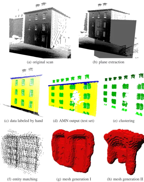
We implemented the described algorithm and tested it on a real data set. The data was collected with a mobile outdoor robot that has a SICK laser range finder and a pan/tilt unit mounted on top for 3D data acquisition. We scanned a building with windows of different kinds and sizes (see 1(a)). In a first step, we divided the data into walls by using a plane extraction algorithm (see Figure 1(b)). Then we extracted all points that had a distance of at most 0.5m from the planes.
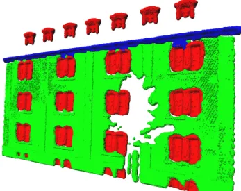
The goal was to classify the scan points into the classes “window”, “wall” and “gutter”. Accordingly, we labeled the training data set manually as shown in Fig-ure 1(c). It consists of one wall with only single-size windows. The original size of the training data set was 36191 data points, while after adaptive reduction we ob-tained a reduced set of 3944 data points. Figure 1(d) shows the result of the AMN based classification on one of our test sets. In a quantitative evaluation we obtained 93.8% correctly classified labels. As we can see from the figure, there are gaps in the data caused by the occlusions of a tree in front of the building. This results in windows that are only partially seen. Figures 1(d)-1(h) show the remaining steps of our algorithm. After applying the last step, namely the back-projection into the scene we obtain the mesh shown in Figure 2. In the scene, all objects have been replaced by the prototypes of the subclasses in which they fall. Note that this holds for all ob-jects in the scene, including the wall and the gutter. The difference compared to the window class is only that for these classes only one object occurs in the data. This means that the prototype of the class is equal to the object encountered. However, for the partially occluded objects, our algorithm was able to recover the full structure.
5 Conclusion
In this paper we presented an approach to segment three-dimensional range data and to use the resulting segments for augmenting the original data. Our approach uses associative Markov networks to robustly extract regions based on an initial labeling obtained with simple geometric features. To efficiently carry out the learning phase, we use an adaptive technique to prune the kd-tree. We then cluster the segments and calculate a prototype for each segment. These prototypes are then used to replace the original segments. The advantage of this approach is two-fold. First, it allows to increase the accuracy of the individual regions, and second it allows to complete partially seen objects by the prototypes.
Our approach has been implemented and tested on data acquired with an outdoor-robot equipped with a laser range finder mounted on a pan/tilt unit. In complex data sets containing outer walls of buildings, our approach has successfully been applied to the task of finding a segmentation into walls, windows, and gutters even in the case of partial occlusions.
(a) original scan (b) plane extraction
(c) data labeled by hand (d) AMN output (test set) (e) clustering
(f) entity matching (g) mesh generation I (h) mesh generation II Fig. 1. The individual steps of our occlusion handling algorithm. From top left to bottom right: a) original 3D scan (no occlusions) b) plane extraction (only one plane is shown), c) hand-labeling of the training data, d) hand-labeling of a test data set obtained with the AMN approach; note that some windows and the wall are occluded, e) class-wise sub-clustering, here for the window class, f) scan matching of all subclusters, here the big windows, g) mesh generation from prototype shown in f), h) mesh for the roof windows prototype.
Fig. 2. Result obtained with our algorithm. Note that two windows in the second column have been restored. In the original data (see Figure 1(d)) these windows were occluded by a tree. Also note that the wall could not be restored, because only one wall object was encountered in the data set so that no prototype containing data in the occluded areas was obtained.
Acknowledgements
This work has partly been supported by the German Research Foundation (DFG) within the Research Training Group 1103 and under contract number SFB/TR-8.
References
1. P. Althaus and H.I. Christensen. Behaviour coordination in structured environments.
Ad-vanced Robotics, 17(7):657–674, 2003.
2. D. Anguelov, B. Taskar, V. Chatalbashev, D. Koller, D. Gupta, G. Heitz, and A. Ng. Dis-criminative Learning of Markov Random Fields for Segmentation of 3D Range Data. In
Conference on Computer Vision and Pattern Recognition (CVPR), 2005.
3. P.J. Besl and N.D. McKay. A method for registration of 3-d shapes. IEEE Transactions
on Pattern Analysis and Machine Intelligence, 14:239–256, 1992.
4. P. Buschka and A. Saffiotti. A virtual sensor for room detection. In Proc. of Intern.
Conference on Intelligent Robots and Systems (IROS), 2002.
5. A. Frome, D. Huber, R. Kolluri, T. Bulow, and J. Malik. Recognizing objects in range data using regional point descriptors. In Proceedings of the European Conference on
Computer Vision (ECCV), 2004.
6. C. Fr¨uh and A. Zakhor. 3d model generation for cities using aerial photographs and ground level laser scans. In Computer Vision and Pattern Recognition Conference, 2001. 7. A. Georgiev and P.K. Allen. Localization methods for a mobile robot in urban
8. A. Johnson and M. Hebert. Using spin images for efficient object recognition in cluttered 3d scenes. IEEE Transactions on Pattern Analysis and Machine Intelligence, 21(5):433– 449, 1999.
9. S. Koenig and R. Simmons. Xavier: A robot navigation architecture based on partially ob-servable markov decision process models. In D. Kortenkamp, R.P. Bonasso, and R. Mur-phy, editors, Artificial Intelligence and Mobile Robots. MIT Press, 1998.
10. Y. Liu, R. Emery, D. Chakrabarti, W. Burgard, and S. Thrun. Using EM to learn 3D models with mobile robots. In Proceedings of the International Conference on Machine
Learning (ICML), 2001.
11. W. E. Lorensen and H. E. Cline. Marching cubes: A high resolution 3D surface construc-tion algorithm. Computer Graphics (SIGGRAPH), 21(4):163–169, 1987.
12. C. Martin and S. Thrun. Online acquisition of compact volumetric maps with mobile robots. In IEEE International Conference on Robotics and Automation (ICRA), Washing-ton, DC, 2002. ICRA.
13. A. N¨uchter, O. Wulf, K. Lingemann, J. Hertzberg, B. Wagner, and H. Surmann. 3d map-ping with semantic knowledge. In RoboCup International Symposium, 2005.
14. R. Osada, T. Funkhouser, B. Chazelle, and D. Dobkin. Matching 3d models with shape distributions. In Shape Modeling International, Genova, Italy, 2001.
15. B. Taskar, V. Chatalbashev, and D. Koller. Learning Associative Markov Networks. In
Twenty First International Conference on Machine Learning, 2004.
16. B. Taskar, C. Guestrin, and D. Koller. Max-Margin Markov Networks. In Neural
Infor-mation Processing Systems Conference, 2003.
17. S. Thrun, W. Burgard, and D. Fox. A real-time algorithm for mobile robot mapping with applications to multi-robot and 3D mapping. In Proc. of the IEEE International
Conference on Robotics&Automation (ICRA), 2000.
18. R. Triebel and W. Burgard. Improving simultaneous localization and mapping in 3d using global constraints. In Proc. of the Twentieth National Conference on Artificial Intelligence
(AAAI), 2005.
19. R. Triebel and W. Burgard. Using hierarchical EM to extract planes from 3d range scans. In Proc. of the IEEE International Conference on Robotics&Automation (ICRA), 2005.
20. N. Vandapel, D. Huber, A. Kapuria, and M. Hebert. Natural terrain classification using 3-d ladar data. In IEEE International Conference on Robotics and Automation, 2004. 21. O. Wulf, K. Arras, H. Christensen, and B. Wagner. 2d mapping of cluttered indoor
envi-ronments by means of 3d perception. In Proc. of the IEEE International Conference on